跳到论文正文
W Papers独立论文阅读器 arXiv:1910.03763 论文正文 计算阅读时间 · 0%
引用这篇论文根据当前论文元数据生成,正式投稿前建议核对。


License: arXiv.org perpetual non-exclusive license
arXiv:1910.03763v2 [gr-qc] 23 Dec 2019

Effective Dynamics from Coherent State Path Integral of Full Loop Quantum Gravity

Muxin Han Affiliation: Department of Physics, Florida Atlantic University, 777 Glades Road, Boca Raton, FL 33431-0991, USA Affiliation: Institut für Quantengravitation, Universität Erlangen-Nürnberg, Staudtstr. 7/B2, 91058 Erlangen, Germany Email: hanm(At)fau.edu    Hongguang Liu Affiliation: Aix Marseille Univ, Universite de Toulon, CNRS, CPT, Marseille, France Affiliation: Laboratoire de Mathématiques et Physique Théorique (UMR CNRS 7350), Université Francois Rabelais, Parc de Grandmont, 37200 Tours, France Affiliation: Laboratoire Astroparticule et Cosmologie, Université Denis Diderot Paris 7, 75013 Paris, France Email: liu.hongguang(At)cpt.univ-mrs.fr
Abstract

A new routine is proposed to relate Loop Quant Cosmology (LQC) to Loop Quantum Gravity (LQG) from the perspective of effective dynamics. We derive the big-bang singularity resolution and big bounce from the first principle of full canonical LQG. Our results are obtained in the framework of the reduced phase space quantization of LQG. As a key step in our work, we derive with coherent states a new discrete path integral formula of the transition amplitude generated by the physical Hamiltonian. The semiclassical approximation of the path integral formula gives an interesting set of effective equations of motion (EOMs) for full LQG. When solving the EOMs with homogeneous and isotropic ansatz, we reproduce the LQC effective dynamics in μ0\mu_{0}-scheme. The solution replaces the big-bang singularity by a big bounce. In the end, we comment on the possible relation between the μ¯\bar{\mu}-scheme of effective dynamics and the continuum limit of the path integral formula.

1 Introduction

Loop Quantum Gravity (LQG) is a promising attempt toward a non-perturbative and background independent theory of quantum gravity (see e.g. book; review; review1 for reviews). Among many important achievements of LQG, one of the most profound physical predictions is the resolution of singularities by quantum effects e.g. Bojowald:2001xe; Ashtekar:2006wn; Ashtekar:2006rx; Singh:2009mz; Assanioussi:2019iye; Ashtekar:2018cay; Ashtekar:2018lag; Assanioussi:2019twp; Gambini:2013hna; BenAchour:2018khr; Bojowald:2018xxu; Bodendorfer:2019cyv; Rovelli:2014cta; Han:2016fgh. It is well-known that the classical theory of Einstein gravity breaks down at singularities, while the purpose of quantum gravity is to extend the gravity theory to describe the physics of singularities.

The first concrete example of resolving singularity in LQG was made in Loop Quantum Cosmology (LQC) Bojowald:2001xe; Ashtekar:2006wn; Ashtekar:2006rx (see e.g. Bojowald:2006da; Ashtekar:2008zu; Agullo:2016tjh for reviews on LQC). LQC applies the quantization procedure of LQG to the homogeneous and isotropic sector of gravity. The classical symmetry-reduction to the homogeneous and isotropic sector reduces from infinitely many degrees of freedom (DOFs) of gravity to a single DOF (the scale factor). Then LQC quantizes the 2-dimensional phase space of cosmology by LQG method and imposes Hamiltonian constraint at the quantum level. The quantum dynamics of LQC have been studied extensively. It has been shown that the quantum evolution of coherent state in LQC gives rise to an effective equation, which reduces to classical Friedmann equation at low energy density regiem, while modifying Friedmann equation at high energy density near the big-bang singularity Taveras:2008ke. The solution of effective equation demonstrates that the big-bang singularity is resolved and replaced by a big bounce, where the curvature is finite and Planckian. The time evolution of cosmology governed by the LQC effective equation is often called the effective dynamics.

However LQC, from quantization after classical symmetry-reduction, only takes into account DOFs that are homogeneous and isotropic, thus fails to predict for instance quantum fluctuations beyond the homogeneous and isotropic sector Bojowald:2018sgf. Moreover LQC has been suffered from the long-standing issue on the relation with the full theory of LQG (see e.g. Alesci:2013xd; Bodendorfer:2014vea; Bodendorfer:2015hwl; Alesci:2016rmn; Dapor:2017rwv; Engle:2007zz; 2016arXiv160105531H; Fleischhack:2010zt; Rovelli:2008aa for some earlier works on this perspective). It has not been clarified if the singularity resolution and big bounce can be derived from the first principle of full LQG. Symmetry-reduced models of loop quantum black holes share the same issues as LQC.

Our present work partially addresses the above issues of LQC. We propose a new routine to relate LQC to LQG from the perspective of effective dynamics, and demonstrate the singularity resolution and big bounce from the first principle of the full canonical LQG. Our results are obtained in the framework of the reduced phase space quantization of LQG. As a key step in our work, we derive with coherent states a new discrete path integral formula of the transition amplitude generated by the physical Hamiltonian. The semiclassical approximation of the path integral formula gives an interesting set of effective equations of motion (EOMs) of full LQG. When solving the EOMs with homogeneous and isotropic ansatz, we reproduce the solution of LQC effective dynamics in μ0\mu_{0}-scheme. The solution replaces the big-bang singularity by a big bounce.

Since our framework embeds the cosmological effective dynamics in the path integral formulation of full LQG, all quantum fluctuations within and beyond the homogenous and isotropic sector are in principle computable by e.g. perturbative expansion or other non-perturbative methods.

Our work takes advantage of the reduced phase space quantization of LQG Giesel:2007wn; Giesel:2012rb and studies the quantum dynamics given by the full LQG physical Hamiltonian 𝐇^\hat{\bf H} defined on the physical Hilbert space ℋ\mathcal{H} of Dirac observables. The reduced phase space quantization is based on classical deparametrized models of gravity such as gravity coupled to dust fields or scalars. Our work takes into account three different scenarios: gravity coupled to the Brown-Kuchař dust, gaussian dust, and massless scalar field Brown:1994py; Kuchar:1990vy; Giesel:2007wn; Giesel:2012rb; Domagala:2010bm; Rovelli:1993bm. In the quantum theory, we set the Hilbert space ℋ=ℋγ\mathcal{H}=\mathcal{H}_{\gamma} to be based on a fixed graph γ\gamma which is a finite cubic lattice partitioning 3-torus 11 1 The result is also valid in the case of an infinite space., and define 𝐇^\hat{\bf H} to be the non-graph-changing Hamiltonian.

There are two popular Hamiltonians of LQG, based on Giesel-Thiemann’s construction QSD; Giesel:2007wn, and the construction by Alesci-Assanioussi-Lewandowski-Makinen (AALM) Alesci:2015wla; Assanioussi:2015gka using scalar curvature operator Alesci:2014aza. Our work analyzes both possibilities.

The seminal works Thiemann:2000bw; Thiemann:2000ca; Thiemann:2000bx tell us that the Hilbert space ℋ\mathcal{H} has an over-complete basis given by the complexifier coherent states ψgt\psi^{t}_{g}, where at each edge e∈E⁡(γ)e\in E(\gamma)22 2 E⁡(γ)E(\gamma) and V⁡(γ)V(\gamma) denote the set of edges and vertices in γ\gamma., the coherent state label g={g⁡(e)}e∈E⁡(γ)g=\{g(e)\}_{e\in E(\gamma)} with g(e)=e−ipa(e)τa/2h(e)=e−ipa(e)τa/2eθa​(e)​τa/2∈SL(2,ℂ)g(e)=e^{-ip^{a}(e)\tau^{a}/2}h(e)=e^{-ip^{a}(e)\tau^{a}/2}e^{\theta^{a}(e)\tau^{a}/2}\in\mathrm{SL}(2,\mathbb{C}) is the holomorphic coordinate on the LQG phase space of holonomies h⁡(e)h(e) and gauge covariant fluxes pa​(e)p^{a}(e). The dimensionless semiclassicality parameter t=ℓP2/a2t=\ell_{P}^{2}/a^{2} where ℓP2=ℏ​κ\ell_{P}^{2}=\hbar\kappa is the Planck scale, and aa is a length unit e.g. 1cm. The semiclassical limit is given by t→0t\to 0 or ℓP≪a\ell_{P}\ll a. Thanks to the overcompleteness and semiclassical properties of coherent states, and by the standard discretization and coherent state path integral method, the transition amplitude between gauge invariant coherent states ⟨Ψ[g]t|exp⁡[−iℏ​𝐇^​T]|Ψ[g′]t⟩\langle\Psi^{t}_{[g]}|\,\exp[-\frac{i}{\hbar}\hat{\bf H}T]\,|\Psi^{t}_{[g^{\prime}]}\rangle can be written as a discrete path integral formula (see Section 3 for details)

∫d​h​∏i=1N+1d​gi​ν​[g]​eS⁡[g,h]/t,\displaystyle\int\mathrm{d}h\prod_{i=1}^{N+1}\mathrm{d}g_{i}\,\nu[g]\,e^{S[{g},h]/t}, (1)

where the integral is over N+1N+1 intermediate states gi∈SL​(2,ℂ)|E⁡(γ)|g_{i}\in\mathrm{SL}(2,\mathbb{C})^{|E(\gamma)|} and h={hv}v∈V⁡(γ)∈SU​(2)|V⁡(γ)|h=\{h_{v}\}_{v\in V(\gamma)}\in\mathrm{SU}(2)^{|V(\gamma)|} (for ensuring SU(2) gauge invariance). ν⁡[g]\nu[g] is a path integral measure. S⁡[g,h]S[{g},h] is the effective action for LQG extracted from the path integral:

S⁡[g,h]\displaystyle S[g,h] =\displaystyle= ∑i=0N+1K⁡(gi+1,gi)−i​κa2​∑i=1NΔ​τ​⟨ψgi+1t|𝐇^|ψgit⟩⟨ψgi+1t|ψgit⟩\displaystyle\sum_{i=0}^{N+1}K\left(g_{i+1},g_{i}\right)-\frac{i\kappa}{a^{2}}\sum_{i=1}^{N}\Delta\tau\frac{\left\langle\psi_{g_{i+1}}^{t}|\hat{\mathbf{H}}|\psi_{g_{i}}^{t}\right\rangle}{\left\langle\psi_{g_{i+1}}^{t}|\psi_{g_{i}}^{t}\right\rangle} (2)
K⁡(gi+1,gi)\displaystyle K\left(g_{i+1},g_{i}\right) =\displaystyle= ∑e∈E⁡(γ)[zi+1,i​(e)2−12​pi+1​(e)2−12​pi​(e)2]\displaystyle\sum_{e\in E(\gamma)}\left[z_{i+1,i}(e)^{2}-\frac{1}{2}p_{i+1}(e)^{2}-\frac{1}{2}p_{i}(e)^{2}\right] (3)

The discretization step Δ​τ=T/N\Delta\tau=T/N is arbitrarily small while NN is arbitrarily large. Here zi+1,i​(e)z_{i+1,i}(e) relates to gi​(e),gi+1​(e)g_{i}(e),g_{i+1}(e) by zi+1,i​(e)=arccosh⁡(12​tr​[gi+1​(e)†​gi​(e)])z_{i+1,i}(e)=\mathrm{arccosh}(\frac{1}{2}\mathrm{tr}[g_{i+1}(e)^{\dagger}g_{i}(e)]). S⁡[g,h]S[g,h] depends on hh through g0=g′h=hs⁡(e)−1​{g′​(e)​ht⁡(e)}e∈E⁡(γ)g_{0}=g^{\prime h}=h_{s(e)}^{-1}\{g^{\prime}(e)h_{t(e)}\}_{e\in E(\gamma)} where g′g^{\prime} is the initial data. gN+2=gg_{N+2}=g is the final data.

To our knowledge, this path integral formula Eq.1 of the full LQG hasn’t been derived before, although it has been motivated in e.g. link; Han:2009bb. It should shed light on the relation between canonical LQG and Spinfoam formulation. Interestingly in the scenario of gravity coupled to scalar field and AALM Hamiltonian, this path integral formula should be the coherent state representation of the spinfoam model in Kisielowski:2018oiv if their model was defined with a non-graph-changing Hamiltonian.

The path integral formula in the context of LQC is studied in Ashtekar:2009dn; Henderson:2010qd; Craig:2016iuw; Craig:2016lxm. The coherent state path integral is applied to LQC in Qin:2012xh.

The discrete path integral Eq.1 is well-defined as a finite integral as far as NN is finite (although arbitrarily large). The semiclassical limit t→0t\to 0 motivates us to apply the stationary phase approximation. The integral is dominated by contributions from solutions of the EOM obtained from the variational principle δ​S​[g,h]=0\delta S[g,h]=0. We propose that the cosmological effective dynamics should emerge from solutions of EOM given by the path integral of full LQG. Here the EOM may be (aa) the classical EOM obtained from the stationary phase approximation, or (bb) the quantum EOM derived from the quantum effective action which includes all quantum corrections. Our work focuses on the proposal (a)(a).

The EOMs from the semiclassical approximation of the path integral Eq.1 is derived in Section 4: In the continuous time approximation Δ​τ→0\Delta\tau\to 0, we obtain

  • •

    For i=1,⋯,Ni=1,\cdots,N, at every edge e∈E⁡(γ)e\in E(\gamma),

    zi+1,i​(e)​tr​[τa​gi+1​(e)†​gi​(e)]xi+1,i​(e)−1​xi+1,i​(e)+1−pi​(e)​tr​[τa​gi​(e)†​gi​(e)]sinh⁡(pi​(e))=i​κ​Δ​τa2​∂𝐇⁡[giε]∂εa​(e)|ε→=0\displaystyle\frac{z_{i+1,i}(e)\,\mathrm{tr}\left[\tau^{a}g_{i+1}(e)^{\dagger}g_{i}(e)\right]}{\sqrt{x_{i+1,i}(e)-1}\sqrt{x_{i+1,i}(e)+1}}-\frac{p_{i}(e)\,\mathrm{tr}\left[\tau^{a}g_{i}(e)^{\dagger}g_{i}(e)\right]}{\sinh(p_{i}(e))}=\frac{i\kappa\Delta\tau}{a^{2}}\frac{\partial\,{\mathbf{H}\left[g_{i}^{\varepsilon}\right]}}{\partial{\varepsilon^{a}(e)}}\Bigg|_{\vec{\varepsilon}=0} (4)
  • •

    For i=2,⋯,N+1i=2,\cdots,N+1, at every edge e∈E⁡(γ)e\in E(\gamma),

    zi,i−1​(e)​tr​[τa​gi​(e)†​gi−1​(e)]xi,i−1​(e)−1​xi,i−1​(e)+1−pi​(e)​tr​[τa​gi​(e)†​gi​(e)]sinh⁡(pi​(e))=−i​κ​Δ​τa2​∂𝐇⁡[giε]∂ε¯a​(e)|ε→=0.\displaystyle\frac{z_{i,i-1}(e)\,\mathrm{tr}\left[\tau^{a}g_{i}(e)^{\dagger}g_{i-1}(e)\right]}{\sqrt{x_{i,i-1}(e)-1}\sqrt{x_{i,i-1}(e)+1}}-\frac{p_{i}(e)\,\mathrm{tr}\left[\tau^{a}g_{i}(e)^{\dagger}g_{i}(e)\right]}{\sinh(p_{i}(e))}=-\frac{i\kappa\Delta\tau}{a^{2}}\frac{\partial\,{\mathbf{H}\left[g_{i}^{\varepsilon}\right]}}{\partial{\bar{\varepsilon}^{a}(e)}}\Bigg|_{\vec{\varepsilon}=0}. (5)
  • •

    The closure condition at every vertex v∈V⁡(γ)v\in V(\gamma) for initial data:

    −∑e,s⁡(e)=vp1a(e)+∑e,t⁡(e)=vΛba(θ→1(e))p1b(e)=0.\displaystyle-\sum_{e,s(e)=v}p_{1}^{a}(e)+\sum_{e,t(e)=v}\Lambda^{a}_{\ b}\left(\vec{\theta}_{1}(e)\right)\,p_{1}^{b}(e)=0. (6)

In the above, zi+1,i​(e)z_{i+1,i}(e) and xi+1,i​(e)x_{i+1,i}(e) are given by zi+1,i​(e)=arccosh⁡(xi+1,i​(e))z_{i+1,i}(e)=\mathrm{arccosh}\left(x_{i+1,i}(e)\right), xi+1,i​(e)=12​tr​[gi+1​(e)†​gi​(e)]x_{i+1,i}(e)=\frac{1}{2}\mathrm{tr}\left[g_{i+1}(e)^{\dagger}g_{i}(e)\right]. The initial and final conditions are given by g1=g′hg_{1}=g^{\prime}{}^{h} and gN+1=gg_{N+1}=g. 𝐇⁡[gε]{\bf H}[g^{\varepsilon}] is the classical physical Hamiltonian discretized on the lattice γ\gamma, and evaluated at the phase space point gε​(e)=g⁡(e)​eεa​(e)​τag^{\varepsilon}(e)=g(e)e^{\varepsilon^{a}(e)\tau^{a}}. Λba​(θ→)∈SO⁡(3)\Lambda^{a}_{\ b}(\vec{\theta})\in\mathrm{SO(3)} is given by eθa​τa/2τae−θaτa/2=Λba(θ→)τbe^{\theta^{a}\tau^{a}/2}\tau^{a}e^{-\theta^{a}\tau^{a}/2}=\Lambda^{a}_{\ b}(\vec{\theta})\tau^{b}.

We may call Eqs.4, 5, and 6 effective equations if we call S⁡[g,h]S[g,h] the effective action. These effective equations are interesting because

  • •

    They govern the semiclassical dynamics of full LQG, and are valid for all dynamical scenarios/spacetimes.

  • •

    All ingredients of the equations are explicitly computable. The equations are solvable analytically or numerically. In particular, Eqs.4 and 5 are dynamical evolution equations with natural discretization implied by LQG. They are ready for numerically simulation and can relate to numerical relativity.

  • •

    Quantum correction can be computed (by perturbative expansion or other non-perturbative methods) since these equations are derived from path integral formula. In contrast of the LQC effective dynamics, we can take into account all quantum fluctuations in our framework.

In Sections 5 and 6, we apply the above effective EOMs to cosmology. To search for the cosmological solution, we insert the following ansatz respecting the homogeneous and isotropic symmetries

gi​(eI​(v))=e(θi−i​pi)​τI2,\displaystyle g_{i}(e_{I}(v))=e^{\left(\theta_{i}-{i}p_{i}\right)\frac{\tau^{I}}{2}}, (7)

where θi\theta_{i} and pip_{i} are constants on every spatial slice, and relates to holonomies and fluxes by

hi​(eI​(v))≡hi​(I)=eθi​τI/2pia​(eI​(v))≡pia​(I)=pi​δIa.\displaystyle h_{i}(e_{I}(v))\equiv h_{i}(I)=e^{\theta_{i}\tau_{I}/2}\quad p^{a}_{i}(e_{I}(v))\equiv p_{i}^{a}(I)=p_{i}\,\delta^{a}_{I}. (8)

EOMs 4, 5, and 6 are simplified by the above ansatz, and interestingly reproduces the LQC effective equations in μ0\mu_{0}-scheme. The solution resolves big-bang singularity in all scenarios of gravity coupled to the Brown-Kuchař dust, Gaussian dust, and massless scalar. The big-bang singularity is replaced by an (time-refection) unsymmetric bounce in the case of the Giesel-Thiemann’s Hamiltonian. The bounce is symmetric in the case of Alesci-Assanioussi-Lewandowski-Makinen’s Hamiltonian.

The above summarizes our strategy to derive the cosmological effective dynamics and singularity resolution in full LQG from top to down. We would like to mention that our work is inspired by the work by Dapor and Liegener Dapor:2017rwv where they propose the LQC effective dynamics to be generated by the cosmological coherent state expectation value of H^\hat{H} of full LQG, and demonstrate the unsymmetric bounce (their effective equation coincides with the one proposed earlier by Ding, Ma, and Yang in Yang:2009fp). However in their scheme, the relation with the full LQG relies on the conjecture of existing dynamically stabled coherent state. But this conjecture is difficult to verify. It is usually difficult to find dynamically stable coherent state in interacting quantum field theories. However lessons from quantum field theory indicate that path integral should be the most powerful tool for studying effective theories. Our work suggests to use path integral for deriving effective dynamics in LQG and bypassing the difficulty of finding dynamically stable coherent state.

In Section 8, we compute the contribution of the cosmological solutions to the transition amplitude in the semiclassical approximation, and show that in a formal continuum limit of the lattice γ\gamma, the contribution is independent of the choice of Hamiltonian.

The cosmological effective dynamics obtained here correspond to the μ0\mu_{0}-scheme of LQC. It is known that in LQC, the μ0\mu_{0}-scheme suffers the problem that the bounce may happen at low critical density (or large critical volume), and the better scheme is the μ¯\bar{\mu}-scheme where the critical density is Plankian (see e.g. Ashtekar:2006wn; Assanioussi:2019iye). In Section 9, we comment on the problem of μ0\mu_{0}-scheme from the full LQG point of view, and suggest that if we take into account of the continuum limit of the lattice γ\gamma, the critical density should be always high in our framework. However the continuum limit requires to take non-perturbative quantum corrections into consideration, and is beyond the scope of this paper (see some recent work e.g. Dittrich:2014ala; Bahr:2016hwc; Lang:2017beo; Han:2018fmu on the continuum limit in LQG). We propose that the μ¯\bar{\mu}-scheme should relate to the quantum effective EOM, which may be derived from the quantum effective action of our path integral.

The architecture of this paper is the following: Firstly in Section 2 we review briefly some key results and tools in the reduced phase space quantization of LQG and complexifier coherent states. Section 3 derives the path integral formula from the transition amplitude of full LQG. Section 4 derives the effective EOMs of full LQG from the variational principle. Section 5 studies the effective EOMs with the homogeneous and isotropic ansatz. Section 6 derives the cosmological effective equations with different choices of Hamiltonians. Section 7 obtains the solution with singularity resolution and unsymmetric/symmetric bounce. Section 8 computes the on-shell action and the semiclassical approximation of the transition amplitude. Section 9 discusses the relation between the continuum limit and effective dynamics in μ¯\bar{\mu}-scheme, as well as a few other future perspectives.

2 Preliminaries

2.1 Reduced phase space quantization of LQG

Several models have been proposed to introduce scalar material reference frame and deparametrize GR into systems with physical Hamiltonians (see e.g. Kuchar:1990vy; Brown:1994py; Giesel:2007wn; Alesci:2015wla; Giesel:2012rb; Husain:2011tk). The deparametrization procedure solves Hamiltonian and diffeomorphism constraints classically and construct models in terms of Dirac observables. These models have physical time evolution generated by physical Hamiltonian. LQG quantization of these models bypass the standard difficulty of solving quantum Hamiltonian constraint, because Hilbert spaces and operators are resulting from quantizing Dirac observables.

Among models of deparametrized GR, our analysis takes into account 3 different scenarios: the Brown-Kuchař dust, Gaussian dust, and massless scalar field: Firstly, we denote by SB​K​DS_{BKD} and SG​DS_{GD} the dust actions of Brown-Kuchař and Gaussian dust models Brown:1994py; Kuchar:1990vy; Giesel:2007wn; Giesel:2012rb:

SB​K​D​[ρ,gμ​ν,T,Sj,Wj]\displaystyle S_{BKD}[\rho,g_{\mu\nu},T,S^{j},W_{j}] =\displaystyle= −12∫d4x|det(g)|ρ[gμ​νUμUν+1],Uμ=−∂μT+Wj∂μSj,\displaystyle-\frac{1}{2}\int\mathrm{d}^{4}x\ \sqrt{|\det(g)|}\ \rho\ [g^{\mu\nu}U_{\mu}U_{\nu}+1],\quad U_{\mu}=-\partial_{\mu}T+W_{j}\partial_{\mu}S^{j}, (9)
SG​D​[ρ,gμ​ν,T,Sj,Wj]\displaystyle S_{GD}[\rho,g_{\mu\nu},T,S^{j},W_{j}] =\displaystyle= −∫d4x|det(g)|[ρ2(gμ​ν∂μT∂νT+1)+gμ​ν∂μT(Wj∂νSj)],\displaystyle-\int\mathrm{d}^{4}x\ \sqrt{|\det(g)|}\left[\frac{\rho}{2}\ \left(g^{\mu\nu}\partial_{\mu}T\partial_{\nu}T+1\right)+g^{\mu\nu}\partial_{\mu}T\left(W_{j}\partial_{\nu}S^{j}\right)\right], (10)

where T,Sj=1,2,3T,S^{j=1,2,3} form the dust reference frame, and ρ,Wj\rho,\ W_{j} are Lagrangian multipliers. When we couple either SB​K​DS_{BKD} or SG​DS_{GD} to Einstein gravity and carry out the Hamiltonian analysis Giesel:2012rb, the total Hamiltonian and diffeomorphism constraints can be cast in the following form (α=1,2,3\alpha=1,2,3)

Ct​o​t\displaystyle C^{tot} =\displaystyle= P+h⁡(p,q,∂αT),\displaystyle P+h(p,q,\partial_{\alpha}T), (11)
Cjt​o​t\displaystyle C^{tot}_{j} =\displaystyle= Pj+Sjα​[Cα​(p,q)+P​∂αT],\displaystyle P_{j}+S^{\alpha}_{j}\left[C_{\alpha}(p,q)+P\partial_{\alpha}T\right], (12)

which are strongly Poisson commutative. SjαS^{\alpha}_{j} is the inverse matrix of ∂αSj\partial_{\alpha}S^{j} (α=1,2,3\alpha=1,2,3), P,PjP,P_{j} are momenta conjugate to T,SjT,S^{j}, and p,qp,q denote canonical variables of gravity. CαC_{\alpha} are the diffeomorphism constraint of gravity. The classical constraints Ct​o​t=Cjt​o​t=0C^{tot}=C^{tot}_{j}=0 are solved by P=−hP=-h and Pj=−Sjα​[Cα​(p,q)+P​∂αT]P_{j}=-S^{\alpha}_{j}\left[C_{\alpha}(p,q)+P\partial_{\alpha}T\right]. Gauge invariant Dirac observables are constructed relationally by parametrizing gravity variables with values of dust fields T⁡(x)≡τ,Sj​(x)≡σjT(x)\equiv\tau,S^{j}(x)\equiv\sigma^{j}, e.g. p⁡(σ,τ)=p⁡(x)|T⁡(x)≡τ,Sj​(x)≡σjp(\sigma,\tau)=p(x)|_{T(x)\equiv\tau,\,S^{j}(x)\equiv\sigma^{j}} and q⁡(σ,τ)=q⁡(x)|T⁡(x)≡τ,Sj​(x)≡σjq(\sigma,\tau)=q(x)|_{T(x)\equiv\tau,\,S^{j}(x)\equiv\sigma^{j}}, where σ,τ\sigma,\tau are physical space and time coordinates in the dust frame.

We choose gravity canonical variables as su(2) Ashtekar-Barbero connection Aja​(σ,τ)A_{j}^{a}(\sigma,\tau) and densitized triad Eaj​(σ,τ)E^{j}_{a}(\sigma,\tau). Both Aja​(σ,τ)A_{j}^{a}(\sigma,\tau) and Eaj​(σ,τ)E^{j}_{a}(\sigma,\tau) are Dirac observables (a=1,2,3a=1,2,3 is the su(2) index and j=1,2,3j=1,2,3 is the coordinate index in 𝒮\mathcal{S}). They satisfy the Poisson bracket {Eai​(σ,τ),Ajb​(σ′,τ)}=12​κ​β​δji​δab​δ3​(σ,σ′)\{E^{i}_{a}(\sigma,\tau),A_{j}^{b}(\sigma^{\prime},\tau)\}=\frac{1}{2}\kappa\beta\delta^{i}_{j}\delta^{b}_{a}\delta^{3}(\sigma,\sigma^{\prime}) where β\beta is the Barbero-Immirzi parameter and κ=16​π​G\kappa=16\pi G. The phase space 𝒫\mathcal{P} of Aja​(σ,τ),Eaj​(σ,τ)A_{j}^{a}(\sigma,\tau),E^{j}_{a}(\sigma,\tau) is free of Hamiltonian and diffeomorphism constraints, and all phase space functions are Dirac observables.

As an important Dirac observable, the physical Hamiltonian is given by integrating hh on the constant T=τT=\tau slice 𝒮\mathcal{S}: 𝐇=∫𝒮d3​σ​h|∂αT=0\mathbf{H}=\int_{\mathcal{S}}\mathrm{d}^{3}\sigma\,h|_{\partial_{\alpha}T=0} Giesel:2007wn; Giesel:2012rb,

Brown-Kuchař dust: 𝐇=∫𝒮d3​σ​C​(σ,τ)2−14​∑j=13Cj​(σ,τ)​Cj​(σ,τ),\displaystyle\mathbf{H}=\int_{\mathcal{S}}\mathrm{d}^{3}\sigma\,\sqrt{C(\sigma,\tau)^{2}-\frac{1}{4}\sum_{j=1}^{3}C_{j}(\sigma,\tau)C_{j}(\sigma,\tau)}, (13)
Gaussian dust: 𝐇=∫𝒮d3​σ​C​(σ,τ).\displaystyle\mathbf{H}=\int_{\mathcal{S}}\mathrm{d}^{3}\sigma\,C(\sigma,\tau). (14)

The constant τ\tau slice 𝒮\mathcal{S} is coordinated by the value of dust scalars Sj=σjS^{j}=\sigma^{j} thus is often referred to as the dust space Giesel:2007wn; Giesel:2012rb. The physical Hamiltonian 𝐇\mathbf{H} generates the τ\tau-time evolution:

d​fd​τ={𝐇,f},\displaystyle\frac{\mathrm{d}f}{\mathrm{d}\tau}=\left\{\mathbf{H},f\right\}, (15)

for all phase space function ff of Aja​(σ,τ)A_{j}^{a}(\sigma,\tau) and Eaj​(σ,τ)E^{j}_{a}(\sigma,\tau). In either the Brown-Kuchař or the Gaussian dust model, 𝐇\mathbf{H} relates to the Hamiltonian and diffeomorphism constraints C⁡(σ,τ),Cj​(σ,τ)C(\sigma,\tau),C_{j}(\sigma,\tau) evaluated on 𝒮\mathcal{S}. C⁡(σ,τ),Cj​(σ,τ)C(\sigma,\tau),C_{j}(\sigma,\tau) are in terms of Aja​(σ,τ)A_{j}^{a}(\sigma,\tau) and Eaj​(σ,τ)E^{j}_{a}(\sigma,\tau):

C\displaystyle C =\displaystyle= −2κ​det(q)​tr​(Fj​k​[Ej,Ek])+2​(1−s​β2)κ​det(q)​tr​([Kj,Kk]​[Ej,Ek]),\displaystyle-\frac{2}{\kappa\sqrt{\det(q)}}\mathrm{tr}\left(F_{jk}\left[E^{j},E^{k}\right]\right)+\frac{2({1-s\beta^{2}})}{\kappa\sqrt{\det(q)}}\mathrm{tr}\left(\left[K_{j},K_{k}\right]\left[E^{j},E^{k}\right]\right), (16)
Cj\displaystyle C_{j} =\displaystyle= −2κ​det(q)​tr​(τj​Fk​l​[Ek,El]).\displaystyle-\frac{2}{\kappa\sqrt{\det(q)}}\mathrm{tr}\left(\tau_{j}F_{kl}\left[E^{k},E^{l}\right]\right). (17)

where Ej=Eaj​τa/2E^{j}=E^{j}_{a}\tau^{a}/2, Kj=Kja​τa/2K_{j}=K_{j}^{a}\tau^{a}/2 is the extrinsic curvature, and Fj​k=Fj​ka​τa/2F_{jk}=F_{jk}^{a}\tau^{a}/2 is the curvature of Aj=Aja​τa/2A_{j}=A_{j}^{a}\tau^{a}/2. τa=−i​(Pauli matrix)a\tau^{a}=-i(\text{Pauli matrix})^{a}. s=1s=1 or −1-1 corresponds respectively to the Euclidean or Lorentzian signature.

The gravity-dust models only deparametrize the Hamiltonian and diffeomorphism constraints, while the SU(2) Gauss constraint Dj​Ej=0D_{j}E^{j}=0 still has to be imposed to the classical phase space. In addition, we impose some non-holonomic constraints to the phase space. In the Brown-Kuchař dust model, solving Ct​o​t=Cjt​o​t=0C^{tot}=C^{tot}_{j}=0 restricts C​(σ,τ)2−14​∑j=13Cj​(σ,τ)​Cj​(σ,τ)≥0C(\sigma,\tau)^{2}-\frac{1}{4}\sum_{j=1}^{3}C_{j}(\sigma,\tau)C_{j}(\sigma,\tau)\geq 0. In the Gaussian dust model, we split the phase space 𝒫\mathcal{P} into two sector C⁡(σ,τ)≥0C(\sigma,\tau)\geq 0 and C⁡(σ,τ)<0C(\sigma,\tau)<0, where we can write 𝐇=∫𝒮d3​σ​|C⁡(σ,τ)|\mathbf{H}=\int_{\mathcal{S}}\mathrm{d}^{3}\sigma\,|C(\sigma,\tau)| and 𝐇=−∫𝒮d3σ|C(σ,τ)|\mathbf{H}=-\int_{\mathcal{S}}\mathrm{d}^{3}\sigma\,|C(\sigma,\tau)| respectively. Note that since we consider the dust is the only matter coupling to gravity, we work with physical Brown-Kuchař dust with positive energy density in order to fulfill the energy condition. We also choose the physical time τ\tau to flow backward in order to make 𝐇{\bf H} positive (see Giesel:2007wi for details).

A real massless scalar field coupling to gravity is another interesting deparametrized model for reduced phase space quantization. We minimally couple the following scalar field action to gravity:

Sϕ[gμ​ν,ϕ]=−12∫d4x|det(g)|gμ​ν∂μϕ∂νϕ.\displaystyle S_{\phi}[g_{\mu\nu},\phi]=-\frac{1}{2}\int\mathrm{d}^{4}x\ \sqrt{|\det(g)|}\,g^{\mu\nu}\partial_{\mu}\phi\,\partial_{\nu}\phi. (18)

Similar to TT in the above dust models, the value of the real scalar ϕ⁡(x)=τ\phi(x)=\tau plays the role of the physical time variable. Canonical variables of gravity are parametrized by the physcical time τ\tau: p⁡(x→,τ)=p⁡(x)|ϕ⁡(x)≡τp(\vec{x},\tau)=p(x)|_{\phi(x)\equiv\tau} and q⁡(x→,τ)=q⁡(x)|ϕ⁡(x)≡τq(\vec{x},\tau)=q(x)|_{\phi(x)\equiv\tau}. The total Hamiltonian and diffeomorphism constraints can be written as

Ct​o​t\displaystyle C^{tot} =\displaystyle= π−h⁡(p,q),h⁡(p,q)=s​det(q)​C+det(q)​C2−qα​β​Cα​Cβ\displaystyle\pi-h(p,q),\quad h(p,q)=\sqrt{s\sqrt{\det(q)}\,C+\sqrt{\det(q)}\sqrt{C^{2}-q^{\alpha\beta}C_{\alpha}C_{\beta}}}
Cαt​o​t\displaystyle C^{tot}_{\alpha} =\displaystyle= Cα+π​∂αϕ,\displaystyle C_{\alpha}+\pi\partial_{\alpha}\phi, (19)

where π\pi is the momentum conjugate to ϕ\phi. The Hamiltonian constriant is solved simply by π=h⁡(p,q)\pi=h(p,q). We obtain the physical Hamiltonian Domagala:2010bm; Rovelli:1993bm:

Gravity-scalar:\displaystyle\text{Gravity-scalar}: 𝐇=−∫𝒮d3xs​det(q)​C+det(q)​C2−qα​β​Cα​Cβ.\displaystyle{\bf H}=-\int_{\mathcal{S}}\mathrm{d}^{3}x\sqrt{s\sqrt{\det(q)}\,C+\sqrt{\det(q)}\sqrt{C^{2}-q^{\alpha\beta}C_{\alpha}C_{\beta}}}. (20)

where 𝒮\mathcal{S} is again the constant τ\tau slice. There is no analog of SjS^{j} to solve the diffeomorphism constraint since we only have a single scalar field. Therefore we have to impose the diffeomorphism constraint in addition to the Gauss constraint to the phase space 𝒫\mathcal{P} and solve them at the quantum level. We have to imposes again the non-holonomic constraint that the quantities under the square-roots are non-negative. We remove the overall minus sign by a refection of time τ→−τ\tau\to-\tau.

The above classical theory can be quantized in the LQG framework. In this work, we assume topologically 𝒮≃T3\mathcal{S}\simeq T^{3} and define the quantum theory on a cubic lattice γ\gamma as a partition of 𝒮\mathcal{S} (sets of edges and vertices are denoted by E⁡(γ)E(\gamma) and V⁡(γ)V(\gamma)). Edges in γ\gamma are oriented such that every vertex vv connects to 3 outgoing edges eI​(v)e_{I}(v) (oriented toward the I=1,2,3I=1,2,3 spatial directions) and 3 incoming edges eI​(v−I^)e_{I}(v-\hat{I}). The physical Hamiltonian is going to be quantized as a non-graph-changing operator 𝐇^\hat{\bf H}. In LQG, we use the following holonomy and gauge covariant flux variables at every e∈E⁡(γ)e\in E(\gamma):

h⁡(e):=𝒫​exp​∫eA,pa​(e):=−12​β​a2​tr​[τa​∫Seεi​j​k​d​σi∧d​σj​h​(ρe​(σ))​Ebk​(σ)​τb​h​(ρe​(σ))−1],\displaystyle h(e):=\mathcal{P}\exp\int_{e}A,\quad p^{a}(e):=-\frac{1}{2\beta a^{2}}\mathrm{tr}\left[\tau^{a}\int_{S_{e}}\varepsilon_{ijk}\mathrm{d}\sigma^{i}\wedge\mathrm{d}\sigma^{j}\ h\left(\rho_{e}(\sigma)\right)\,E_{b}^{k}(\sigma)\tau^{b}\,h\left(\rho_{e}(\sigma)\right)^{-1}\right], (21)

where SeS_{e} is a 2-face in the dual lattice γ∗\gamma^{*}, and ρe​(σ)⊂Se\rho_{e}(\sigma)\subset S_{e} is a path starting at the begin point of ee and traveling along ee until e∩See\cap S_{e}, then running in SeS_{e} until xx. aa is a length unit for making pa​(e)p^{a}(e) dimensionless.

In the quantum theory, the Hilbert space ℋγ\mathcal{H}_{\gamma} is spanned by gauge invariant functions of all h⁡(e)h(e)’s on γ\gamma, and is a proper subspace of ℋγ0=⊗eL2(SU(2))\mathcal{H}_{\gamma}^{0}=\otimes_{e}L^{2}(\mathrm{SU}(2)). h^​(e)\hat{h}(e) becomes multiplication operators on functions, while p^a​(e)=i​t​R^ea/2\hat{p}^{a}(e)=it\,\hat{R}_{e}^{a}/2 where R^ea\hat{R}_{e}^{a} is the right invariant vector field on SU(2): Ra​f​(h)=dd​ε|ε=0​f​(eε​τa​h)R^{a}f(h)=\frac{\mathrm{d}}{\mathrm{d}\varepsilon}\big|_{\varepsilon=0}f(e^{\varepsilon\tau^{a}}h). t=ℓp2/a2t=\ell^{2}_{p}/a^{2} is a dimensionless semiclassicality parameter (ℓp2=ℏ​κ\ell^{2}_{p}=\hbar\kappa). They satisfy the commutation relation:

[h^​(e),h^​(e′)]\displaystyle\left[\hat{h}(e),\hat{h}(e^{\prime})\right] =\displaystyle= 0\displaystyle 0
[p^a​(e),h^​(e′)]\displaystyle\left[\hat{p}^{a}(e),\hat{h}(e^{\prime})\right] =\displaystyle= i​t​δe,e′​τa2​h​(e′)\displaystyle it\delta_{e,e^{\prime}}\frac{\tau^{a}}{2}{h}(e^{\prime})
[p^a​(e),p^b​(e′)]\displaystyle\left[\hat{p}^{a}(e),\hat{p}^{b}(e^{\prime})\right] =\displaystyle= −i​t​δe,e′​εa​b​c​pc​(e′).\displaystyle-it\delta_{e,e^{\prime}}\varepsilon_{abc}{p}^{c}(e^{\prime}). (22)

The (non-graph-changing) physical Hamiltonian operators 𝐇^\hat{\bf H} of dust models are given by Giesel:2007wn:

𝐇^\displaystyle\hat{\mathbf{H}} =\displaystyle= ∑v∈V⁡(γ)[M^−†​(v)​M^−​(v)]1/4M^−​(v)=C^v†​C^v−α4​C^j,v†​C^j,v,α={1,Brown-Kuchař dust,0,Gaussian dust.\displaystyle\sum_{v\in V(\gamma)}\left[\hat{M}_{-}^{\dagger}(v)\hat{M}_{-}(v)\right]^{1/4}\quad\hat{M}_{-}(v)=\hat{C}_{v}^{\ \dagger}\hat{C}_{v}-\frac{\alpha}{4}\hat{C}_{j,v}^{\ \dagger}\hat{C}_{j,v},\quad\alpha=\begin{cases}1,&\text{Brown-Kucha\v{r} dust,}\\ 0,&\text{Gaussian dust.}\end{cases} (23)

where C^v,C^j,v\hat{C}_{v},\hat{C}_{j,v} quantize C⁡(σ,τ),Cj​(σ,τ)C(\sigma,\tau),C_{j}(\sigma,\tau) and preserve the graph γ\gamma. The Hamiltonian operator 𝐇^\hat{\mathbf{H}} is positive semi-definite and self-adjoint because M^−†​(v)​M^−​(v)\hat{M}_{-}^{\dagger}(v)\hat{M}_{-}(v) is manifestly positive semi-definite and Hermitian, therefore admits a self-adjoint extension. 𝐇^\hat{\mathbf{H}} quantizes the classical Hamiltonian 𝐇\mathbf{H} in Eqs.13 in the phase space with the non-holonomic constraint C​(σ,τ)2−14​Cj​(σ,τ)​Cj​(σ,τ)≥0C(\sigma,\tau)^{2}-\frac{1}{4}C_{j}(\sigma,\tau)C_{j}(\sigma,\tau)\geq 0 for the Brown-Kuchař dust model. For the Gaussian dust model, 𝐇^\hat{\bf H} quantizes ∫𝒮d3​σ​|C⁡(σ,τ)|\int_{\mathcal{S}}\mathrm{d}^{3}\sigma|C(\sigma,\tau)| and removes the overall minus sign in the phase space sector C⁡(σ,τ)<0C(\sigma,\tau)<0 by flipping τ→−τ\tau\to-\tau.

For the deparametrized model with scalar field, we have to solve the diffeomophism constraint at the quantum level by averaging over the diffeomorphism group on 𝒮\mathcal{S} Ashtekar:1995zh; book; review1; review. In this context, we promote ℋγ\mathcal{H}_{\gamma} to ℋD​i​f​f,γ\mathcal{H}_{Diff,\gamma} of diffeomorphism invariant states

ηD​i​f​f​(ψγ)=1|G​Sγ|​∑φ1∈D​i​f​f/D​i​f​fγ∑φ2∈G​SγUφ1​Uφ2​ψγ.\displaystyle\eta_{Diff}(\psi_{\gamma})=\frac{1}{|GS_{\gamma}|}\sum_{\varphi_{1}\in Diff/Diff_{\gamma}}\sum_{\varphi_{2}\in GS_{\gamma}}U_{\varphi_{1}}U_{\varphi_{2}}\psi_{\gamma}. (24)

where ψγ∈ℋγ\psi_{\gamma}\in\mathcal{H}_{\gamma} is a cylindrical function, and UφU_{\varphi} is the unitary operator representing diffeomorphisms. D​i​f​fγDiff_{\gamma} denotes the subgroup of diffeomorphisms leaving γ\gamma invariant, while G​Sγ⊂D​i​f​fγGS_{\gamma}\subset Diff_{\gamma} is the graph symmetry group. The resulting diffeomorphism invariant state ηD​i​f​f​(ψγ)\eta_{Diff}(\psi_{\gamma}) depends on the equivalence class of γ\gamma generated by diffeomorphisms acting on the cubic lattice. The inner product of ℋD​i​f​f,γ\mathcal{H}_{Diff,\gamma} between diffeomorphism invariant states is defined by

⟨ηD​i​f​f​(ψγ),ηD​i​f​f​(ψγ′)⟩D​i​f​f=1|G​Sγ|​∑φ1∈D​i​f​f/D​i​f​fγ∑φ2∈G​Sγ⟨Uφ1​Uφ2​ψγ|ψγ′⟩ℋγ.\displaystyle\left\langle\eta_{Diff}(\psi_{\gamma}),\eta_{Diff}(\psi_{\gamma}^{\prime})\right\rangle_{Diff}=\frac{1}{|GS_{\gamma}|}\sum_{\varphi_{1}\in Diff/Diff_{\gamma}}\sum_{\varphi_{2}\in GS_{\gamma}}\langle U_{\varphi_{1}}U_{\varphi_{2}}\psi_{\gamma}|\psi^{\prime}_{\gamma}\rangle_{\mathcal{H}_{\gamma}}. (25)

In quantizing the physical Hamiltonian Eq.20, we set Cα=0C_{\alpha}=0 since 𝐇^\hat{\bf H} is defined on diffeomorphism invariant states. The Hamiltonian operator is given by

Gravity-scalar: 𝐇^=∑v∈V⁡(γ)(V^v​C^v†​C^v​V^v)1/4,\displaystyle\hat{\bf H}=\sum_{v\in V(\gamma)}\left(\hat{V}_{v}\hat{C}_{v}^{\dagger}\hat{C}_{v}\hat{V}_{v}\right)^{1/4}, (26)

which preserves the graph γ\gamma and is defined on ℋD​i​f​f,γ\mathcal{H}_{Diff,\gamma}: 𝐇^​ηD​i​f​f​(ψγ)=ηD​i​f​f​(𝐇^​ψγ)\hat{\bf H}\,\eta_{Diff}(\psi_{\gamma})=\eta_{Diff}(\hat{\bf H}\psi_{\gamma}) by the diffeomorphism invariance Uφ​𝐇^​Uφ−1=𝐇^U_{\varphi}\hat{\bf H}U^{-1}_{\varphi}=\hat{\bf H}. V^v​C^v†​C^v​V^v\hat{V}_{v}\hat{C}_{v}^{\dagger}\hat{C}_{v}\hat{V}_{v} is manifestly positive semi-definite and Hermitian, therefore admits a self-adjoint extension and guarantees the self-adjointness of 𝐇^\hat{\bf H}. The above 𝐇^\hat{\bf H} applies a different operator-ordering comparing to Domagala:2010bm; Giesel:2016gxq, and doesn’t require C^v\hat{C}_{v} to be self-adjoint.

In Sections 3, 4, and 5, we are going to derive path integral formula and effective equations of motion in full LQG, with the application to homogeneous and isotropic cosmology. Our discussions there are in general and valid for all choices of 𝐇^\hat{\bf H} (from different deparametrized models and from different choices of regularization, operator ordering, etc), while we only require that 𝐇^\hat{\bf H} is self-adjoint and its coherent state expectation value gives the correct semiclassical limit. In Section 6, we will insert concrete expressions of 𝐇^\hat{\bf{H}} and analyze their implications in cosmology.

2.2 Coherent states

The complexifier coherent state in LQG Thiemann:2000bw; Sahlmann:2001nv; Bianchi:2009ky provides a useful tool for the semiclassical analysis of the quantum theory, and will be employed in Section 3 to derive a discrete path integral formula from the unitary time-evolution by the Hamiltonian 𝐇^\hat{\mathbf{H}}. In the path integral method, the most important property of the coherent states is the over-compeleteness relation. In addition, they have the following useful properties: 1) the coherent state label parametrizes LQG phase space, 2) The overlap function behaves as a sharply peaked Gaussian in phase space. These useful facts of the coherent state is briefly reviewed in this section.

The coherent state associated to a single edge e∈E⁡(γ)e\in E(\gamma) can be written as a function of h⁡(e)∈SU⁡(2)h(e)\in\mathrm{SU}(2):

ψg⁡(e)t​(h⁡(e))\displaystyle\psi^{t}_{g(e)}\left(h(e)\right) =\displaystyle= ∑je∈ℤ+/2∪{0}(2je+1)e−tje(je+1)/2χje(g(e)h(e)−1)\displaystyle\sum_{j_{e}\in\mathbb{Z}_{+}/2\cup\{0\}}(2j_{e}+1)\ e^{-tj_{e}(j_{e}+1)/2}\chi_{j_{e}}\left(g(e)h(e)^{-1}\right) (27)

where χj\chi_{j} is the SU(2) character at spin-jj. The coherent state label g⁡(e)∈SL⁡(2,ℂ)g(e)\in\mathrm{SL}(2,\mathbb{C}) is the complexified holonomy

g(e)=e−ipa(e)τa/2eθa​(e)​τa/2,pa(e),θa(e)∈ℝ3.\displaystyle g(e)=e^{-ip^{a}(e)\tau^{a}/2}e^{\theta^{a}(e)\tau^{a}/2},\quad p^{a}(e),\ \theta^{a}(e)\in\mathbb{R}^{3}. (28)

where eθa​(e)​τa/2e^{\theta^{a}(e)\tau^{a}/2} parametrizes the classical holonomy variable in Eq.21. g⁡(e)g(e) and g¯​(e)\bar{g}(e) are complex coordinates on the LQG phase space of holonomies and fluxes. The coherent state ψg⁡(e)t​(h⁡(e))\psi^{t}_{g(e)}(h(e)) depends on g⁡(e)g(e) holomorphically.

The above coherent state is not normalized, the normalized coherent state is denoted by

ψ~g⁡(e)t=ψg⁡(e)t‖ψg⁡(e)t‖.\displaystyle\tilde{\psi}^{t}_{g(e)}=\frac{\psi^{t}_{g(e)}}{||\psi^{t}_{g(e)}||}. (29)

It is useful to review the overlap amplitude of ψ~g⁡(e)t\tilde{\psi}^{t}_{g(e)} book; Thiemann:2000ca:

⟨ψ~g2​(e)t|ψ~g1​(e)t⟩\displaystyle\langle\tilde{\psi}^{t}_{g_{2}(e)}|\tilde{\psi}^{t}_{g_{1}(e)}\rangle ≃\displaystyle\simeq [sinh⁡(p1​(e))​sinh⁡(p2​(e))p1​(e)​p2​(e)]1/2​z21​(e)sinh⁡(z21​(e))​eK⁡(g2​(e),g1​(e))/t,\displaystyle\left[\frac{\sinh\left(p_{1}(e)\right)\sinh\left(p_{2}(e)\right)}{p_{1}(e)p_{2}(e)}\right]^{1/2}\frac{z_{21}(e)}{\sinh(z_{21}(e))}\,e^{K\left(g_{2}(e),g_{1}(e)\right)/t}, (30)
K⁡(g2​(e),g1​(e))\displaystyle K\left(g_{2}(e),g_{1}(e)\right) =\displaystyle= z21​(e)2−12​p2​(e)2−12​p1​(e)2,z21​(e)=arccosh⁡(12​tr​[g2​(e)†​g1​(e)])\displaystyle z_{21}(e)^{2}-\frac{1}{2}p_{2}(e)^{2}-\frac{1}{2}p_{1}(e)^{2},\quad z_{21}(e)=\mathrm{arccosh}\left(\frac{1}{2}\mathrm{tr}\left[g_{2}(e)^{\dagger}g_{1}(e)\right]\right) (31)

where “≃\simeq” neglects O⁡(t∞)O(t^{\infty}) and p1,2​(e)=p1,2a​(e)​p1,2a​(e)=arccosh​(12​Tr​[g1,2​(e)†​g1,2​(e)])p_{1,2}(e)=\sqrt{p_{1,2}^{a}(e)p_{1,2}^{a}(e)}=\text{arccosh}(\frac{1}{2}\text{Tr}[g_{1,2}(e)^{\dagger}g_{1,2}(e)]). |⟨ψ~g2​(e)t|ψ~g1​(e)t⟩||\langle\tilde{\psi}^{t}_{g_{2}(e)}|\tilde{\psi}^{t}_{g_{1}(e)}\rangle| behaves as a Gaussian sharply peaked at g1​(e)=g2​(e)g_{1}(e)=g_{2}(e) a width given by |p1a​(e)−p2a​(e)|∼|θ1a​(e)−θ2a​(e)|∼t|p^{a}_{1}(e)-p^{a}_{2}(e)|\sim|\theta^{a}_{1}(e)-\theta^{a}_{2}(e)|\sim\sqrt{t}. Note that ⟨ψ~g2​(e)t|ψ~g1​(e)t⟩\langle\tilde{\psi}^{t}_{g_{2}(e)}|\tilde{\psi}^{t}_{g_{1}(e)}\rangle is clearly invariant under z21↦−z21z_{21}\mapsto-z_{21} which relates to the Weyl refection of SU(2). We fix the sign ambiguity of z21z_{21} by using the inverse hyperbolic cosine function, so Re⁡(z21)≥0\mathrm{Re}(z_{21})\geq 0. Our convention for the inverse hyperbolic cosine is arccosh⁡(x)=ln⁡(x+x+1​x−1)\mathrm{arccosh}(x)=\ln(x+\sqrt{x+1}\sqrt{x-1}).

It is important that at every edge ee, the normalized coherent states form an over-complete basis in ℋe=L2​(SU⁡(2))\mathcal{H}_{e}=L^{2}(\mathrm{SU}(2)) Thiemann:2000ca:

∫Gℂd​g​(e)​|ψ~g⁡(e)t⟩​⟨ψ~g⁡(e)t|=1ℋe,d​g​(e)=ct3​d​μH​(h⁡(e))​d3​p​(e),c=2π+o⁡(t∞)\displaystyle\int_{G^{\mathbb{C}}}\mathrm{d}g(e)\ |\tilde{\psi}^{t}_{g(e)}\rangle\langle\tilde{\psi}^{t}_{g(e)}|=1_{\mathcal{H}_{e}},\quad\mathrm{d}g(e)=\frac{c}{t^{3}}\mathrm{d}\mu_{H}(h(e))\,\mathrm{d}^{3}p(e),\quad c=\frac{2}{\pi}+o(t^{\infty}) (32)

where d​μH​(h)\mathrm{d}\mu_{H}(h) is the Haar measure on SU(2).

The matrix elements of operators p^a​(e)\hat{p}_{a}(e) and h^​(e)\hat{h}(e) with respect to coherent states are computed in Thiemann:2000bx and shown to satisfy the anticipated semiclassical properties:

|⟨ψ~g2​(e)t|p^a​(e)|ψ~g1​(e)t⟩−p1a​(e)​⟨ψ~g2​(e)t|ψ~g1​(e)t⟩|\displaystyle\left|\langle\tilde{\psi}^{t}_{g_{2}(e)}|\hat{p}^{a}(e)|\tilde{\psi}^{t}_{g_{1}(e)}\rangle-p^{a}_{1}(e)\langle\tilde{\psi}^{t}_{g_{2}(e)}|\tilde{\psi}^{t}_{g_{1}(e)}\rangle\right| ≤\displaystyle\leq t​fp​(p→1​(e),p→2​(e))​|⟨ψ~g2​(e)t|ψ~g1​(e)t⟩|\displaystyle tf_{p}\left(\vec{p}_{1}(e),\vec{p}_{2}(e)\right)\left|\langle\tilde{\psi}^{t}_{g_{2}(e)}|\tilde{\psi}^{t}_{g_{1}(e)}\rangle\right|
|⟨ψ~g2​(e)t|h^​(e)|ψ~g1​(e)t⟩−h1​(e)​⟨ψ~g2​(e)t|ψ~g1​(e)t⟩|\displaystyle\left|\langle\tilde{\psi}^{t}_{g_{2}(e)}|\hat{h}(e)|\tilde{\psi}^{t}_{g_{1}(e)}\rangle-h_{1}(e)\langle\tilde{\psi}^{t}_{g_{2}(e)}|\tilde{\psi}^{t}_{g_{1}(e)}\rangle\right| ≤\displaystyle\leq t​fh​(p→1​(e),p→2​(e))​|⟨ψ~g2​(e)t|ψ~g1​(e)t⟩|,\displaystyle tf_{h}\left(\vec{p}_{1}(e),\vec{p}_{2}(e)\right)\left|\langle\tilde{\psi}^{t}_{g_{2}(e)}|\tilde{\psi}^{t}_{g_{1}(e)}\rangle\right|, (33)

where the bounds are proportional to the semiclassicality parameter tt, and fh​(p→1,p→2),fp​(p→1,p→2)f_{h}(\vec{p}_{1},\vec{p}_{2}),f_{p}(\vec{p}_{1},\vec{p}_{2}) are functions which grow no faster than exponentials as p→1,2\vec{p}_{1,2} going large.

We make the tensor product over all e∈E⁡(γ)e\in E(\gamma) to define coherent states in ℋγ0\mathcal{H}^{0}_{\gamma},

ψgt=⨂e∈E⁡(γ)ψg⁡(e)t.\displaystyle{\psi}^{t}_{g}=\bigotimes_{e\in E(\gamma)}{\psi}^{t}_{g(e)}. (34)

The (unnormalized) gauge invariant coherent state Ψ[g]t\Psi^{t}_{[g]} is defined by group averaging the SU(2) gauge transformations Thiemann:2000bw:

Ψ[g]t​(h)\displaystyle\Psi^{t}_{[g]}(h) =\displaystyle= PSU⁡(2)​ψgt​(h)=∫SU​(2)|V⁡(γ)|∏v∈V⁡(γ)d​μH​(hv)​∏e∈E⁡(γ)ψg⁡(e)t​(hs⁡(e)​h​(e)​ht⁡(e)−1)\displaystyle P_{\mathrm{SU(2)}}\,{\psi}^{t}_{g}(h)=\int_{\mathrm{SU(2)}^{|V(\gamma)|}}\prod_{v\in V(\gamma)}\mathrm{d}\mu_{H}(h_{v})\prod_{e\in E(\gamma)}{\psi}^{t}_{g(e)}\left(h_{s(e)}h(e)h_{t(e)}^{-1}\right) (35)
=\displaystyle= ∫SU​(2)|V⁡(γ)|∏v∈V⁡(γ)d​μH​(hv)​∏e∈E⁡(γ)ψhs⁡(e)−1​g​(e)​ht⁡(e)t​(h⁡(e))\displaystyle\int_{\mathrm{SU(2)}^{|V(\gamma)|}}\prod_{v\in V(\gamma)}\mathrm{d}\mu_{H}(h_{v})\prod_{e\in E(\gamma)}{\psi}^{t}_{h_{s(e)}^{-1}g(e)h_{t(e)}}\left(h(e)\right)

where PSU⁡(2)P_{\mathrm{SU(2)}} is the projection from ℋγ0\mathcal{H}_{\gamma}^{0} onto the Hilbert space ℋγ\mathcal{H}_{\gamma} of gauge invariant states. s⁡(e)s(e) and t⁡(e)t(e) are source and target of the edge ee. Ψ[g]t​(h)\Psi^{t}_{[g]}(h) is labelled by the equivalence class [g][g] generated by gauge transformations g⁡(e)↦gh​(e)≡hs⁡(e)−1​g​(e)​ht⁡(e)g(e)\mapsto g^{h}(e)\equiv h_{s(e)}^{-1}g(e)h_{t(e)}. We may write Eq.35 as

|Ψ[g]t⟩=∫dh|ψght⟩,wheredh=∏v∈V⁡(γ)dμH(hv),|ψght⟩=⨂e∈E⁡(γ)|ψhs⁡(e)−1​g​(e)​ht⁡(e)t⟩.\displaystyle|\Psi^{t}_{[g]}\rangle=\int\mathrm{d}h\,|{\psi}^{t}_{g^{h}}\rangle,\quad\text{where}\quad\mathrm{d}h=\prod_{v\in V(\gamma)}\mathrm{d}\mu_{H}(h_{v}),\quad\left|{\psi}^{t}_{g^{h}}\right\rangle=\bigotimes_{e\in E(\gamma)}\left|{\psi}^{t}_{h_{s(e)}^{-1}g(e)h_{t(e)}}\right\rangle. (36)

3 Coherent state path integral

The unitary time-evolution by the physical Hamiltonian defines the transition amplitude A[g],[g′]A_{[g],[g^{\prime}]} between a pair of gauge invariant coherent states Ψ[g]t,Ψ[g′]t{\Psi}^{t}_{[g]},{\Psi}^{t}_{[g^{\prime}]}:

A[g],[g′]:=⟨Ψ[g]t|U(τ)|Ψ[g′]t⟩ℋγ,U(τ):=exp(−iℏτ𝐇^).\displaystyle A_{[g],[g^{\prime}]}:=\left\langle\Psi^{t}_{[g]}\right|U(\tau)\left|{\Psi}^{t}_{[g^{\prime}]}\right\rangle_{\mathcal{H}_{\gamma}},\quad U(\tau):=\exp\left(-\frac{i}{\hbar}\tau\hat{\mathbf{H}}\right). (37)

In the context of deparametrized model with scalar field, the amplitude is defined in ℋD​i​f​f,γ\mathcal{H}_{Diff,\gamma}. The above Ψ[g]t\Psi^{t}_{[g]} has to be replaced by the diffeomorphism average:

AD​i​f​f;[g],[g′]\displaystyle A_{Diff;[g],[g^{\prime}]} :⁣=\displaystyle:= 1|G​Sγ|∑φ1∈D​i​f​f/D​i​f​fγ∑φ2∈G​Sγ⟨Uφ1Uφ2Ψ[g]t|U(τ)|Ψ[g′]t⟩ℋγ\displaystyle\frac{1}{|GS_{\gamma}|}\sum_{\varphi_{1}\in Diff/Diff_{\gamma}}\sum_{\varphi_{2}\in GS_{\gamma}}\left\langle U_{\varphi_{1}}U_{\varphi_{2}}\Psi^{t}_{[g]}\right|U(\tau)\left|{\Psi}^{t}_{[g^{\prime}]}\right\rangle_{\mathcal{H}_{\gamma}} (38)
=\displaystyle= 1|G​Sγ|∑φ2∈G​Sγ⟨Uφ2Ψ[g]t|U(τ)|Ψ[g′]t⟩ℋγ\displaystyle\frac{1}{|GS_{\gamma}|}\sum_{\varphi_{2}\in GS_{\gamma}}\left\langle U_{\varphi_{2}}\Psi^{t}_{[g]}\right|U(\tau)\left|{\Psi}^{t}_{[g^{\prime}]}\right\rangle_{\mathcal{H}_{\gamma}}

In the above average, only trivial φ1\varphi_{1} give nonzero term in the sum since the Hamiltonian is non-graph-changing. Thus AD​i​f​f;[g],[g′]A_{Diff;[g],[g^{\prime}]} is a finite sum over G​SγGS_{\gamma} (graph symmetry group of the finite cubic lattice) of A[g],[g′]A_{[g],[g^{\prime}]} in Eq.37.

We focus on computing A[g],[g′]A_{[g],[g^{\prime}]}. The gauge invariance of 𝐇^\hat{\bf H} implies [PSU⁡(2),U⁡(τ)]=0[P_{\mathrm{SU}(2)},U(\tau)]=0. We can write A[g],[g′]A_{[g],[g^{\prime}]} in terms of non-gauge-invariant coherent states ψgt\psi^{t}_{g}, ψght\psi^{t}_{g^{h}} and the inner product ⟨⋅|⋅⟩\left\langle\cdot|\cdot\right\rangle of ℋγ0\mathcal{H}_{\gamma}^{0}:

A[g],[g′]=⟨ψgt|PSU⁡(2)U(τ)PSU⁡(2)|ψg′t⟩=∫dh⟨ψgt|U(τ)|ψg′ht⟩\displaystyle A_{[g],[g^{\prime}]}=\left\langle\psi^{t}_{g}\right|P_{\mathrm{SU}(2)}U(\tau)P_{\mathrm{SU}(2)}\left|{\psi}^{t}_{{g^{\prime}}}\right\rangle=\int\mathrm{d}h\left\langle\psi^{t}_{g}\right|U(\tau)\left|{\psi}^{t}_{g^{\prime}{}^{h}}\right\rangle (39)

where we have used PSU⁡(2)2=PSU⁡(2)P_{\mathrm{SU}(2)}^{2}=P_{\mathrm{SU}(2)} and Eq.36. The above integrand can be computed by discretizing the time τ\tau into NN steps, where NN can be arbitrarily large:

⟨ψgt|U(τ)|ψg′ht⟩=⟨ψgt|[e−iℏ​Δ​τ​𝐇^]N|ψg′ht⟩,whereΔτ=T/N,\displaystyle\left\langle\psi^{t}_{g}\right|U(\tau)\left|{\psi}^{t}_{{g^{\prime}}^{h}}\right\rangle=\left\langle\psi^{t}_{g}\right|\left[e^{-\frac{i}{\hbar}\Delta\tau\hat{\mathbf{H}}}\right]^{N}\left|{\psi}^{t}_{{g^{\prime}}^{h}}\right\rangle,\quad\quad\text{where}\quad\Delta\tau=T/N, (40)
=\displaystyle= ∫dgN+1⋯dg1⟨ψgt|ψ~gN+1t⟩⟨ψ~gN+1t|e−iℏ​Δ​τ​𝐇^|ψ~gNt⟩⟨ψ~gNt|e−iℏ​Δ​τ​𝐇^|ψ~gN−1t⟩⋯⟨ψ~g2t|e−iℏ​Δ​τ​𝐇^|ψ~g1t⟩⟨ψ~g1t|ψg′ht⟩\displaystyle\int\mathrm{d}g_{N+1}\cdots\mathrm{d}g_{1}\langle\psi^{t}_{g}|\tilde{\psi}^{t}_{g_{N+1}}\rangle\langle\tilde{\psi}^{t}_{g_{N+1}}\big|e^{-\frac{i}{\hbar}\Delta\tau\hat{\mathbf{H}}}\big|\tilde{\psi}^{t}_{g_{N}}\rangle\langle\tilde{\psi}^{t}_{g_{N}}\big|e^{-\frac{i}{\hbar}\Delta\tau\hat{\mathbf{H}}}\big|\tilde{\psi}^{t}_{g_{N-1}}\rangle\cdots\langle\tilde{\psi}^{t}_{g_{2}}\big|e^{-\frac{i}{\hbar}\Delta\tau\hat{\mathbf{H}}}\big|\tilde{\psi}^{t}_{g_{1}}\rangle\langle\tilde{\psi}^{t}_{g_{1}}|{\psi}^{t}_{g^{\prime}{}^{h}}\rangle

where we have inserted N+1N+1 overcompleteness relations in ℋγ0\mathcal{H}^{0}_{\gamma}:

∫dgi|ψ~git⟩⟨ψ~git|=1ℋγ0,dgi=(ct3)|E⁡(γ)|∏e∈E⁡(γ)dμH(hi(e))d3pi(e),i=1,⋯,N−1.\displaystyle\int\mathrm{d}g_{i}\ |\tilde{\psi}^{t}_{g_{i}}\rangle\langle\tilde{\psi}^{t}_{g_{i}}|=1_{\mathcal{H}_{\gamma}^{0}},\quad\mathrm{d}g_{i}=\left(\frac{c}{t^{3}}\right)^{|E(\gamma)|}\prod_{e\in E(\gamma)}\mathrm{d}\mu_{H}(h_{i}(e))\,\mathrm{d}^{3}p_{i}(e),\quad i=1,\cdots,N-1. (41)

Following the standard coherent state functional integral method, we let NN arbitrarily large thus Δ​τ\Delta\tau arbitrarily small. U⁡(Δ​τ)U(\Delta\tau) is a strongly continuous unitary group and [U⁡(Δ​τ)​|ψ⟩−|ψ⟩]/Δ​τ→−iℏ​𝐇^​|ψ⟩{[U(\Delta\tau)|\psi\rangle-|\psi\rangle]}/{\Delta\tau}\to-\frac{i}{\hbar}\hat{\mathbf{H}}\,|\psi\rangle, so ε^​(Δ​τℏ):=ℏΔ​τ​[U⁡(Δ​τ)−1+i​Δ​τℏ​𝐇^]\hat{\varepsilon}\left(\frac{\Delta\tau}{\hbar}\right):=\frac{\hbar}{\Delta\tau}[U(\Delta\tau)-1+\frac{i{\Delta\tau}}{\hbar}\hat{\mathbf{H}}] satisfies the strong limit ε^​(Δ​τℏ)​|ψ⟩→0\hat{\varepsilon}\left(\frac{\Delta\tau}{\hbar}\right)|\psi\rangle\to 0 as Δ​τ→0\Delta\tau\to 0 for all ψ\psi in the domain of 𝐇^\hat{\mathbf{H}}. The coherent state ψ~gt\tilde{\psi}^{t}_{g} belongs to the domain of 𝐇^\hat{\mathbf{H}}, thus εi+1,i​(Δ​τℏ)=⟨ψ~gi+1t|ε^​(Δ​τℏ)|ψ~git⟩\varepsilon_{i+1,i}\left(\frac{\Delta\tau}{\hbar}\right)=\langle\tilde{\psi}^{t}_{g_{i+1}}|\hat{\varepsilon}\left(\frac{\Delta\tau}{\hbar}\right)|\tilde{\psi}^{t}_{g_{i}}\rangle satisfies limΔ​τ→0εi+1,i​(Δ​τℏ)=0\lim\limits_{\Delta\tau\to 0}\varepsilon_{i+1,i}\left(\frac{\Delta\tau}{\hbar}\right)=0. We obtain the following relation

⟨ψ~gi+1t|exp⁡(−iℏ​Δ​τ​𝐇^)|ψ~git⟩=⟨ψ~gi+1t|1−i​Δ​τℏ​𝐇^|ψ~git⟩+Δ​τℏ​εi+1,i​(Δ​τℏ)\displaystyle\langle\tilde{\psi}^{t}_{g_{i+1}}\big|\exp\left(-\frac{i}{\hbar}\Delta\tau\hat{\mathbf{H}}\right)\big|\tilde{\psi}^{t}_{g_{i}}\rangle=\langle\tilde{\psi}^{t}_{g_{i+1}}\big|1-\frac{i\Delta\tau}{\hbar}\hat{\mathbf{H}}\big|\tilde{\psi}^{t}_{g_{i}}\rangle+\frac{\Delta\tau}{\hbar}\varepsilon_{i+1,i}\left(\frac{\Delta\tau}{\hbar}\right) (42)
=\displaystyle= ⟨ψ~gi+1t​|ψ~git⟩​[1−i​Δ​τℏ​⟨ψ~gi+1t|𝐇^|ψ~git⟩⟨ψ~gi+1t|ψ~git⟩]+Δ​τℏ​εi+1,i​(Δ​τℏ)=⟨ψ~gi+1t|​ψ~git⟩​e−i​Δ​τℏ​⟨ψ~gi+1t​|𝐇^|​ψ~git⟩⟨ψ~gi+1t|ψ~git⟩+Δ​τℏ​ε~i+1,i​(Δ​τℏ)\displaystyle\langle\tilde{\psi}^{t}_{g_{i+1}}\big|\tilde{\psi}^{t}_{g_{i}}\rangle\left[1-\frac{i\Delta\tau}{\hbar}\frac{\langle\tilde{\psi}^{t}_{g_{i+1}}\big|\hat{\mathbf{H}}\big|\tilde{\psi}^{t}_{g_{i}}\rangle}{\langle\tilde{\psi}^{t}_{g_{i+1}}\big|\tilde{\psi}^{t}_{g_{i}}\rangle}\right]+\frac{\Delta\tau}{\hbar}\varepsilon_{i+1,i}\left(\frac{\Delta\tau}{\hbar}\right)=\langle\tilde{\psi}^{t}_{g_{i+1}}\big|\tilde{\psi}^{t}_{g_{i}}\rangle\,e^{-\frac{i\Delta\tau}{\hbar}\frac{\langle\tilde{\psi}^{t}_{g_{i+1}}\left|\hat{\mathbf{H}}\right|\tilde{\psi}^{t}_{g_{i}}\rangle}{\langle\tilde{\psi}^{t}_{g_{i+1}}|\tilde{\psi}^{t}_{g_{i}}\rangle}+\frac{\Delta\tau}{\hbar}\tilde{\varepsilon}_{i+1,i}\left(\frac{\Delta\tau}{\hbar}\right)}

where

Δ​τℏ​ε~i+1,i​(Δ​τℏ)=ln⁡[1−i​Δ​τℏ​⟨ψ~gi+1t|𝐇^|ψ~git⟩⟨ψ~gi+1t|ψ~git⟩+Δ​τℏ​εi+1,i​(Δ​τ/ℏ)⟨ψ~gi+1t|ψ~git⟩]+i​Δ​τℏ​⟨ψ~gi+1t​|𝐇^|​ψ~git⟩⟨ψ~gi+1t|ψ~git⟩\displaystyle\frac{\Delta\tau}{\hbar}\tilde{\varepsilon}_{i+1,i}\left(\frac{\Delta\tau}{\hbar}\right)=\ln\left[1-\frac{i\Delta\tau}{\hbar}\frac{\langle\tilde{\psi}^{t}_{g_{i+1}}\big|\hat{\mathbf{H}}\big|\tilde{\psi}^{t}_{g_{i}}\rangle}{\langle\tilde{\psi}^{t}_{g_{i+1}}\big|\tilde{\psi}^{t}_{g_{i}}\rangle}+\frac{\Delta\tau}{\hbar}\frac{\varepsilon_{i+1,i}\left({\Delta\tau}/{\hbar}\right)}{\langle\tilde{\psi}^{t}_{g_{i+1}}\big|\tilde{\psi}^{t}_{g_{i}}\rangle}\right]+\frac{i\Delta\tau}{\hbar}\frac{\langle\tilde{\psi}^{t}_{g_{i+1}}\left|\hat{\mathbf{H}}\right|\tilde{\psi}^{t}_{g_{i}}\rangle}{\langle\tilde{\psi}^{t}_{g_{i+1}}|\tilde{\psi}^{t}_{g_{i}}\rangle} (43)

and satisfy limΔ​τ→0ε~i+1,i​(Δ​τℏ)=0\lim\limits_{\Delta\tau\to 0}\tilde{\varepsilon}_{i+1,i}\left(\frac{\Delta\tau}{\hbar}\right)=0.

By Eq.42, the amplitude A[g],[g′]A_{[g],[g^{\prime}]} can be written as a discrete path integral with an effective action S⁡[g,h]S[g,h] if we neglect O⁡(t∞)O(t^{\infty}) in the integrand:

A[g],[g′]\displaystyle A_{[g],[g^{\prime}]} =\displaystyle= ||ψgt||||ψg′t||∫dh∏i=1N+1dgie−iℏ∑i=1NΔτ[⟨ψ~gi+1t​|𝐇^|​ψ~git⟩⟨ψ~gi+1t|ψ~git⟩+iε~i+1,i(Δ​τℏ)]⟨ψ~gt|ψ~gN+1t⟩(∏i=1N⟨ψ~gi+1t|ψ~git⟩)⟨ψ~g1t|ψ~g′ht⟩\displaystyle||\psi^{t}_{g}||\,||{\psi}^{t}_{g^{\prime}}||\int\mathrm{d}h\prod_{i=1}^{N+1}\mathrm{d}g_{i}\,e^{-\frac{i}{\hbar}\sum_{i=1}^{N}\Delta\tau\left[\frac{\langle\tilde{\psi}^{t}_{g_{i+1}}\left|\hat{\mathbf{H}}\right|\tilde{\psi}^{t}_{g_{i}}\rangle}{\langle\tilde{\psi}^{t}_{g_{i+1}}|\tilde{\psi}^{t}_{g_{i}}\rangle}+i\tilde{\varepsilon}_{i+1,i}\left(\frac{\Delta\tau}{\hbar}\right)\right]}\,\langle\tilde{\psi}^{t}_{g}|\tilde{\psi}^{t}_{g_{N+1}}\rangle\left(\prod_{i=1}^{N}\langle\tilde{\psi}^{t}_{g_{i+1}}\big|\tilde{\psi}^{t}_{g_{i}}\rangle\right)\langle\tilde{\psi}^{t}_{g_{1}}|\tilde{\psi}^{t}_{g^{\prime}{}^{h}}\rangle (44)
=\displaystyle= ‖ψgt‖​‖ψg′t‖​∫d​h​∏i=1N+1d​gi​ν​[g]​eS⁡[g,h]/t,\displaystyle||\psi^{t}_{g}||\,||{\psi}^{t}_{g^{\prime}}||\int\mathrm{d}h\prod_{i=1}^{N+1}\mathrm{d}g_{i}\,\nu[g]\,e^{S[{g},h]/t},

where

S[g,h]=∑i=0N+1K(gi+1,gi)−i​κa2∑i=1NΔτ[⟨ψgi+1t​|𝐇^|​ψgit⟩⟨ψgi+1t|ψgit⟩+iε~i+1,i(Δ​τℏ)],g0≡g′,hgN+2≡g,\displaystyle S[{g},h]=\sum_{i=0}^{N+1}K(g_{i+1},g_{i})-\frac{i\kappa}{a^{2}}\sum_{i=1}^{N}\Delta\tau\left[\frac{\langle{\psi}^{t}_{g_{i+1}}\left|\hat{\mathbf{H}}\right|{\psi}^{t}_{g_{i}}\rangle}{\langle{\psi}^{t}_{g_{i+1}}|{\psi}^{t}_{g_{i}}\rangle}+i\tilde{\varepsilon}_{i+1,i}\left(\frac{\Delta\tau}{\hbar}\right)\right],\quad g_{0}\equiv g^{\prime}{{}^{h}},\ g_{N+2}\equiv g, (45)
ν⁡[g]=∏i=0N+1∏e∈E⁡(γ)[sinh⁡(pi+1​(e))pi+1​(e)​sinh⁡(pi​(e))pi​(e)]1/2​zi+1,i​(e)sinh⁡(zi+1,i​(e)).\displaystyle\nu[g]=\prod_{i=0}^{N+1}\prod_{e\in E(\gamma)}\left[\frac{\sinh(p_{i+1}(e))}{p_{i+1}(e)}\frac{\sinh(p_{i}(e))}{p_{i}(e)}\right]^{1/2}\frac{z_{{i+1},i}(e)}{\sinh(z_{{i+1},i}(e))}. (46)

In the above derivation, we have used the formula Eq.30 of ⟨ψ~gi+1t|ψ~git⟩\langle\tilde{\psi}^{t}_{g_{i+1}}|\tilde{\psi}^{t}_{g_{i}}\rangle with

K⁡(gi+1,gi)\displaystyle K(g_{i+1},g_{i}) =\displaystyle= ∑e∈E⁡(γ)[zi+1,i​(e)2−12​pi+1​(e)2−12​pi​(e)2]\displaystyle\sum_{e\in E(\gamma)}\left[z_{i+1,i}(e)^{2}-\frac{1}{2}p_{i+1}(e)^{2}-\frac{1}{2}p_{i}(e)^{2}\right] (47)
zi+1,i​(e)\displaystyle z_{i+1,i}(e) =\displaystyle= arccosh⁡(xi+1,i​(e)),xi+1,i​(e)=12​tr​[gi+1​(e)†​gi​(e)]\displaystyle\mathrm{arccosh}\left(x_{i+1,i}(e)\right),\quad x_{i+1,i}(e)=\frac{1}{2}\mathrm{tr}\left[g_{i+1}(e)^{\dagger}g_{i}(e)\right] (48)

and the fact that ||ψtg′h||=||ψtg′||||{\psi}^{t}_{g^{\prime}{}^{h}}||=||{\psi}^{t}_{g^{\prime}}|| does not depend on hh. The effective action S⁡[g,h]S[g,h] has been expressed in terms of unnormalized coherent states since

⟨ψ~gi+1t​|𝐇^|​ψ~git⟩⟨ψ~gi+1t|ψ~git⟩=⟨ψgi+1t​|𝐇^|​ψgit⟩⟨ψgi+1t|ψgit⟩,\displaystyle\frac{\langle\tilde{\psi}^{t}_{g_{i+1}}\left|\hat{\mathbf{H}}\right|\tilde{\psi}^{t}_{g_{i}}\rangle}{\langle\tilde{\psi}^{t}_{g_{i+1}}|\tilde{\psi}^{t}_{g_{i}}\rangle}=\frac{\langle{\psi}^{t}_{g_{i+1}}\left|\hat{\mathbf{H}}\right|{\psi}^{t}_{g_{i}}\rangle}{\langle{\psi}^{t}_{g_{i+1}}|{\psi}^{t}_{g_{i}}\rangle}, (49)

which will be useful in deriving equations of motion (EOMs) in the following. Here ν⁡[g]\nu[g] does not depend on tt, so does not involve in the derivation of EOMs.

We remark that by Eq.42, ⟨ψ~gi+1t|exp⁡(−iℏ​Δ​τ​𝐇^)|ψ~git⟩\langle\tilde{\psi}^{t}_{g_{i+1}}|\exp\left(-\frac{i}{\hbar}\Delta\tau\hat{\mathbf{H}}\right)|\tilde{\psi}^{t}_{g_{i}}\rangle is dominated by the overlap amplitude ⟨ψ~gi+1t|ψ~git⟩\langle\tilde{\psi}^{t}_{g_{i+1}}|\tilde{\psi}^{t}_{g_{i}}\rangle as Δ​τ\Delta\tau is arbitrarily small. ⟨ψ~gi+1t|ψ~git⟩\langle\tilde{\psi}^{t}_{g_{i+1}}|\tilde{\psi}^{t}_{g_{i}}\rangle decays exponentially fast to zero unless gi+1g_{i+1} is within a small neighborhood at gig_{i} of radius t\sqrt{t}. Therefore for sufficiently large NN, the dominant contribution to A[g],[g′]A_{[g],[g^{\prime}]} comes from the integral in Eq.44 over a neighborhood where all gi+1g_{i+1} are close to gig_{i} (i=0,⋯,Ni=0,\cdots,N). In the following we focus on this dominant contribution by assuming |p→i−p→i+1||\vec{p}_{i}-\vec{p}_{i+1}| and |θ→i−θ→i+1||\vec{\theta}_{i}-\vec{\theta}_{i+1}| to be small and of O⁡(t)O(\sqrt{t}).

4 Semiclassical approximation and effective equations

Given the integral representation Eq.44, we apply the stationary phase approximation to Eq.44 to study the semiclassical behavior of the transition amplitude A[g],[g′]A_{[g],[g^{\prime}]} as t→0t\to 0.

To derive EOMs from the path integral, we apply the variational principle δ​S​[g,h]=0\delta S[g,h]=0 for all integration variables hvh_{v}, gi​(e)g_{i}(e) (i=1,⋯,N+1i=1,\cdots,N+1). We will send δ​τ→0\delta\tau\to 0 and neglect arbitraily small ε~\tilde{\varepsilon} contributions to get the cotinuum limit. First of all, we deform hv→hvη=hv​eηva​τah_{v}\to h_{v}^{\eta}=h_{v}\,e^{\eta^{a}_{v}\tau^{a}} with ηva∈ℝ\eta^{a}_{v}\in\mathbb{R}. Since only g0=g′hg_{0}=g^{\prime}{}^{h} involves hvh_{v}, δh​S=0\delta_{h}S=0 gives the following equation at every v∈V⁡(g)v\in V(g)

−∑e,s⁡(e)=vz10(e)tr[g1(e)†τag′h(e)]x10​(e)−1​x10​(e)+1+∑e,t⁡(e)=vz10(e)tr[τag1(e)†g′h(e)]x10​(e)−1​x10​(e)+1=0.\displaystyle-\sum_{e,s(e)=v}\frac{z_{10}(e)\,\mathrm{tr}\left[g_{1}(e)^{\dagger}\tau^{a}g^{\prime}{}^{h}(e)\right]}{\sqrt{x_{10}(e)-1}\sqrt{x_{10}(e)+1}}+\sum_{e,t(e)=v}\frac{z_{10}(e)\,\mathrm{tr}\left[\tau^{a}g_{1}(e)^{\dagger}g^{\prime}{}^{h}(e)\right]}{\sqrt{x_{10}(e)-1}\sqrt{x_{10}(e)+1}}=0. (50)

To compute δg​S=0\delta_{g}S=0, we deform

gi​(e)↦giε​(e)=gi​(e)​eεia​(e)​τa\displaystyle g_{i}(e)\mapsto g_{i}^{\varepsilon}(e)=g_{i}(e)\,e^{\varepsilon_{i}^{a}(e)\tau^{a}} (51)

with εia(e)∈ℂ,i=1,⋯,N+1\varepsilon_{i}^{a}(e)\in\mathbb{C},i=1,\cdots,N+1. The variational principle gives the following EOMs at every e∈E⁡(γ)e\in E(\gamma) for i=2,⋯,Ni=2,\cdots,N:

[zi+1,i​(e)​tr​(τa​gi+1​(e)†​gi​(e))xi+1,i​(e)−1​xi+1,i​(e)+1−pi​(e)​tr​(τa​gi​(e)†​gi​(e))sinh⁡(pi​(e))]\displaystyle\left[\frac{z_{i+1,i}(e)\,\mathrm{tr}\left(\tau^{a}g_{i+1}(e)^{\dagger}g_{i}(e)\right)}{\sqrt{x_{i+1,i}(e)-1}\sqrt{x_{i+1,i}(e)+1}}-\frac{p_{i}(e)\,\mathrm{tr}\left(\tau^{a}g_{i}(e)^{\dagger}g_{i}(e)\right)}{\sinh(p_{i}(e))}\right] =\displaystyle= i​κ​Δ​τa2​∂∂εia​(e)​[⟨ψgi+1t​|𝐇^|​ψgiεt⟩⟨ψgi+1t|ψgiεt⟩]ε→=0,\displaystyle\frac{i\kappa{\Delta\tau}}{a^{2}}\frac{\partial}{\partial{\varepsilon_{i}^{a}(e)}}\left[\frac{\langle{\psi}^{t}_{g_{i+1}}\left|\hat{\mathbf{H}}\right|{\psi}^{t}_{g^{\varepsilon}_{i}}\rangle}{\langle{\psi}^{t}_{g_{i+1}}|{\psi}^{t}_{g^{\varepsilon}_{i}}\rangle}\right]_{\vec{\varepsilon}=0}, (52)
−[zi,i−1​(e)​tr​(τa​gi​(e)†​gi−1​(e))xi,i−1​(e)−1​xi,i−1​(e)+1−pi​(e)​tr​(τa​gi​(e)†​gi​(e))sinh⁡(pi​(e))]\displaystyle-\left[\frac{z_{i,i-1}(e)\,\mathrm{tr}\left(\tau^{a}g_{i}(e)^{\dagger}g_{i-1}(e)\right)}{\sqrt{x_{i,i-1}(e)-1}\sqrt{x_{i,i-1}(e)+1}}-\frac{p_{i}(e)\,\mathrm{tr}\left(\tau^{a}g_{i}(e)^{\dagger}g_{i}(e)\right)}{\sinh(p_{i}(e))}\right] =\displaystyle= i​κ​Δ​τa2​∂∂ε¯ia​(e)​[⟨ψgiεt​|𝐇^|​ψgi−1t⟩⟨ψgiεt|ψgi−1t⟩]ε→=0.\displaystyle\frac{i\kappa{\Delta\tau}}{a^{2}}\frac{\partial}{\partial{\bar{\varepsilon}_{i}^{a}(e)}}\left[\frac{\langle{\psi}^{t}_{g^{\varepsilon}_{i}}\left|\hat{\mathbf{H}}\right|{\psi}^{t}_{g_{i-1}}\rangle}{\langle{\psi}^{t}_{g^{\varepsilon}_{i}}|{\psi}^{t}_{g_{i-1}}\rangle}\right]_{\vec{\varepsilon}=0}. (53)

where the left-hand sides are ∂εia​(e)[K⁡(gi+1,giε)+K⁡(giε,gi−1)]ε→=0\partial_{\varepsilon_{i}^{a}(e)}\left[K(g_{i+1},g^{\varepsilon}_{i})+K(g^{\varepsilon}_{i},g_{i-1})\right]_{\vec{\varepsilon}=0} and ∂ε¯a​(e)[K⁡(gi+1,giε)+K⁡(giε,gi−1)]\partial_{\bar{\varepsilon}^{a}(e)}\left[K(g_{i+1},g^{\varepsilon}_{i})+K(g^{\varepsilon}_{i},g_{i-1})\right]. We have neglect arbitrarily small contributions from ε~i+1,i​(Δ​τ/ℏ)\tilde{\varepsilon}_{i+1,i}\left({\Delta\tau}/{\hbar}\right). Note that ⟨ψgi+1t​|𝐇^|​ψgiεt⟩{\langle{\psi}^{t}_{g_{i+1}}\left|\hat{\mathbf{H}}\right|{\psi}^{t}_{g^{\varepsilon}_{i}}\rangle} and ⟨ψgi+1t|ψgiεt⟩{\langle{\psi}^{t}_{g_{i+1}}|{\psi}^{t}_{g^{\varepsilon}_{i}}\rangle} depend on εa​(e)\varepsilon^{a}(e) holomorphically, while ⟨ψgiεt​|𝐇^|​ψgi−1t⟩{\langle{\psi}^{t}_{g^{\varepsilon}_{i}}\left|\hat{\mathbf{H}}\right|{\psi}^{t}_{g_{i-1}}\rangle} and ⟨ψgiεt|ψgi−1t⟩{\langle{\psi}^{t}_{g^{\varepsilon}_{i}}|{\psi}^{t}_{g_{i-1}}\rangle} depend on εa​(e)\varepsilon^{a}(e) anti-holomorphically.

The variation δg1​S=0\delta_{g_{1}}S=0 gives

[z21​(e)​tr​(τa​g2​(e)†​g1​(e))x21​(e)−1​x21​(e)+1−p1​(e)​tr​(τa​g1​(e)†​g1​(e))sinh⁡(p1​(e))]\displaystyle\left[\frac{z_{21}(e)\,\mathrm{tr}\left(\tau^{a}g_{2}(e)^{\dagger}g_{1}(e)\right)}{\sqrt{x_{21}(e)-1}\sqrt{x_{21}(e)+1}}-\frac{p_{1}(e)\,\mathrm{tr}\left(\tau^{a}g_{1}(e)^{\dagger}g_{1}(e)\right)}{\sinh(p_{1}(e))}\right] =\displaystyle= i​κ​Δ​τa2​∂∂ε1a​(e)​[⟨ψg2t​|𝐇^|​ψg1εt⟩⟨ψg2t|ψg1εt⟩]ε→=0,\displaystyle\frac{i\kappa{\Delta\tau}}{a^{2}}\frac{\partial}{\partial{\varepsilon_{1}^{a}(e)}}\left[\frac{\langle{\psi}^{t}_{g_{2}}\left|\hat{\mathbf{H}}\right|{\psi}^{t}_{g^{\varepsilon}_{1}}\rangle}{\langle{\psi}^{t}_{g_{2}}|{\psi}^{t}_{g^{\varepsilon}_{1}}\rangle}\right]_{\vec{\varepsilon}=0}, (54)
z10(e)tr(τag1(e)†g′h(e))x10​(e)−1​x10​(e)+1−p1​(e)​tr​(τa​g1​(e)†​g1​(e))sinh⁡(p1​(e))\displaystyle\frac{z_{10}(e)\,\mathrm{tr}\left(\tau^{a}g_{1}(e)^{\dagger}g^{\prime}{}^{h}(e)\right)}{\sqrt{x_{10}(e)-1}\sqrt{x_{10}(e)+1}}-\frac{p_{1}(e)\,\mathrm{tr}\left(\tau^{a}g_{1}(e)^{\dagger}g_{1}(e)\right)}{\sinh(p_{1}(e))} =\displaystyle= 0.\displaystyle 0. (55)

Similarly δgN+1​S=0\delta_{g_{N+1}}S=0 gives

zN+2,N+1​(e)​tr​(τa​g​(e)†​gN+1​(e))xN+2,N+1​(e)−1​xN+2,N+1​(e)+1−pN+1​(e)​tr​(τa​gN+1​(e)†​gN+1​(e))sinh⁡(pN+1​(e))\displaystyle\frac{z_{N+2,N+1}(e)\,\mathrm{tr}\left(\tau^{a}g(e)^{\dagger}g_{N+1}(e)\right)}{\sqrt{x_{N+2,N+1}(e)-1}\sqrt{x_{N+2,N+1}(e)+1}}-\frac{p_{N+1}(e)\,\mathrm{tr}\left(\tau^{a}g_{N+1}(e)^{\dagger}g_{N+1}(e)\right)}{\sinh(p_{N+1}(e))} =\displaystyle= 0,\displaystyle 0, (56)
−[zN+1,N​(e)​tr​(τa​gN+1​(e)†​gN​(e))xN+1,N​(e)−1​xN+1,N​(e)+1−pN+1​(e)​tr​(τa​gN+1​(e)†​gN+1​(e))sinh⁡(pN+1​(e))]\displaystyle-\left[\frac{z_{N+1,N}(e)\,\mathrm{tr}\left(\tau^{a}g_{N+1}(e)^{\dagger}g_{N}(e)\right)}{\sqrt{x_{N+1,N}(e)-1}\sqrt{x_{N+1,N}(e)+1}}-\frac{p_{N+1}(e)\,\mathrm{tr}\left(\tau^{a}g_{N+1}(e)^{\dagger}g_{N+1}(e)\right)}{\sinh(p_{N+1}(e))}\right] =\displaystyle= i​κ​Δ​τa2​∂∂ε¯N+1a​(e)​[⟨ψgN+1εt​|𝐇^|​ψgNt⟩⟨ψgN+1εt|ψgNt⟩]ε→=0.\displaystyle\frac{i\kappa{\Delta\tau}}{a^{2}}\frac{\partial}{\partial{\bar{\varepsilon}_{N+1}^{a}(e)}}\left[\frac{\langle{\psi}^{t}_{g^{\varepsilon}_{N+1}}\left|\hat{\mathbf{H}}\right|{\psi}^{t}_{g_{N}}\rangle}{\langle{\psi}^{t}_{g^{\varepsilon}_{N+1}}|{\psi}^{t}_{g_{N}}\rangle}\right]_{\vec{\varepsilon}=0}. (57)

Detailed steps of deriving Eqs.50 - 57 are given in Appendix A.

Right-hand sides of Eqs.52 - 57 are all infinitesimal or zero since Δ​τ\Delta\tau is arbitrarily small33 3 ∂εia​(e)⟨ψgi+1t​|𝐇^|​ψgiεt⟩=∂εia​(e)∫d​h​(𝐇^†​ψgi+1t)​(h)¯​ψgiεt​(h)=∫d​h​(𝐇^†​ψgi+1t)​(h)¯​∂εia​(e)ψgiεt​(h)\partial_{\varepsilon^{a}_{i}(e)}\langle{\psi}^{t}_{g_{i+1}}\left|\hat{\mathbf{H}}\right|{\psi}^{t}_{g^{\varepsilon}_{i}}\rangle=\partial_{\varepsilon^{a}_{i}(e)}\int\mathrm{d}h\,\overline{(\hat{\mathbf{H}}^{\dagger}{\psi}^{t}_{g_{i+1}})(h)}\,{\psi}^{t}_{g^{\varepsilon}_{i}}(h)=\int\mathrm{d}h\,\overline{(\hat{\mathbf{H}}^{\dagger}{\psi}^{t}_{g_{i+1}})(h)}\,\partial_{\varepsilon^{a}_{i}(e)}{\psi}^{t}_{g^{\varepsilon}_{i}}(h) since the integral is over a compact space. Moreover since ψgε​(e)t(h(e))=∑je∈ℤ+/2∪{0}(2je+1)e−tje(je+1)/2χje(g(e)eεa​(e)​τah(e)−1)\psi^{t}_{g^{\varepsilon}(e)}(h(e))=\sum_{j_{e}\in\mathbb{Z}_{+}/2\cup\{0\}}(2j_{e}+1)\ e^{-tj_{e}(j_{e}+1)/2}\chi_{j_{e}}\left(g(e)\,e^{\varepsilon^{a}(e)\tau^{a}}h(e)^{-1}\right), we have ∂εia​(e)ψgiεt​(h)|ε=0=−L^ea​ψg⁡(e)t​(h)\partial_{\varepsilon^{a}_{i}(e)}{\psi}^{t}_{g^{\varepsilon}_{i}}(h)|_{\varepsilon=0}=-\hat{L}^{a}_{e}\,\psi^{t}_{g(e)}\left(h\right) where L^ea\hat{L}^{a}_{e} is the left invariant vector field on SU(2) La​f​(h)=dd​ε|ε=0​f​(h​eε​τa)L^{a}f(h)=\frac{\mathrm{d}}{\mathrm{d}\varepsilon}\big|_{\varepsilon=0}f(h\,e^{\varepsilon\tau^{a}}). L^ea\hat{L}^{a}_{e} is an anti-hermitian operator on L2​(SU​(2))L^{2}(\mathrm{SU(2)}). We obtain i​κa2​∂∂εia​(e)​[⟨ψgi+1t​|𝐇^|​ψgiεt⟩⟨ψgi+1t|ψgiεt⟩]ε→=0\displaystyle\frac{i\kappa}{a^{2}}\frac{\partial}{\partial{\varepsilon^{a}_{i}(e)}}\left[\frac{\langle{\psi}^{t}_{g_{i+1}}\left|\hat{\mathbf{H}}\right|{\psi}^{t}_{g^{\varepsilon}_{i}}\rangle}{\langle{\psi}^{t}_{g_{i+1}}|{\psi}^{t}_{g^{\varepsilon}_{i}}\rangle}\right]_{\vec{\varepsilon}=0} =\displaystyle= −i​κa2​[⟨ψgi+1t​|𝐇^​L^ea|​ψgit⟩⟨ψgi+1t|ψgit⟩−⟨ψgi+1t​|L^ea|​ψgit⟩​⟨ψgi+1t​|𝐇^|​ψgit⟩⟨ψgi+1t|ψgit⟩2],\displaystyle-\frac{i\kappa}{a^{2}}\left[\frac{\langle{\psi}^{t}_{g_{i+1}}\left|\hat{\mathbf{H}}\hat{L}_{e}^{a}\right|{\psi}^{t}_{g_{i}}\rangle}{\langle{\psi}^{t}_{g_{i+1}}|{\psi}^{t}_{g_{i}}\rangle}-\frac{\langle{\psi}^{t}_{g_{i+1}}\left|\hat{L}_{e}^{a}\right|{\psi}^{t}_{g_{i}}\rangle\langle{\psi}^{t}_{g_{i+1}}\left|\hat{\mathbf{H}}\right|{\psi}^{t}_{g_{i}}\rangle}{\langle{\psi}^{t}_{g_{i+1}}|{\psi}^{t}_{g_{i}}\rangle^{2}}\right], (58) i​κa2​∂∂ε¯ia​(e)​[⟨ψgiεt​|𝐇^|​ψgi−1t⟩⟨ψgiεt|ψgi−1t⟩]ε→=0\displaystyle\frac{i\kappa}{a^{2}}\frac{\partial}{\partial{\bar{\varepsilon}_{i}^{a}(e)}}\left[\frac{\langle{\psi}^{t}_{g^{\varepsilon}_{i}}\left|\hat{\mathbf{H}}\right|{\psi}^{t}_{g_{i-1}}\rangle}{\langle{\psi}^{t}_{g^{\varepsilon}_{i}}|{\psi}^{t}_{g_{i-1}}\rangle}\right]_{\vec{\varepsilon}=0} =\displaystyle= i​κa2​[⟨ψgit​|L^ea​𝐇^|​ψgi−1t⟩⟨ψgit|ψgi−1t⟩−⟨ψgit​|L^ea|​ψgi−1t⟩​⟨ψgit​|𝐇^|​ψgi−1t⟩⟨ψgit|ψgi−1t⟩2].\displaystyle\frac{i\kappa}{a^{2}}\left[\frac{\langle{\psi}^{t}_{g_{i}}\left|\hat{L}_{e}^{a}\hat{\mathbf{H}}\right|{\psi}^{t}_{g_{i-1}}\rangle}{\langle{\psi}^{t}_{g_{i}}|{\psi}^{t}_{g_{i-1}}\rangle}-\frac{\langle{\psi}^{t}_{g_{i}}\left|\hat{L}_{e}^{a}\right|{\psi}^{t}_{g_{i-1}}\rangle\langle{\psi}^{t}_{g_{i}}\left|\hat{\mathbf{H}}\right|{\psi}^{t}_{g_{i-1}}\rangle}{\langle{\psi}^{t}_{g_{i}}|{\psi}^{t}_{g_{i-1}}\rangle^{2}}\right]. (59) which are clearly finite for arbitrary gi+1,gi,gi−1g_{i+1},g_{i},g_{i-1}. So the above quantities times Δ​τ\Delta\tau are arbitrarily small., so left-hand sides must also be infinitesimal or zero for all solutions of these equations. The following quantities:

D1a​(gi,gj)=zi​jxi​j−1​xi​j+1​tr​(τa​gi†​gj)−pjsinh⁡(pj)​tr​(τa​gj†​gj)\displaystyle D_{1}^{a}(g_{i},g_{j})=\frac{z_{ij}}{\sqrt{x_{ij}-1}\sqrt{x_{ij}+1}}\mathrm{tr}\left(\tau^{a}g_{i}^{\dagger}g_{j}\right)-\frac{p_{j}}{\sinh(p_{j})}\mathrm{tr}\left(\tau^{a}g_{j}^{\dagger}g_{j}\right) (60)
D2a​(gi,gj)=zi​jxi​j−1​xi​j+1​tr​(τa​gi†​gj)−pisinh⁡(pi)​tr​(τa​gi†​gi)\displaystyle D_{2}^{a}(g_{i},g_{j})=\frac{z_{ij}}{\sqrt{x_{ij}-1}\sqrt{x_{ij}+1}}\mathrm{tr}\left(\tau^{a}g_{i}^{\dagger}g_{j}\right)-\frac{p_{i}}{\sinh(p_{i})}\mathrm{tr}\left(\tau^{a}g_{i}^{\dagger}g_{i}\right) (61)

must approach to zero when Δ​τ→0\Delta\tau\to 0. And in Eqs.55 and 56, D2(g1,g′)hD_{2}(g_{1},g^{\prime}{}^{h}) and D1​(g,gN+1)D_{1}(g,g_{N+1}) strictly vanish.

Lemma 4.1.

In a neighborhood where gi,gjg_{i},g_{j} are sufficiently close (with their distence of O⁡(t)O(\sqrt{t})), D1a​(gi,gj)=0D^{a}_{1}(g_{i},g_{j})=0 or D2a​(gi,gj)=0D^{a}_{2}(g_{i},g_{j})=0 if and only if gi=gjg_{i}=g_{j}.

Proof: In the neighborhood, we expand gi=gj​[1+Δ​ϕa​τa+O⁡(Δ​ϕ2)]g_{i}=g_{j}[1+\Delta\phi^{a}\tau^{a}+O(\Delta\phi^{2})] in D1a​(gi,gj)D^{a}_{1}(g_{i},g_{j}) and gj=gi​[1−Δ​ϕa​τa+O⁡(Δ​ϕ2)]g_{j}=g_{i}[1-\Delta\phi^{a}\tau^{a}+O(\Delta\phi^{2})] in D2a​(gi,gj)D^{a}_{2}(g_{i},g_{j}). We obtain (see Appendix B for details)

D1a​(gi,gj)\displaystyle D_{1}^{a}(g_{i},g_{j}) =\displaystyle= M1(gj)baΔϕ¯b+O(Δϕ2),D2a(gi,gj)=M2(gi)baΔϕb+O(Δϕ2)\displaystyle M_{1}{}^{a}_{\ b}(g_{j})\,\Delta\bar{\phi}^{b}+O(\Delta\phi^{2}),\quad D_{2}^{a}(g_{i},g_{j})=M_{2}{}^{a}_{\ b}(g_{i})\,\Delta{\phi}^{b}+O(\Delta\phi^{2}) (62)
M1(gj)ba\displaystyle M_{1}{}^{a}_{\ b}(g_{j}) =\displaystyle= 2​Λca​(θ→j)​Λdb​(θ→j)​[pjcpj​pjdpj−i​εc​d​e​pje+pj​cosh⁡(pj)sinh⁡(pj)​(δc​d−pjcpj​pjdpj)],\displaystyle 2\Lambda^{a}_{\ c}(\vec{\theta}_{j})\Lambda^{b}_{\ d}(\vec{\theta}_{j})\left[\frac{p_{j}^{c}}{p_{j}}\frac{p_{j}^{d}}{p_{j}}-i\varepsilon^{cde}p^{e}_{j}+\frac{p_{j}\cosh(p_{j})}{\sinh(p_{j})}\left(\delta^{cd}-\frac{p_{j}^{c}}{p_{j}}\frac{p_{j}^{d}}{p_{j}}\right)\right], (63)
M2(gi)ba\displaystyle M_{2}{}^{a}_{\ b}(g_{i}) =\displaystyle= 2​Λca​(θ→i)​Λdb​(θ→i)​[picpi​pidpi+i​εc​d​e​pie+pi​cosh⁡(pi)sinh⁡(pi)​(δc​d−picpi​pidpi)],\displaystyle 2\Lambda^{a}_{\ c}(\vec{\theta}_{i})\Lambda^{b}_{\ d}(\vec{\theta}_{i})\left[\frac{p_{i}^{c}}{p_{i}}\frac{p_{i}^{d}}{p_{i}}+i\varepsilon^{cde}p^{e}_{i}+\frac{p_{i}\cosh(p_{i})}{\sinh(p_{i})}\left(\delta^{cd}-\frac{p_{i}^{c}}{p_{i}}\frac{p_{i}^{d}}{p_{i}}\right)\right], (64)

where gj=e−ipjaτa/2eθja​τa/2g_{j}=e^{-ip_{j}^{a}\tau^{a}/2}e^{\theta_{j}^{a}\tau^{a}/2} and Λba​(θ→)∈SO⁡(3)\Lambda^{a}_{\ b}(\vec{\theta})\in\mathrm{SO(3)} is given by eθja​τa/2τae−θjaτa/2=Λba(θ→j)τbe^{\theta_{j}^{a}\tau^{a}/2}\tau^{a}e^{-\theta_{j}^{a}\tau^{a}/2}=\Lambda^{a}_{\ b}(\vec{\theta}_{j})\tau^{b}. The matrix M1,2(p→j)baM_{1,2}{}^{a}_{\ b}(\vec{p}_{j}) is nondegenerate since

det(M1,2​(g))=sinh2⁡(p)p2≠0.\displaystyle\det\left(M_{1,2}(g)\right)=\frac{\sinh^{2}(p)}{p^{2}}\neq 0. (65)

Therefore gi=gjg_{i}=g_{j} is an isolated root for D1a​(gi,gj)=0D^{a}_{1}(g_{i},g_{j})=0 or D2a​(gi,gj)=0D^{a}_{2}(g_{i},g_{j})=0.

□\Box

Therefore when we send Δ​τ→0\Delta\tau\to 0, all solutions of EOMs Eqs.52 - 57 must satisfy gi→gi+1g_{i}\to g_{i+1} and |pia−pi+1a|∼|θia−θi+1a|∼Δ​τ|p^{a}_{i}-p^{a}_{i+1}|\sim|\theta^{a}_{i}-\theta_{i+1}^{a}|\sim\Delta\tau for all solutions of Eqs.52 - 57. Moreover Eqs.55 and 56 implies

gN+1=g,andg1=g′h.\displaystyle g_{N+1}=g,\quad\text{and}\quad g_{1}=g^{\prime}{}^{h}. (66)

which set the final and initial conditions for EOMs. The initial condition reduces Eq.50 to the closure condition at vv (see Appendix A for derivation):

−∑e,s⁡(e)=vp1a(e)+∑e,t⁡(e)=vΛba(θ→1(e))p1b(e)=0.\displaystyle-\sum_{e,s(e)=v}p_{1}^{a}(e)+\sum_{e,t(e)=v}\Lambda^{a}_{\ b}\left(\vec{\theta}_{1}(e)\right)\,p_{1}^{b}(e)=0. (67)

where Λba​(θ→)∈SO⁡(3)\Lambda^{a}_{\ b}(\vec{\theta})\in\mathrm{SO(3)} is given by eθja​τa/2τae−θjaτa/2=Λba(θ→j)τbe^{\theta_{j}^{a}\tau^{a}/2}\tau^{a}e^{-\theta_{j}^{a}\tau^{a}/2}=\Lambda^{a}_{\ b}(\vec{\theta}_{j})\tau^{b}. p→1​(e)\vec{p}_{1}(e) is a vector located at the source s⁡(e)s(e) of ee, and Λba​(θ→1​(e))\Lambda^{a}_{\ b}\left(\vec{\theta}_{1}(e)\right) parallel transports p→1​(e)\vec{p}_{1}(e) from the source s⁡(e)s(e) to target t⁡(e)t(e).

Letting Δ​τ\Delta\tau arbitrarily small, we approximate solutions of EOMs by the continuum limit (in the time direction) Δ​τ→0\Delta\tau\to 0, which leads to gi→gi+1g_{i}\to g_{i+1}. In this limit, matrix elements of 𝐇^\hat{\bf H} in right-hand sides in Eqs.52 - 54 and 57 reduces to expectation values of 𝐇^\hat{\bf H}:

Lemma 4.2.
limgi→gi+1≡g∂∂εia​(e)​[⟨ψgi+1t​|𝐇^|​ψgiεt⟩⟨ψgi+1t|ψgiεt⟩]ε→=0=∂⟨ψ~gεt​|𝐇^|​ψ~gεt⟩∂εa​(e)|ε→=0\displaystyle\lim_{g_{i}\to g_{i+1}\equiv g}\frac{\partial}{\partial{\varepsilon_{i}^{a}(e)}}\left[\frac{\langle{\psi}^{t}_{g_{i+1}}\left|\hat{\mathbf{H}}\right|{\psi}^{t}_{g^{\varepsilon}_{i}}\rangle}{\langle{\psi}^{t}_{g_{i+1}}|{\psi}^{t}_{g^{\varepsilon}_{i}}\rangle}\right]_{\vec{\varepsilon}=0}=\frac{\partial{\langle\tilde{\psi}^{t}_{g^{\varepsilon}}\left|\hat{\mathbf{H}}\right|\tilde{\psi}^{t}_{g^{\varepsilon}}\rangle}}{\partial{\varepsilon^{a}(e)}}\Bigg|_{\vec{\varepsilon}=0} (68)
limgi−1→gi≡g∂∂ε¯ia​(e)​[⟨ψgiεt​|𝐇^|​ψgi−1t⟩⟨ψgiεt|ψgi−1t⟩]ε→=0=∂⟨ψ~gεt​|𝐇^|​ψ~gεt⟩∂ε¯a​(e)|ε→=0.\displaystyle\lim_{g_{i-1}\to g_{i}\equiv g}\frac{\partial}{\partial{\bar{\varepsilon}_{i}^{a}(e)}}\left[\frac{\langle{\psi}^{t}_{g^{\varepsilon}_{i}}\left|\hat{\mathbf{H}}\right|{\psi}^{t}_{g_{i-1}}\rangle}{\langle{\psi}^{t}_{g^{\varepsilon}_{i}}|{\psi}^{t}_{g_{i-1}}\rangle}\right]_{\vec{\varepsilon}=0}=\frac{\partial{\langle\tilde{\psi}^{t}_{g^{\varepsilon}}\left|\hat{\mathbf{H}}\right|\tilde{\psi}^{t}_{g^{\varepsilon}}\rangle}}{\partial{\bar{\varepsilon}^{a}(e)}}\Bigg|_{\vec{\varepsilon}=0}. (69)

Proof: Firstly we have

∂∂εa​(e)​⟨ψgεt​|𝐇^|​ψgεt⟩=∂∂εa​(e)​∫d​h​(𝐇^†​ψgεt)​(h)¯​ψgεt​(h)=∫d​h​(𝐇^†​ψgεt)​(h)¯​∂∂εa​(e)​ψgεt​(h)\displaystyle\frac{\partial}{\partial{\varepsilon^{a}(e)}}\langle{\psi}^{t}_{g^{\varepsilon}}\left|\hat{\mathbf{H}}\right|{\psi}^{t}_{g^{\varepsilon}}\rangle=\frac{\partial}{\partial{\varepsilon^{a}(e)}}\int\mathrm{d}h\,\overline{(\hat{\mathbf{H}}^{\dagger}{\psi}^{t}_{g^{\varepsilon}})(h)}\,{\psi}^{t}_{g^{\varepsilon}}(h)=\int\mathrm{d}h\,\overline{(\hat{\mathbf{H}}^{\dagger}{\psi}^{t}_{g^{\varepsilon}})(h)}\,\frac{\partial}{\partial{\varepsilon^{a}(e)}}{\psi}^{t}_{g^{\varepsilon}}(h) (70)

since the integral is over a compact space and (𝐇^†​ψgεt)​(h)¯\overline{(\hat{\mathbf{H}}^{\dagger}{\psi}^{t}_{g^{\varepsilon}})(h)} depends on εa​(e)\varepsilon^{a}(e) anti-holomorphically. By ψgε​(e)t(h(e))=∑je∈ℤ+/2∪{0}(2je+1)e−tje(je+1)/2χje(g(e)eεa​(e)​τah(e)−1)\psi^{t}_{g^{\varepsilon}(e)}(h(e))=\sum_{j_{e}\in\mathbb{Z}_{+}/2\cup\{0\}}(2j_{e}+1)\ e^{-tj_{e}(j_{e}+1)/2}\chi_{j_{e}}\left(g(e)\,e^{\varepsilon^{a}(e)\tau^{a}}h(e)^{-1}\right), we have

∂∂εa​(e)​ψgεt​(h)|ε=0=−L^ea​ψg⁡(e)t​(h)\displaystyle\frac{\partial}{\partial{\varepsilon^{a}(e)}}{\psi}^{t}_{g^{\varepsilon}}(h)\bigg|_{\varepsilon=0}=-\hat{L}^{a}_{e}\,\psi^{t}_{g(e)}\left(h\right) (71)

where L^ea\hat{L}^{a}_{e} is the left invariant vector field on SU(2): La​f​(h)=dd​ε|ε=0​f​(h​eε​τa)L^{a}f(h)=\frac{\mathrm{d}}{\mathrm{d}\varepsilon}\big|_{\varepsilon=0}f(h\,e^{\varepsilon\tau^{a}}). L^ea\hat{L}^{a}_{e} is an anti-hermitian operator on L2​(SU​(2))L^{2}(\mathrm{SU(2)}). Computing right-hand sides of Eqs.68 and 69 is similar to Eqs.58 and 59,

∂∂εa​(e)​⟨ψgεt​|𝐇^|​ψgεt⟩⟨ψgεt|ψgεt⟩|ε→=0=−⟨ψgt​|𝐇^​L^ea|​ψgt⟩⟨ψgt|ψgt⟩+⟨ψgt​|L^ea|​ψgt⟩​⟨ψgt​|𝐇^|​ψgt⟩⟨ψgt|ψgt⟩2.\displaystyle\frac{\partial}{\partial{\varepsilon^{a}(e)}}\frac{\langle{\psi}^{t}_{g^{\varepsilon}}\left|\hat{\mathbf{H}}\right|{\psi}^{t}_{g^{\varepsilon}}\rangle}{\langle{\psi}^{t}_{g^{\varepsilon}}|{\psi}^{t}_{g^{\varepsilon}}\rangle}\Bigg|_{\vec{\varepsilon}=0}=-\frac{\langle{\psi}^{t}_{g}\left|\hat{\mathbf{H}}\hat{L}_{e}^{a}\right|{\psi}^{t}_{g}\rangle}{\langle{\psi}^{t}_{g}|{\psi}^{t}_{g}\rangle}+\frac{\langle{\psi}^{t}_{g}\left|\hat{L}_{e}^{a}\right|{\psi}^{t}_{g}\rangle\langle{\psi}^{t}_{g}\left|\hat{\mathbf{H}}\right|{\psi}^{t}_{g}\rangle}{\langle{\psi}^{t}_{g}|{\psi}^{t}_{g}\rangle^{2}}. (72)
∂∂ε¯a​(e)​⟨ψgεt​|𝐇^|​ψgεt⟩⟨ψgεt|ψgεt⟩|ε→=0=⟨ψgt​|L^ea​𝐇^|​ψgt⟩⟨ψgt|ψgt⟩−⟨ψgt​|L^ea|​ψgt⟩​⟨ψgt​|𝐇^|​ψgt⟩⟨ψgt|ψgt⟩2.\displaystyle\frac{\partial}{\partial{\bar{\varepsilon}^{a}(e)}}\frac{\langle{\psi}^{t}_{g^{\varepsilon}}\left|\hat{\mathbf{H}}\right|{\psi}^{t}_{g^{\varepsilon}}\rangle}{\langle{\psi}^{t}_{g^{\varepsilon}}|{\psi}^{t}_{g^{\varepsilon}}\rangle}\Bigg|_{\vec{\varepsilon}=0}=\frac{\langle{\psi}^{t}_{g}\left|\hat{L}_{e}^{a}\hat{\mathbf{H}}\right|{\psi}^{t}_{g}\rangle}{\langle{\psi}^{t}_{g}|{\psi}^{t}_{g}\rangle}-\frac{\langle{\psi}^{t}_{g}\left|\hat{L}_{e}^{a}\right|{\psi}^{t}_{g}\rangle\langle{\psi}^{t}_{g}\left|\hat{\mathbf{H}}\right|{\psi}^{t}_{g}\rangle}{\langle{\psi}^{t}_{g}|{\psi}^{t}_{g}\rangle^{2}}. (73)

These results coincide with Eqs.58 and 59 when taking the limit gi→gi+1≡gg_{i}\to g_{i+1}\equiv g and gi−1→gi≡gg_{i-1}\to g_{i}\equiv g.

□\Box

The non-polynomial nature of Hamiltonian operator 𝐇^\hat{\bf H} in LQG makes its matrix elements difficult to compute. Fortunately by Lemma 4.2, the EOMs with continuous time τ\tau only involve the expectation value of 𝐇^\hat{\bf H}. We require that 𝐇^\hat{\bf H} must have the correct semiclassical limit, in the sense that ⟨ψ~gεt​|𝐇^|​ψ~gεt⟩\langle\tilde{\psi}^{t}_{g^{\varepsilon}}\left|\hat{\mathbf{H}}\right|\tilde{\psi}^{t}_{g^{\varepsilon}}\rangle must recover the classical discrete Hamiltonian 𝐇{\bf H} as a function on the LQG phase space in the semiclassical limit:

⟨ψ~gεt​|𝐇^|​ψ~gεt⟩=𝐇⁡[gε]+O⁡(ℏ)\displaystyle\langle\tilde{\psi}^{t}_{g^{\varepsilon}}\left|\hat{\mathbf{H}}\right|\tilde{\psi}^{t}_{g^{\varepsilon}}\rangle={\bf H}\left[g^{\varepsilon}\right]+O(\hbar) (74)

Thiemann’s (non-graph-changing) Hamiltonian has been shown to satisfy our requirement Giesel:2007wn; Giesel:2006um. Moreover, classical EOMs derived from ℏ→0\hbar\to 0 and stationary phase approximation are not sensible to O⁡(ℏ)O(\hbar) corrections. Therefore all expectation values ⟨ψ~gεt​|𝐇^|​ψ~gεt⟩\langle\tilde{\psi}^{t}_{g^{\varepsilon}}\left|\hat{\mathbf{H}}\right|\tilde{\psi}^{t}_{g^{\varepsilon}}\rangle can be replaced by the classical Hamiltonian 𝐇⁡[gε]{\bf H}[g^{\varepsilon}] in EOMs.

By the above discussion, EOMs derived from the variational principle δ​S=0\delta S=0 reduce to the following form:

  • •

    For i=1,⋯,Ni=1,\cdots,N, at every edge e∈E⁡(γ)e\in E(\gamma),

    zi+1,i​(e)​tr​[τa​gi+1​(e)†​gi​(e)]xi+1,i​(e)−1​xi+1,i​(e)+1−pi​(e)​tr​[τa​gi​(e)†​gi​(e)]sinh⁡(pi​(e))=i​κ​Δ​τa2​∂𝐇⁡[giε]∂εa​(e)|ε→=0\displaystyle\frac{z_{i+1,i}(e)\,\mathrm{tr}\left[\tau^{a}g_{i+1}(e)^{\dagger}g_{i}(e)\right]}{\sqrt{x_{i+1,i}(e)-1}\sqrt{x_{i+1,i}(e)+1}}-\frac{p_{i}(e)\,\mathrm{tr}\left[\tau^{a}g_{i}(e)^{\dagger}g_{i}(e)\right]}{\sinh(p_{i}(e))}=\frac{i\kappa\Delta\tau}{a^{2}}\frac{\partial\,{\mathbf{H}\left[g_{i}^{\varepsilon}\right]}}{\partial{\varepsilon^{a}(e)}}\Bigg|_{\vec{\varepsilon}=0} (75)
  • •

    For i=2,⋯,N+1i=2,\cdots,N+1, at every edge e∈E⁡(γ)e\in E(\gamma),

    zi,i−1​(e)​tr​[τa​gi​(e)†​gi−1​(e)]xi,i−1​(e)−1​xi,i−1​(e)+1−pi​(e)​tr​[τa​gi​(e)†​gi​(e)]sinh⁡(pi​(e))=−i​κ​Δ​τa2​∂𝐇⁡[giε]∂ε¯a​(e)|ε→=0.\displaystyle\frac{z_{i,i-1}(e)\,\mathrm{tr}\left[\tau^{a}g_{i}(e)^{\dagger}g_{i-1}(e)\right]}{\sqrt{x_{i,i-1}(e)-1}\sqrt{x_{i,i-1}(e)+1}}-\frac{p_{i}(e)\,\mathrm{tr}\left[\tau^{a}g_{i}(e)^{\dagger}g_{i}(e)\right]}{\sinh(p_{i}(e))}=-\frac{i\kappa\Delta\tau}{a^{2}}\frac{\partial\,{\mathbf{H}\left[g_{i}^{\varepsilon}\right]}}{\partial{\bar{\varepsilon}^{a}(e)}}\Bigg|_{\vec{\varepsilon}=0}. (76)
  • •

    The closure condition at every vertex v∈V⁡(γ)v\in V(\gamma) for initial data:

    −∑e,s⁡(e)=vp1a(e)+∑e,t⁡(e)=vΛba(θ→1(e))p1b(e)=0.\displaystyle-\sum_{e,s(e)=v}p_{1}^{a}(e)+\sum_{e,t(e)=v}\Lambda^{a}_{\ b}\left(\vec{\theta}_{1}(e)\right)\,p_{1}^{b}(e)=0. (77)

In the above, zi+1,i​(e)z_{i+1,i}(e) and xi+1,i​(e)x_{i+1,i}(e) are given by

zi+1,i​(e)\displaystyle z_{i+1,i}(e) =\displaystyle= arccosh⁡(xi+1,i​(e)),xi+1,i​(e)=12​tr​[gi+1​(e)†​gi​(e)]\displaystyle\mathrm{arccosh}\left(x_{i+1,i}(e)\right),\quad x_{i+1,i}(e)=\frac{1}{2}\mathrm{tr}\left[g_{i+1}(e)^{\dagger}g_{i}(e)\right] (78)

The initial and final conditions are given by g1=g′hg_{1}=g^{\prime}{}^{h} and gN+1=gg_{N+1}=g. Eqs.75, 76, and 77 are referred to as the effective equations since they are derived from the effective action S⁡[g,h]S[g,h]. These effective equations govern the semiclassical dynamics of full LQG.

5 Application to cosmology

5.1 Homogeneous and isotropic ansatz

We apply the effective equations from full LQG to cosmology and extract solutions that are homogeneous and isotropic on every spatial slice. We orient edges in the cubic lattice γ\gamma such that every vertex vv connects to 3 outgoing edges eI​(v)e_{I}(v) (oriented toward the I=1,2,3I=1,2,3 spatial directions) and 3 incoming edges eI​(v−I^)e_{I}(v-\hat{I}). We apply the following homogeneous and isotropic ansatz to the effective equations: At every edge eI​(v)e_{I}(v), gi​(eI​(v))g_{i}(e_{I}(v)) assumes to be independent of vv and have the following expression

gi​(eI​(v))≡gi​(I)=e(θi−i​pi)​τI2=nI​e(θi−i​pi)​τ32​nI†,\displaystyle g_{i}(e_{I}(v))\equiv g_{i}(I)=e^{\left(\theta_{i}-{i}p_{i}\right)\frac{\tau^{I}}{2}}=n_{I}\,e^{\left(\theta_{i}-{i}p_{i}\right)\frac{\tau^{3}}{2}}\,n_{I}^{\dagger}, (79)

where nI=1,2∈SU⁡(2)n_{I=1,2}\in\mathrm{SU}(2) rotates (0,0,1)(0,0,1) to (1,0,0)(1,0,0) or (0,1,0)(0,1,0) while nI=3n_{I=3} is the identity. i=0,⋯,N+2i=0,\cdots,N+2 labels time steps as above. θi\theta_{i} and pip_{i} are constants on every spatial slice, and relates to holonomies and fluxes in Eq.21 by

hi​(eI​(v))≡hi​(I)=eθi​τI/2pia​(eI​(v))≡pia​(I)=pi​δIa\displaystyle h_{i}(e_{I}(v))\equiv h_{i}(I)=e^{\theta_{i}\tau_{I}/2}\quad p^{a}_{i}(e_{I}(v))\equiv p_{i}^{a}(I)=p_{i}\,\delta^{a}_{I} (80)

in the context of homogeneous and isotropic cosmology. pip_{i} is always positive. Changing orientation of eI→eI−1e_{I}\to e_{I}^{-1} flips sign of pia​(eI)p^{a}_{i}(e_{I}), i.e. pia​(eI−1)=−pia​(eI)p^{a}_{i}(e_{I}^{-1})=-p^{a}_{i}(e_{I}).

We may introduce the conventional LQC variables Ci,PiC_{i},P_{i} (often denoted by c,pc,p in LQC literature). We take into account two possible schemes for the relation between (θi,pi)(\theta_{i},p_{i}) and (Ci,Pi)(C_{i},P_{i})

Scheme I:\displaystyle\text{Scheme I}: θi=Ci​μ,pi=μ2a2​β​Pi,\displaystyle\theta_{i}=C_{i}\mu,\quad p_{i}=\frac{\mu^{2}}{a^{2}\beta}P_{i}, (81)
Scheme II:\displaystyle\text{Scheme II}: θi=Ci​μ,pi=Pia2​β​sin2⁡(μ​Ci/2)Ci2/4.\displaystyle\theta_{i}=C_{i}\mu,\quad p_{i}=\frac{P_{i}}{a^{2}\beta}\frac{\sin^{2}(\mu C_{i}/2)}{C_{i}^{2}/4}. (82)

The scheme II insert Aja=C​δjaA^{a}_{j}=C\delta^{a}_{j} and Eaj=P​δaj/2E^{j}_{a}=P\delta^{j}_{a}/{2} in the expression of gauge covariant flux in Eq.21, in which we choose h​(ρe​(x))h(\rho_{e}(x)) from SeI​(v)∩eI​(v)S_{e_{I}(v)}\cap e_{I}(v) to x=(xI+1,xI+2)∈SeI​(v)x=(x^{I+1},x^{I+2})\in S_{e_{I}(v)} with xI+1,xI+2∈[−μ/2,μ/2]x^{I+1},x^{I+2}\in[-\mu/2,\mu/2] (the coordinate index of xx is evaluated mod 3) to be h⁡(ρe​(x))=eC​xI+1​τI+1/2​eC​xI+2​τI+2/2h(\rho_{e}(x))=e^{Cx^{I+1}\tau^{I+1}/2}e^{Cx^{I+2}\tau^{I+2}/2} Liegener:2019zgw, while the scheme I set h​(ρe​(x))=1h(\rho_{e}(x))=1 Dapor:2017rwv. The constant μ>0\mu>0 is the coordinate length of edges in γ\gamma and γ∗\gamma^{*}, and endows cubic lattices γ,γ∗\gamma,\gamma^{*} a flat fiducial geometry.

|θi−θi−1|∼|pi−pi−1|∼Δ​τ|\theta_{i}-\theta_{i-1}|\sim|p_{i}-p_{i-1}|\sim\Delta\tau are infinitesimal by the argument below Lemma 4.1 in the last section. In the continuum limit Δ​τ→0\Delta\tau\to 0, we may replace

θi→θ(τ),pi→p(τ),orCi→C(τ),Pi→P(τ).\displaystyle\theta_{i}\to\theta(\tau),\quad p_{i}\to p(\tau),\quad\text{or}\quad C_{i}\to C(\tau),\quad P_{i}\to P(\tau). (83)

where τ\tau is the continuous time parameter.

We set the boundary data gg consistently:

g⁡(eI​(v))≡g⁡(I)=e(θ−i​p)​τI2=nI​e(θ−i​p)​τ32​nI†.\displaystyle g(e_{I}(v))\equiv g(I)=e^{\left(\theta-{i}p\right)\frac{\tau^{I}}{2}}=n_{I}\,e^{\left(\theta-{i}p\right)\frac{\tau^{3}}{2}}\,n_{I}^{\dagger}. (84)

The final condition in Eq.66 implies

θN+1=θ,pN+1=p.\displaystyle\theta_{N+1}=\theta,\quad p_{N+1}=p. (85)

Moreover, in order to be consistent with the 2nd boundary condition, we require the boundary data g′g^{\prime} can be written as Eq.79 up to a gauge transformation by hh:

g′(eI(v))h≡g′(I)h=e(θ′−i​p′)​τI2=nIe(θ′−i​p′)​τ32nI†,\displaystyle g^{\prime}{}^{h}(e_{I}(v))\equiv g^{\prime}{}^{h}(I)=e^{\left(\theta^{\prime}-{i}p^{\prime}\right)\frac{\tau^{I}}{2}}=n_{I}\,e^{\left(\theta^{\prime}-{i}p^{\prime}\right)\frac{\tau^{3}}{2}}\,n_{I}^{\dagger}, (86)

then the initial condition in Eq.66 implies

θ1=θ′,p1=p′.\displaystyle\theta_{1}=\theta^{\prime},\quad p_{1}=p^{\prime}. (87)

Because the boundary data gg in Eq.84 respects the symmetry of the cubic graph γ\gamma, we have Uφ2​ψgt=ψgtU_{\varphi_{2}}\psi_{g}^{t}=\psi_{g}^{t} thus Uφ2​Ψ[g]t=Ψ[g]tU_{\varphi_{2}}\Psi_{[g]}^{t}=\Psi_{[g]}^{t} (Diffeomorphisms UφU_{\varphi} commute with SU(2) gauge transformations) for all φ2∈G​Sγ\varphi_{2}\in GS_{\gamma} so the diffeomorphism average in Eq.38 is trivial: AD​i​f​f;[g],[g′]=A[g],[g′]A_{Diff;[g],[g^{\prime}]}=A_{[g],[g^{\prime}]}.

By the ansatz, Eq.77 reduces to the closure condition of a geometrical squared cube with all 6 areas equal to p1p_{1}:

−∑3I=1,s⁡(I)=vp1δaI+∑3I=1,t⁡(I)=vp1δaI=0,\displaystyle-\sum^{3}_{I=1,s(I)=v}p_{1}\delta^{a}_{I}+\sum^{3}_{I=1,t(I)=v}p_{1}\delta^{a}_{I}=0, (88)

which is automatically satisfied by the homogeneous and isotropic ansatz.

The ansatz gives the following simplifications

zi+1,i​(eI​(v))\displaystyle z_{i+1,i}(e_{I}(v)) =\displaystyle= arccosh⁡[12​tr​(e−[(θi+1−θi)+i⁡(pi+1+pi)]​τ32)]=−i​θi+1−θi2+pi+1+pi2,\displaystyle\mathrm{arccosh}\left[\frac{1}{2}\mathrm{tr}\left(e^{-\left[\left(\theta_{i+1}-\theta_{i}\right)+i(p_{i+1}+p_{i})\right]\frac{\tau^{3}}{2}}\right)\right]=-i\frac{\theta_{i+1}-\theta_{i}}{2}+\frac{p_{i+1}+p_{i}}{2}, (89)
tr⁡[τa​gi+1​(eI​(v))†​gi​(eI​(v))]\displaystyle\mathrm{tr}\left[\tau^{a}g_{i+1}(e_{I}(v))^{\dagger}g_{i}(e_{I}(v))\right] =\displaystyle= tr⁡[τa​e−[(θi+1−θi)+i⁡(pi+1+pi)]​τI2]=2​i​δIa​sinh⁡[−i​θi+1−θi2+pi+1+pi2],\displaystyle\mathrm{tr}\left[\tau^{a}e^{-\left[\left(\theta_{i+1}-\theta_{i}\right)+i(p_{i+1}+p_{i})\right]\frac{\tau_{I}}{2}}\right]=2i\,\delta^{a}_{I}\sinh\left[-i\frac{\theta_{i+1}-\theta_{i}}{2}+\frac{p_{i+1}+p_{i}}{2}\right], (90)

Infinitesimal θi+1−θi\theta_{i+1}-\theta_{i} and pi>0p_{i}>0 implies Eq.89 and [cosh⁡(zi+1,i)−1]1/2​[cosh⁡(zi+1,i)+1]1/2=sinh⁡(zi+1,i)[\cosh(z_{i+1,i})-1]^{1/2}[\cosh(z_{i+1,i})+1]^{1/2}=\sinh(z_{i+1,i}). Effective equations 75 and 76 at the edge eI​(v)e_{I}(v) reduces to

δIa​[θi+1−θiΔ​τ+i​pi+1−piΔ​τ]\displaystyle\delta^{a}_{I}\left[\frac{\theta_{i+1}-\theta_{i}}{\Delta\tau}+i\,\frac{p_{i+1}-p_{i}}{\Delta\tau}\right] =\displaystyle= i​κa2​∂𝐇⁡[giε]∂εia​(eI​(v))|ε→=0,\displaystyle\frac{i\kappa}{a^{2}}\frac{\partial\,{\mathbf{H}[g_{i}^{\varepsilon}]}}{\partial{\varepsilon_{i}^{a}(e_{I}(v))}}\Bigg|_{\vec{\varepsilon}=0}, (91)
δIa​[θi−θi−1Δ​τ−i​pi−pi−1Δ​τ]\displaystyle\delta^{a}_{I}\left[\frac{\theta_{i}-\theta_{i-1}}{\Delta\tau}-i\,\frac{p_{i}-p_{i-1}}{\Delta\tau}\right] =\displaystyle= −i​κa2​∂𝐇⁡[giε]∂ε¯ia​(eI​(v))|ε→=0.\displaystyle-\frac{i\kappa}{a^{2}}\frac{\partial\,{\mathbf{H}[g_{i}^{\varepsilon}]}}{\partial{\bar{\varepsilon}_{i}^{a}(e_{I}(v))}}\Bigg|_{\vec{\varepsilon}=0}. (92)

Here giεg^{\varepsilon}_{i} includes perturbations away from the homogeneous and isotropic ansatz:

giε​(eI​(v))=e(θi−i​pi)​τI2​eεia​(eI​(v))​τa.\displaystyle g^{\varepsilon}_{i}(e_{I}(v))=e^{\left(\theta_{i}-{i}p_{i}\right)\frac{\tau^{I}}{2}}e^{\varepsilon_{i}^{a}(e_{I}(v))\tau^{a}}. (93)

Notice that the right hand side of Eq.91-92 are also independent of vertex vv as we shall see later in Section 6.

Eqs.91 and 92 contain diagonals a=Ia=I and off-diagonals a≠Ia\neq I:

  • •

    The diagonals a=Ia=I give time-evolution equations: in the approximation by the continuum limit,

    [d​θd​τ+i​d​pd​τ]=i​κa2​∂𝐇⁡[gε]∂εI​(eI​(v))|ε→=0,[d​θd​τ−i​d​pd​τ]=−i​κa2​∂𝐇⁡[gε]∂ε¯I​(eI​(v))|ε→=0.\displaystyle\left[\frac{\mathrm{d}\theta}{\mathrm{d}\tau}+i\,\frac{\mathrm{d}p}{\mathrm{d}\tau}\right]=\frac{i\kappa}{a^{2}}\frac{\partial\,{\mathbf{H}[g^{\varepsilon}]}}{\partial{\varepsilon^{I}(e_{I}(v))}}\Bigg|_{\vec{\varepsilon}=0},\quad\left[\frac{\mathrm{d}\theta}{\mathrm{d}\tau}-i\,\frac{\mathrm{d}p}{\mathrm{d}\tau}\right]=-\frac{i\kappa}{a^{2}}\frac{\partial\,{\mathbf{H}[g^{\varepsilon}]}}{\partial{\bar{\varepsilon}^{I}(e_{I}(v))}}\Bigg|_{\vec{\varepsilon}=0}. (94)

    where right-hand sides are derivatives of “longitudinal perturbations” εI​(eI​(v))\varepsilon^{I}(e_{I}(v)), ε¯I​(eI​(v))\bar{\varepsilon}^{I}(e_{I}(v)).

  • •

    The off-diagonals a≠Ia\neq I give constraint equations at every instant τ\tau:

    ∂𝐇⁡[gε]∂εa​(eI​(v))|ε→=0=0,∂𝐇⁡[gε]∂ε¯a​(eI​(v))|ε→=0=0,a≠I,\displaystyle\frac{\partial\,{\mathbf{H}[g^{\varepsilon}]}}{\partial{\varepsilon^{a}(e_{I}(v))}}\Bigg|_{\vec{\varepsilon}=0}=0,\quad\frac{\partial\,{\mathbf{H}[g^{\varepsilon}]}}{\partial{\bar{\varepsilon}^{a}(e_{I}(v))}}\Bigg|_{\vec{\varepsilon}=0}=0,\quad a\neq I, (95)

    where right-hand sides are derivatives of “transverse perturbations” εa​(eI​(v))\varepsilon^{a}(e_{I}(v)), ε¯a​(eI​(v))\bar{\varepsilon}^{a}(e_{I}(v)) with a≠Ia\neq I.

5.2 Perturbations

Effective equations 94 and 95 involve perturbations from the homogeneous and isotropic ansatz as in Eq.93. Since (as it becomes clear in Section 6) 𝐇⁡[g]\mathbf{H}[g] is conveniently expressed in terms of holonomy-flux variables h​(e),pa​(e)h(e),p^{a}(e), in computing 𝐇⁡[gε]\mathbf{H}[g^{\varepsilon}] and derivatives, we need to translate perturbations in holomorphic variables g⁡(e)g(e) as Eq.93 to perturbations of h​(e),pa​(e)h(e),p^{a}(e).

Lemma 5.1.

Eq.93 can be rewritten in the polar-decomposition form as Eq.28 where we extract perturbations of pa,θap^{a},\theta^{a}:

gε(eI(v))=e(θ−i​p)​τI2eεa​(eI​(v))​τa=e−ipa(eI(v))τa/2eθa​(eI​(v))​τa/2,\displaystyle g^{\varepsilon}(e_{I}(v))=e^{\left(\theta-{i}p\right)\frac{\tau^{I}}{2}}e^{\varepsilon^{a}(e_{I}(v))\tau^{a}}=e^{-ip^{a}(e_{I}(v))\tau^{a}/2}e^{\theta^{a}(e_{I}(v))\tau^{a}/2}, (96)

where pa,θap^{a},\theta^{a} contains longitudinal perturbations δ​p∥,δ​θ∥\delta p_{\parallel},\delta\theta_{\parallel} and transverse perturbations δ​p⊥a,δ​θ⊥a\delta p_{\bot}^{a},\delta\theta_{\bot}^{a} with a=I+1,I+2a=I+1,I+2 mod 33 ,

pa​(eI​(v))=[p+δ​p∥​(eI​(v))]​δIa+δ​p⊥a​(eI​(v)),θa​(eI​(v))=[θ+δ​θ∥​(eI​(v))]​δIa+δ​θ⊥a​(eI​(v)).\displaystyle p^{a}(e_{I}(v))=\left[p+\delta p_{\parallel}(e_{I}(v))\right]\delta^{a}_{I}+\delta p_{\bot}^{a}(e_{I}(v)),\quad\theta^{a}(e_{I}(v))=\left[\theta+\delta\theta_{\parallel}(e_{I}(v))\right]\delta^{a}_{I}+\delta\theta_{\bot}^{a}(e_{I}(v)). (97)

δ​p∥,δ​θ∥\delta p_{\parallel},\delta\theta_{\parallel} and δ​p⊥a,δ​θ⊥a\delta p_{\bot}^{a},\delta\theta_{\bot}^{a} relates to εa\varepsilon^{a} up to O⁡(ε2)O(\varepsilon^{2}) by

δ​p∥​(eI​(v))\displaystyle\delta p_{\parallel}(e_{I}(v)) =\displaystyle= i⁡[εI​(eI​(v))−ε¯I​(eI​(v))],δ​θ∥​(eI​(v))=εI​(eI​(v))+ε¯I​(eI​(v)),\displaystyle i\left[{\varepsilon^{I}(e_{I}(v))-\bar{\varepsilon}^{I}(e_{I}(v))}\right],\quad\delta\theta_{\parallel}(e_{I}(v))={\varepsilon^{I}(e_{I}(v))+\bar{\varepsilon}^{I}(e_{I}(v))}, (98)
(δ​p⊥I+1​(eI​(v))δ​p⊥I+2​(eI​(v)))\displaystyle\left(\begin{array}[]{c}\delta p^{I+1}_{\bot}(e_{I}(v))\\ \delta p^{I+2}_{\bot}(e_{I}(v))\end{array}\right) =\displaystyle= i​psinh⁡(p)​(cos⁡(θ)−sin⁡(θ)sin⁡(θ)cos⁡(θ))​(εI+1​(eI​(v))−ε¯I+1​(eI​(v))εI+2​(eI​(v))−ε¯I+2​(eI​(v))),\displaystyle\frac{ip}{\sinh(p)}\left(\begin{array}[]{cc}\cos(\theta)&-\sin(\theta)\\ \sin(\theta)&\cos(\theta)\end{array}\right)\left(\begin{array}[]{c}{\varepsilon^{I+1}(e_{I}(v))-\bar{\varepsilon}^{I+1}(e_{I}(v))}\\ {\varepsilon^{I+2}(e_{I}(v))-\bar{\varepsilon}^{I+2}(e_{I}(v))}\end{array}\right),
(δ​θ⊥I+1​(eI​(v))δ​θ⊥I+2​(eI​(v)))\displaystyle\left(\begin{array}[]{c}\delta\theta^{I+1}_{\bot}(e_{I}(v))\\ \delta\theta^{I+2}_{\bot}(e_{I}(v))\end{array}\right) =\displaystyle= θ/2sin⁡(θ/2)[(cos⁡(θ/2)−sin⁡(θ/2)sin⁡(θ/2)cos⁡(θ/2))(εI+1​(eI​(v))+ε¯I+1​(eI​(v))εI+2​(eI​(v))+ε¯I+2​(eI​(v)))\displaystyle\frac{\theta/2}{\sin(\theta/2)}\Bigg[\left(\begin{array}[]{cc}\cos(\theta/2)&-\sin(\theta/2)\\ \sin(\theta/2)&\cos(\theta/2)\end{array}\right)\left(\begin{array}[]{c}{\varepsilon^{I+1}(e_{I}(v))+\bar{\varepsilon}^{I+1}(e_{I}(v))}\\ {\varepsilon^{I+2}(e_{I}(v))+\bar{\varepsilon}^{I+2}(e_{I}(v))}\end{array}\right)
+itanh(p/2)(sin⁡(θ/2)cos⁡(θ/2)−cos⁡(θ/2)sin⁡(θ/2))(εI+1​(eI​(v))−ε¯I+1​(eI​(v))εI+2​(eI​(v))−ε¯I+2​(eI​(v)))].\displaystyle+i\tanh(p/2)\left(\begin{array}[]{cc}\sin(\theta/2)&\cos(\theta/2)\\ -\cos(\theta/2)&\sin(\theta/2)\end{array}\right)\left(\begin{array}[]{c}{\varepsilon^{I+1}(e_{I}(v))-\bar{\varepsilon}^{I+1}(e_{I}(v))}\\ {\varepsilon^{I+2}(e_{I}(v))-\bar{\varepsilon}^{I+2}(e_{I}(v))}\end{array}\right)\Bigg].

The above linear transformation between εa\varepsilon^{a} and δ​p,δ​θ\delta p,\delta\theta is non-degenerate.

Proof: The above result may be obtained straight-forwardly by the polar decomposition of e(θ−i​p)​τI2​eεa​(eI​(v))​τa≃e(θ−i​p)​τI2​[1+εa​(eI​(v))​τa]e^{\left(\theta-{i}p\right)\frac{\tau^{I}}{2}}e^{\varepsilon^{a}(e_{I}(v))\tau^{a}}\simeq e^{\left(\theta-{i}p\right)\frac{\tau^{I}}{2}}[1+\varepsilon^{a}(e_{I}(v))\tau^{a}]. However it can also be derived by inserting the ansatz Eq.97 into Eq.96 and solving δp∥,⊥,δθ∥,⊥\delta p_{\parallel,\bot},\delta\theta_{\parallel,\bot} in terms of εa\varepsilon^{a}. It amounts to solve the following equations by linearizing the right-hand side in δ​p,δ​θ\delta p,\delta\theta (we ignore O⁡(ε2)O(\varepsilon^{2})):

εa(eI(v))=−12tr[τae−(θ−i​p)​τI2e−ipa(eI(v))τa/2eθa​(eI​(v))​τa/2],a=I,I+1,I+2mod 3\displaystyle\varepsilon^{a}(e_{I}(v))=-\frac{1}{2}\mathrm{tr}\left[\tau^{a}e^{-\left(\theta-{i}p\right)\frac{\tau^{I}}{2}}e^{-ip^{a}(e_{I}(v))\tau^{a}/2}e^{\theta^{a}(e_{I}(v))\tau^{a}/2}\right],\quad a=I,I+1,I+2\ \text{mod}\ 3 (118)

which give Eqs.5.1 as the solution.

□\Box

Applying the above result, the time-evolution equations 94 are equivalent to

d​θd​τ=−κa2​∂𝐇⁡[gε]∂δ​p∥​(eI​(v))|δ​θ=δ​p=0,d​pd​τ=κa2​∂𝐇⁡[gε]∂δ​θ∥​(eI​(v))|δ​θ=δ​p=0,\displaystyle\frac{\mathrm{d}\theta}{\mathrm{d}\tau}=-\frac{\kappa}{a^{2}}\frac{\partial\,{\mathbf{H}[g^{\varepsilon}]}}{\partial{\delta p_{\parallel}(e_{I}(v))}}\Bigg|_{\delta\theta=\delta p=0},\quad\frac{\mathrm{d}p}{\mathrm{d}\tau}=\frac{\kappa}{a^{2}}\frac{\partial\,{\mathbf{H}[g^{\varepsilon}]}}{\partial{\delta\theta_{\parallel}(e_{I}(v))}}\Bigg|_{\delta\theta=\delta p=0}, (119)

while the constraint equations 94 are equivalent to

∂𝐇⁡[gε]∂δ​p⊥a​(eI​(v))|δ​θ=δ​p=0=0,∂𝐇⁡[gε]∂δ​θ⊥a​(eI​(v))|δ​θ=δ​p=0=0,a≠I,\displaystyle\frac{\partial\,{\mathbf{H}[g^{\varepsilon}]}}{\partial{\delta p_{\bot}^{a}(e_{I}(v))}}\Bigg|_{\delta\theta=\delta p=0}=0,\quad\frac{\partial\,{\mathbf{H}[g^{\varepsilon}]}}{\partial{\delta\theta_{\bot}^{a}(e_{I}(v))}}\Bigg|_{\delta\theta=\delta p=0}=0,\quad a\neq I, (120)

6 Cosmology effective dynamics

In this section we apply specific definitions of C^v\hat{C}_{v} and C^j,v\hat{C}_{j,v} to the definition of 𝐇^\hat{\bf H} in Eq.23, and insert the concrete expression of 𝐇⁡[g]{\bf H}[g] into the effective equations of cosmology 119 and 120.

6.1 Euclidean Hamiltonian

We firstly consider the simplest situation with Euclidean Hamiltonian, which corresponds to β=1\beta=1 and the Euclidean signature s=1s=1, where the Hamiltonian constraint simplifies C=−2κ​det(q)​tr​(Fj​k​[Ej,Ek])≡C0C=-\frac{2}{\kappa\sqrt{\det(q)}}\mathrm{tr}\left(F_{jk}\left[E^{j},E^{k}\right]\right)\equiv C_{0}. The Euclidean Hamiltonian constraint C0C_{0} and the diffeomorphism constraint CjC_{j} can be quantization by Giesel:2007wn:

C^μ,v:=−43​i​β​κ​ℓp2/2∑s1,s2,s3=±1s1s2s3εI1​I2​I3Tr(τμh^(αv;I1​s1,I2​s2)h^(ev;I3​s3)[h^(ev;I3​s3)−1,V^v])\displaystyle\hat{C}_{\mu,v}:=-\frac{4}{3i\beta\kappa\ell_{p}^{2}/2}\sum_{s_{1},s_{2},s_{3}=\pm 1}s_{1}s_{2}s_{3}\ \varepsilon^{I_{1}I_{2}I_{3}}\ \mathrm{Tr}\Bigg(\tau_{\mu}\ \hat{h}(\alpha_{v;I_{1}s_{1},I_{2}s_{2}})\ \hat{h}(e_{v;I_{3}s_{3}})\Big[\hat{h}(e_{v;I_{3}s_{3}})^{-1},\hat{V}_{v}\Big]\ \Bigg) (121)

where μ=0,j\mu=0,j and τ0\tau_{0} is the identity matrix. We still keep β\beta in the derivation since it will be useful later for the derivation of Lorentzian Hamiltonians. In the above notation, ev;I​se_{v;Is} is an edge beginning at the vertex vv in positive (s=1)(s=1) or negative (s=−1)(s=-1) II-th direction (I=1,2,3I=1,2,3): ev;I+=eI​(v)e_{v;I+}=e_{I}(v) and ev;I−=eI​(v−I^)−1e_{v;I-}=e_{I}(v-\hat{I})^{-1}. αv;I​s,J​s′\alpha_{v;Is,Js^{\prime}} is the minimal square loop along edges in γ\gamma associated with vv, ev;I​se_{v;Is} and ev;J​s′e_{v;Js^{\prime}}. V^v\hat{V}_{v} is the volume operator at vv:

V^v=(Q^v2)1/4,Q^v=−i​(β​ℓP24)3​εa​b​c​Rev;1+a−Rev;1−a2​Rev;2+b−Rev;2−a2​Rev;3+c−Rev;3−c2\displaystyle\hat{V}_{v}=\left(\hat{Q}_{v}^{2}\right)^{1/4},\quad\hat{Q}_{v}=-i\left(\frac{\beta\ell_{P}^{2}}{4}\right)^{3}\varepsilon_{abc}\frac{R^{a}_{e_{v;1+}}-R^{a}_{e_{v;1-}}}{2}\frac{R^{b}_{e_{v;2+}}-R^{a}_{e_{v;2-}}}{2}\frac{R^{c}_{e_{v;3+}}-R^{c}_{e_{v;3-}}}{2} (122)

where ReaR_{e}^{a} are right invariant vector fields on SU(2).

For gravity-dust models, the Euclidean Hamiltonian operators are given by

𝐇^=∑v∈V⁡(γ)[M^−†​(v)​M^−​(v)]1/4M^−​(v)=C^0,v†​C^0,v−α4​C^j,v†​C^j,v,α={1,Brown-Kuchař dust,0,Gaussian dust.\displaystyle\hat{\bf H}=\sum_{v\in V(\gamma)}\left[\hat{M}_{-}^{\dagger}(v)\hat{M}_{-}(v)\right]^{1/4}\quad\hat{M}_{-}(v)=\hat{C}_{0,v}^{\ \dagger}\hat{C}_{0,v}-\frac{\alpha}{4}\hat{C}_{j,v}^{\ \dagger}\hat{C}_{j,v},\quad\alpha=\begin{cases}1,&\text{Brown-Kucha\v{r} dust,}\\ 0,&\text{Gaussian dust.}\end{cases} (123)

Given that M^−†​(v)​M^−​(v)\hat{M}_{-}^{\dagger}(v)\hat{M}_{-}(v) is self-adjoint, computing coherent state expectation values of 𝐇^\hat{\bf H} reduce to computing expectation values of M^−†​(v)​M^−​(v)\hat{M}_{-}^{\dagger}(v)\hat{M}_{-}(v) at the leading order in t=ℓP2/a2t=\ell_{P}^{2}/a^{2} Thiemann:2000bx; Giesel:2006um:

⟨ψ~gt|𝐇^|ψ~gt⟩=∑v∈V⁡(γ)⟨ψ~gt|​M^−†​(v)​M^−​(v)​|ψ~gt⟩1/4+O⁡(t).\displaystyle\langle\tilde{\psi}^{t}_{g}\,|\,\hat{\bf H}\,|\,\tilde{\psi}^{t}_{g}\rangle=\sum_{v\in V(\gamma)}\langle\tilde{\psi}^{t}_{g}\,|\hat{M}_{-}^{\dagger}(v)\hat{M}_{-}(v)|\,\tilde{\psi}^{t}_{g}\rangle^{1/4}+O(t). (124)

Expectation values ⟨ψ~gt|M^−†​(v)​M^−​(v)|ψ~gt⟩\langle\tilde{\psi}^{t}_{g}\,|\hat{M}_{-}^{\dagger}(v)\hat{M}_{-}(v)|\,\tilde{\psi}^{t}_{g}\rangle can be computed by the semiclassical perturbation expansion in tt, in which the volume operator V^v\hat{V}_{v} can be replaced by the truncated power expansion at certain 2​k+12k+1 (the Giesel-Thiemann volume operator):

V^v=⟨Q^v⟩2​q​[1+∑n=12​k+1(−1)n+1​q(1−q)⋯(n−1+q)n!​(Q^v2⟨Q^v⟩2−1)n],q=1/4\displaystyle\hat{V}_{v}=\langle\hat{Q}_{v}\rangle^{2q}\left[1+\sum_{n=1}^{2k+1}(-1)^{n+1}\frac{q(1-q)\cdots(n-1+q)}{n!}\left(\frac{\hat{Q}_{v}^{2}}{\langle\hat{Q}_{v}\rangle^{2}}-1\right)^{n}\right],\quad q=1/4 (125)

where ⟨Q^v⟩=⟨ψgt|Q^v|ψgt⟩\langle\hat{Q}_{v}\rangle=\langle\psi^{t}_{g}|\hat{Q}_{v}|\psi^{t}_{g}\rangle. The expansion allows to replace the non-polynomial operator V^v\hat{V}_{v} by the polynomial operator, where the error is bounded by O⁡(tk+1)O(t^{k+1}). By applying the semiclassical property of the coherent state in Eq.33, one can show that ⟨ψ~gt|M^−†​(v)​M^−​(v)|ψ~gt⟩\langle\tilde{\psi}^{t}_{g}\,|\hat{M}_{-}^{\dagger}(v)\hat{M}_{-}(v)|\,\tilde{\psi}^{t}_{g}\rangle reproduces the (discrete) classical expression at the leading order in tt:

⟨ψ~gt|M^−†​(v)​M^−​(v)|ψ~gt⟩=(C0,v2−α4​Cj,v2)2​[g]+O⁡(t)\displaystyle\langle\tilde{\psi}^{t}_{g}\,|\hat{M}_{-}^{\dagger}(v)\hat{M}_{-}(v)|\,\tilde{\psi}^{t}_{g}\rangle=\left({C}_{0,v}^{2}-\frac{\alpha}{4}{C}_{j,v}^{2}\right)^{2}[g]+O(t) (126)

where Cμ,v​[g]{C}_{\mu,v}[g] with g(e)=e−ipa(e)τa/2h(e)g(e)=e^{-ip^{a}(e)\tau^{a}/2}h(e) is given by replacing all h^​(e)→h​(e)\hat{h}(e)\to{h}(e) and i​t​R^ea/2→pa​(e)it\hat{R}^{a}_{e}/2\to p^{a}(e) and replacing commutators to classical Poisson bracket: [⋅,⋅]→1i​ℏ​{⋅,⋅}[\cdot,\cdot]\to\frac{1}{i\hbar}\{\cdot,\cdot\}.

We plug in the homogeneous and isotropic ansatz of gg in Eq.79, and obtain Dapor:2017rwv; Dapor:2017gdk

C0,v​[g]=4​aκ​2​β​p​sin2⁡(θ),Cj,v​[g]=0,Vv​[g]=a3​(β​p)3/22​2.\displaystyle{C}_{0,v}[g]=\frac{4a}{\kappa}\sqrt{2\beta p}\sin^{2}(\theta),\quad{C}_{j,v}[g]=0,\quad V_{v}[g]=\frac{a^{3}(\beta p)^{3/2}}{2\sqrt{2}}. (127)

Therefore,

⟨ψ~gt|𝐇^|ψ~gt⟩=𝐇[θ,p]+O(t),𝐇[θ,p]=4​a​|V⁡(γ)|κ2​β​psin2(θ)for dust models,\displaystyle\langle\tilde{\psi}^{t}_{g}\,|\,\hat{\bf H}\,|\,\tilde{\psi}^{t}_{g}\rangle={\bf H}[\theta,p]+O(t),\quad{\bf H}[\theta,p]=\frac{4a\,|V(\gamma)|}{\kappa}\sqrt{2\beta p}\sin^{2}(\theta)\quad\text{for dust models}, (128)

where |V⁡(γ)||V(\gamma)| is the total number of vertices in γ\gamma. Brown-Kuchař dust and Gaussian dust models result in the same 𝐇⁡[g]{\bf H}[g] since Cj,v​[g]=0{C}_{j,v}[g]=0.

⟨ψ~gt|𝐇^|ψ~gt⟩\langle\tilde{\psi}^{t}_{g}\,|\,\hat{\bf H}\,|\,\tilde{\psi}^{t}_{g}\rangle in the gravity-scalar model can be computed similarly, by the replacement M^−→C^v​V^v\hat{M}_{-}\to\hat{C}_{v}\hat{V}_{v}:

⟨ψ~gt|𝐇^|ψ~gt⟩=𝐇[θ,p]+O(t),𝐇[θ,p]=2​a2​|V⁡(γ)|κβpsin2⁡(θ)for gravity-scalar.\displaystyle\langle\tilde{\psi}^{t}_{g}\,|\,\hat{\bf H}\,|\,\tilde{\psi}^{t}_{g}\rangle={\bf H}[\theta,p]+O(t),\quad{\bf H}[\theta,p]=\frac{\sqrt{2}\,a^{2}|V(\gamma)|}{\sqrt{\kappa}}\beta p\sqrt{\sin^{2}(\theta)}\quad\text{for gravity-scalar}. (129)

We would like to emphasize that, unlike the symmetry reduced models, these cosmological effective hamiltonians are obtained by imposing the cosmological ansarz after performing the Poisson brackets.

Theorem 6.1.

For the Euclidean Hamiltonian of either Brown-Kuchař or Gaussian dust models, the cosmological evolution equations 119 are equivalent to

d​θd​τ=−∂∂p​[43​a​2​β​p​sin2⁡(θ)],d​pd​τ=∂∂θ​[43​a​2​β​p​sin2⁡(θ)],\displaystyle\frac{\mathrm{d}\theta}{\mathrm{d}\tau}=-\frac{\partial}{\partial p}\left[\frac{4}{3a}\sqrt{2\beta p}\sin^{2}(\theta)\right],\quad\frac{\mathrm{d}p}{\mathrm{d}\tau}=\frac{\partial}{\partial\theta}\left[\frac{4}{3a}\sqrt{2\beta p}\sin^{2}(\theta)\right], (130)

while the constraint equations 120 are satisfied automatically.

For the Euclidean Hamiltonian of gravity-scalar model, the cosmological evolution equations 119 are equivalent to

d​θd​τ=−∂∂p​[2​κ​β​p3​sin2⁡(θ)],d​pd​τ=∂∂θ​[2​κ​β​p3​sin2⁡(θ)],\displaystyle\frac{\mathrm{d}\theta}{\mathrm{d}\tau}=-\frac{\partial}{\partial p}\left[\frac{\sqrt{2\kappa}\,\beta p}{3}\sqrt{\sin^{2}(\theta)}\right],\quad\frac{\mathrm{d}p}{\mathrm{d}\tau}=\frac{\partial}{\partial\theta}\left[\frac{\sqrt{2\kappa}\,\beta p}{3}\sqrt{\sin^{2}(\theta)}\right], (131)

while the constraint equations 120 are again satisfied automatically.

Proof: At every vertex v=(x,y,z)∈ℤ3v=(x,y,z)\in\mathbb{Z}^{3}, we expand C0,v​[gε]{C}_{0,v}[g^{\varepsilon}] in δ​p,δ​θ\delta p,\delta\theta as in Lemma 5.1 (the computation uses Mathematica):

4​aκ​2​β​p​sin2⁡(θ)+C0,v1​[θ,p,δ​θ,δ​p]+O⁡(δ2)\displaystyle\frac{4a}{\kappa}\sqrt{2\beta p}\sin^{2}(\theta)+C^{1}_{0,v}[\theta,p,\delta\theta,\delta p]+O(\delta^{2}) (132)

where C0,v1​[θ,p,δ​θ,δ​p]C^{1}_{0,v}[\theta,p,\delta\theta,\delta p] contains linear terms of δ​θ\delta\theta and δ​p\delta p, whose explicit form can be found at Liugit2019. We neglect the quadratic order in δ​θ,δ​p\delta\theta,\delta p because Eqs.119 and 120 only involve 1st order derivatives.

The diffeomorphism constraint Cj,v​[g]=0{C}_{j,v}[g]=0 and Cj,v​[gε]=O⁡(δ​θ,δ​p){C}_{j,v}[g^{\varepsilon}]=O(\delta\theta,\delta p), therefore as far as C0,v​[g]=4​aκ​2​β​p​sin2⁡(θ)≠0{C}_{0,v}[g]=\frac{4a}{\kappa}\sqrt{2\beta p}\sin^{2}(\theta)\neq 0,

Brown-Kuchař/Gaussian dust: 𝐇⁡[gε]=∑v∈V⁡(γ)|C0,v​[gε]|+O⁡(δ2),\displaystyle{\bf H}[g^{\varepsilon}]=\sum_{v\in V(\gamma)}\left|{C}_{0,v}[g^{\varepsilon}]\right|+O(\delta^{2}), (133)
Gravity-scalar: 𝐇⁡[gε]=∑v∈V⁡(γ)|Vv​[gε]​C0,v​[gε]|\displaystyle{\bf H}[g^{\varepsilon}]=\sum_{v\in V(\gamma)}\sqrt{\left|V_{v}[g^{\varepsilon}]{C}_{0,v}[g^{\varepsilon}]\right|} (134)

The expansion of volume is given by

Vv​[gε]\displaystyle V_{v}[g^{\varepsilon}] =\displaystyle= a3​(β​p)3/22​2+a3​β3/2​p8​2[δp∥1(x−1,y,z)+δp∥1(x,y,z)+δp∥2(x,y−1,z)\displaystyle\frac{a^{3}(\beta p)^{3/2}}{2\sqrt{2}}+\frac{a^{3}\beta^{3/2}\sqrt{p}}{8\sqrt{2}}\Big[\delta p^{1}_{\parallel}(x-1,y,z)+\delta p^{1}_{\parallel}(x,y,z)+\delta p^{2}_{\parallel}(x,y-1,z) (135)
+δp∥2(x,y,z)+δp∥3(x,y,z−1)+δp∥3(x,y,z)]+O(δ2)\displaystyle+\delta p^{2}_{\parallel}(x,y,z)+\delta p^{3}_{\parallel}(x,y,z-1)+\delta p^{3}_{\parallel}(x,y,z)\Big]+O(\delta^{2})

where the linear order only involve δ​p∥I\delta p^{I}_{\parallel}.

When we sum over all cubic lattice vertices v=(x,y,z)v=(x,y,z) and impose periodic boundary conditions x+L∼xx+L\sim x, y+L∼yy+L\sim y, and z+L∼zz+L\sim z (we have assumed γ\gamma to be a lattice in T3T^{3}), all terms in Eq.132 linear to δ​θ⊥a\delta\theta^{a}_{\bot} cancels between C0,v​[gε]{C}_{0,v}[g^{\varepsilon}] at different vv’s. C0,v​[gε]{C}_{0,v}[g^{\varepsilon}] in Eq.132 has no term linear to δ​p⊥a\delta p^{a}_{\bot}. Therefore the constraint equations 120 are satisfied automatically in both gravity-dust and gravity-scalar models.

The hamiltonian density at each vertex enrolls only finite terms of fluxes and holonomies at this vertex and neighboring vertices. In other words, a perturbation at certain vertex only appears in finite terms of hamiltonian densities at different vertices. The cancellation happens exactly among these finite hamiltonian densities (when there is no boundary) when one derives the EOM for certain phase space variable at a given vertex. So the result is the same in the case of an infinite space.

Moreover we check that for the Brown-Kuchař/Gaussian dust,

∂𝐇⁡[gε]∂δ​θ∥I​(x,y,z)|δ​θ=δ​p=0\displaystyle\frac{\partial\,{\bf H}[g^{\varepsilon}]}{\partial\delta\theta^{I}_{\parallel}(x,y,z)}\Bigg|_{\delta\theta=\delta p=0} =\displaystyle= 4​a3​κ​2​β​p​sin⁡(2​θ)=∂∂θ​[4​a3​κ​2​β​p​sin2⁡(θ)],\displaystyle\frac{4a}{3\kappa}\sqrt{2\beta p}\sin(2\theta)=\frac{\partial}{\partial\theta}\left[\frac{4a}{3\kappa}\sqrt{2\beta p}\sin^{2}(\theta)\right],
∂𝐇⁡[gε]∂δ​p∥I​(x,y,z)|δ​θ=δ​p=0\displaystyle\frac{\partial\,{\bf H}[g^{\varepsilon}]}{\partial\delta p^{I}_{\parallel}(x,y,z)}\Bigg|_{\delta\theta=\delta p=0} =\displaystyle= 2​a3​κ​2​βp​sin2⁡(θ)=∂∂p​[4​a3​κ​2​β​p​sin2⁡(θ)].\displaystyle\frac{2a}{3\kappa}\sqrt{\frac{2\beta}{p}}\sin^{2}(\theta)=\frac{\partial}{\partial p}\left[\frac{4a}{3\kappa}\sqrt{2\beta p}\sin^{2}(\theta)\right]. (136)

are both independent of (x,y,z)(x,y,z) and II. Eqs.119 imply the following evolution equations

d​θd​τ=−∂∂p​[43​a​2​β​p​sin2⁡(θ)],d​pd​τ=∂∂θ​[43​a​2​β​p​sin2⁡(θ)].\displaystyle\frac{\mathrm{d}\theta}{\mathrm{d}\tau}=-\frac{\partial}{\partial p}\left[\frac{4}{3a}\sqrt{2\beta p}\sin^{2}(\theta)\right],\quad\frac{\mathrm{d}p}{\mathrm{d}\tau}=\frac{\partial}{\partial\theta}\left[\frac{4}{3a}\sqrt{2\beta p}\sin^{2}(\theta)\right]. (137)

On the other hand, for the gravity-scalar model,

∂𝐇⁡[gε]∂δ​θ∥I​(x,y,z)|δ​θ=δ​p=0\displaystyle\frac{\partial\,{\bf H}[g^{\varepsilon}]}{\partial\delta\theta^{I}_{\parallel}(x,y,z)}\Bigg|_{\delta\theta=\delta p=0} =\displaystyle= 2​a2​β​p3​κ​cot⁡(θ)​sin2⁡(θ)=∂∂θ​[2​a2​β​p3​κ​sin2⁡(θ)]\displaystyle\frac{\sqrt{2}a^{2}\beta p}{3\sqrt{\kappa}}\cot(\theta)\sqrt{\sin^{2}(\theta)}=\frac{\partial}{\partial\theta}\left[\frac{\sqrt{2}a^{2}\beta p}{3\sqrt{\kappa}}\sqrt{\sin^{2}(\theta)}\right]
∂𝐇⁡[gε]∂δ​p∥I​(x,y,z)|δ​θ=δ​p=0\displaystyle\frac{\partial\,{\bf H}[g^{\varepsilon}]}{\partial\delta p^{I}_{\parallel}(x,y,z)}\Bigg|_{\delta\theta=\delta p=0} =\displaystyle= 2​a2​β3​κ​sin2⁡(θ)=∂∂p​[2​a2​β​p3​κ​sin2⁡(θ)]\displaystyle\frac{\sqrt{2}a^{2}\beta}{3\sqrt{\kappa}}\sqrt{\sin^{2}(\theta)}=\frac{\partial}{\partial p}\left[\frac{\sqrt{2}a^{2}\beta p}{3\sqrt{\kappa}}\sqrt{\sin^{2}(\theta)}\right] (138)

are both independent of (x,y,z)(x,y,z) and II. Eqs.119 imply the following evolution equations

d​θd​τ=−∂∂p​[2​κ​β​p3​sin2⁡(θ)],d​pd​τ=∂∂θ​[2​κ​β​p3​sin2⁡(θ)].\displaystyle\frac{\mathrm{d}\theta}{\mathrm{d}\tau}=-\frac{\partial}{\partial p}\left[\frac{\sqrt{2\kappa}\,\beta p}{3}\sqrt{\sin^{2}(\theta)}\right],\quad\frac{\mathrm{d}p}{\mathrm{d}\tau}=\frac{\partial}{\partial\theta}\left[\frac{\sqrt{2\kappa}\,\beta p}{3}\sqrt{\sin^{2}(\theta)}\right]. (139)

□\Box

A careful reader may have noticed that Eqs.130 and 131 closely relate to the classical Hamiltonian evolution given by cosmological Hamiltonian 𝐇⁡[g]\mathbf{H}[g] in Eqs.128 and 129, namely Eqs.130 and 131 is equivalent to

d​θd​τ=−κa2​∂∂p​[13​|V⁡(γ)|​𝐇​[θ,p]],d​pd​τ=κa2​∂∂θ​[13​|V⁡(γ)|​𝐇​[θ,p]].\displaystyle\frac{\mathrm{d}\theta}{\mathrm{d}\tau}=-\frac{\kappa}{a^{2}}\frac{\partial}{\partial p}\left[\frac{1}{3|V(\gamma)|}\mathbf{H}[\theta,p]\right],\quad\frac{\mathrm{d}p}{\mathrm{d}\tau}=\frac{\kappa}{a^{2}}\frac{\partial}{\partial\theta}\left[\frac{1}{3|V(\gamma)|}\mathbf{H}[\theta,p]\right]. (140)

If we define a Poisson bracket {p,θ}=κa2\{p,\theta\}=\frac{\kappa}{a^{2}} (this Poisson bracket is consistent with Eq.22), the above equations can be written as Hamiltonian evolutions d​f/d​τ={f,13​𝐇​[θ,p]/|V⁡(γ)|}\mathrm{d}f/d\tau=\{f,\frac{1}{3}\mathbf{H}[\theta,p]/{|V(\gamma)|}\} where ff is pp or θ\theta, or any function of p,θp,\theta.

Eqs.130 and 131 are derived from the full Hamiltonian and its variation 𝐇⁡[gε]{\bf H}[g^{\varepsilon}] (see Eq.136), their relations to derivatives of cosmological Hamiltonian 𝐇⁡[θ,p]{\bf H}[\theta,p] need some explanation: Firstly we notice that the full Hamiltonian 𝐇{\bf H} is invariant under the lattice translation v→v+I^v\to v+\hat{I} and rotation I→I+1I\to I+1 mod 3 (since the underlying smooth expression doesn’t depend on choices of coordinates). Therefore when evaluating at the homogeneous and isotropic ansatz,

∂𝐇⁡[gε]∂δ​θ∥​((eI​(v))CLOSE|δ​θ=δ​p=0and∂𝐇⁡[gε]∂δ​p∥​(eI​(v))|δ​θ=δ​p=0\displaystyle\frac{\partial\,{\bf H}[g^{\varepsilon}]}{\partial\delta\theta_{\parallel}((e_{I}(v))}\Bigg|_{\delta\theta=\delta p=0}\quad\text{and}\quad\frac{\partial\,{\bf H}[g^{\varepsilon}]}{\partial\delta p_{\parallel}(e_{I}(v))}\Bigg|_{\delta\theta=\delta p=0} (141)

are independent of II and vv. On the other hand, derivatives of 𝐇⁡[θ,p]\mathbf{H}[\theta,p] are global variations δ​p∥​(eI​(v)),δ​θ∥​(eI​(v))\delta p_{\parallel}(e_{I}(v)),\delta\theta_{\parallel}(e_{I}(v)) over all edges eI​(v)e_{I}(v). Therefore

∂∂p​[13​|V⁡(γ)|​𝐇​[θ,p]]=13​|V⁡(γ)|​∑e∈E⁡(γ)∂𝐇⁡[gε]∂δ​p∥​(e)|δ​θ=δ​p=0=|E⁡(γ)|3​|V⁡(γ)|​∂𝐇⁡[gε]∂δ​p∥​(e)|δ​θ=δ​p=0=∂𝐇⁡[gε]∂δ​p∥​(e)|δ​θ=δ​p=0\displaystyle\frac{\partial}{\partial p}\left[\frac{1}{3|V(\gamma)|}\mathbf{H}[\theta,p]\right]=\frac{1}{3|V(\gamma)|}\sum_{e\in E(\gamma)}\frac{\partial\,{\bf H}[g^{\varepsilon}]}{\partial\delta p_{\parallel}(e)}\Bigg|_{\delta\theta=\delta p=0}=\frac{|E(\gamma)|}{3|V(\gamma)|}\frac{\partial\,{\bf H}[g^{\varepsilon}]}{\partial\delta p_{\parallel}(e)}\Bigg|_{\delta\theta=\delta p=0}=\frac{\partial\,{\bf H}[g^{\varepsilon}]}{\partial\delta p_{\parallel}(e)}\Bigg|_{\delta\theta=\delta p=0} (142)

where |E⁡(γ)|=3​|V⁡(γ)||E(\gamma)|=3|V(\gamma)| since every vertex in γ\gamma is 6-valent. The relation for the derivative with respect to θ\theta can be derived similarly. Inserting the above relation in Eq.119 reproduces the evolution equations 140.

We may translate the time evolution equations to (C,P)(C,P) variables. For dust models, the schemes in Eqs.81 and 82 imply

Scheme I:\displaystyle\text{Scheme I}: d​Pd​τ=∂∂C​𝐡d​u​s​t​(C,P),d​Cd​τ=−∂∂P​𝐡d​u​s​t​(C,P),𝐡d​u​s​t​(C,P)=4​β3​2​P​sin2⁡(C​μ)μ2,\displaystyle\frac{\mathrm{d}P}{\mathrm{d}\tau}=\frac{\partial}{\partial C}\mathbf{h}_{dust}(C,P),\quad\frac{\mathrm{d}C}{\mathrm{d}\tau}=-\frac{\partial}{\partial P}\mathbf{h}_{dust}(C,P),\quad\mathbf{h}_{dust}(C,P)=\frac{4\beta}{3}\sqrt{2P}\,\frac{\sin^{2}(C\mu)}{\mu^{2}}, (143)
Scheme II:\displaystyle\text{Scheme II}: d​Pd​τ=β​C​cot⁡(μ​C2)​(13​C​[5​cos⁡(μ​C)+1]−23​sin⁡(μ​C)μ)​P⁡[1−cos⁡(μ​C)]C2,\displaystyle\frac{\mathrm{d}P}{\mathrm{d}\tau}=\beta C\,\cot\left(\frac{\mu C}{2}\right)\left(\frac{1}{3}C\left[5\cos(\mu C)+1\right]-\frac{2}{3}\frac{\sin(\mu C)}{\mu}\right)\sqrt{\frac{P\left[1-\cos(\mu C)\right]}{C^{2}}}, (144)
d​Cd​τ=−β​sin2⁡(μ​C)3​μ​C2P⁡[1−cos⁡(μ​C)],\displaystyle\frac{\mathrm{d}C}{\mathrm{d}\tau}=-\frac{\beta\sin^{2}(\mu C)}{3\mu}\sqrt{\frac{C^{2}}{P\left[1-\cos(\mu C)\right]}},

where for the scheme I we can extract an “effective cosmology Hamiltonian” 𝐡d​u​s​t​(C,P)\mathbf{h}_{dust}(C,P), which coincides with the standard effective Hamiltonian constraint in LQC (the μ0\mu_{0}-scheme). Similarly for the gravity-scalar,

Scheme I:\displaystyle\text{Scheme I}: d​Pd​τ=∂∂C​𝐡ϕ​(C,P),d​Cd​τ=−∂∂P​𝐡ϕ​(C,P),𝐡ϕ​(C,P)=2​κ​β​P3​μ​sin2⁡(μ​C)\displaystyle\frac{\mathrm{d}P}{\mathrm{d}\tau}=\frac{\partial}{\partial C}\mathbf{h}_{\phi}(C,P),\quad\frac{\mathrm{d}C}{\mathrm{d}\tau}=-\frac{\partial}{\partial P}\mathbf{h}_{\phi}(C,P),\quad\mathbf{h}_{\phi}(C,P)=\frac{\sqrt{2\kappa}\,\beta P}{3\mu}\sqrt{\sin^{2}(\mu C)} (145)
Scheme II:\displaystyle\text{Scheme II}: d​Pd​τ=2​κ​β​P3​[2​cot⁡(μ​C)+csc⁡(μ​C)−2μ​C]​sin2⁡(μ​C),\displaystyle\frac{\mathrm{d}P}{\mathrm{d}\tau}=\frac{\sqrt{2\kappa}\beta P}{3}\left[2\cot(\mu C)+\csc(\mu C)-\frac{2}{\mu C}\right]\sqrt{\sin^{2}(\mu C)}, (146)
d​Cd​τ=−2​κ​β3​μ​sin2⁡(μ​C).\displaystyle\frac{\mathrm{d}C}{\mathrm{d}\tau}=-\frac{\sqrt{2\kappa}\,\beta}{3\mu}\sqrt{\sin^{2}(\mu C)}.

where for the scheme I we can again extract an “effective cosmology Hamiltonian” 𝐡ϕ​(C,P)\mathbf{h}_{\phi}(C,P). However the scheme II cannot lead to Hamiltonian evolution equations in terms of C,PC,P, because in contrast to the scheme I, C,PC,P are not anymore conjugate variables in the scheme II, by {p,θ}=κa2\{p,\theta\}=\frac{\kappa}{a^{2}}. This is different from the proposal in Liegener:2019zgw. In our context the scheme II should be understood as change of variables and not affect the physics of effective dynamics. We come back to this point in Section 7.

6.2 Giesel-Thiemann’s Lorentzian Hamiltonian

In Lorentzian signature s=−1s=-1 and for an arbitrary β∈ℝ\beta\in\mathbb{R}, the Hamiltonian constraint CC in Eq.16 is quantized by Thiemann’s method QSD as the following

C^v\displaystyle\hat{C}_{v} =\displaystyle= C^0,v+1+β22​C^L,v,K^=iℏ​β2​[∑v∈V⁡(γ)C^0,v,∑v∈V⁡(γ)Vv]\displaystyle\hat{C}_{0,v}+\frac{1+\beta^{2}}{2}\hat{C}_{L,v},\quad\hat{K}=\frac{i}{\hbar\beta^{2}}\left[\sum_{v\in V(\gamma)}\hat{C}_{0,v},\sum_{v\in V(\gamma)}V_{v}\right]
C^L,v\displaystyle\hat{C}_{L,v} =\displaystyle= 163​κ​(i​β​ℓp2/2)3∑s1,s2,s3=±1s1s2s3εI1​I2​I3×\displaystyle\frac{16}{3\kappa\left(i\beta\ell_{p}^{2}/2\right)^{3}}\sum_{s_{1},s_{2},s_{3}=\pm 1}s_{1}s_{2}s_{3}\ \varepsilon^{I_{1}I_{2}I_{3}}\times (147)
×Tr⁡(h^​(ev;I1​s1)​[h^​(ev;I1​s1)−1,K^]​h^​(ev;I2​s2)​[h^​(ev;I2​s2)−1,K^]​h^​(ev;I3​s3)​[h^​(ev;I3​s3)−1,V^v]).\displaystyle\times\quad\mathrm{Tr}\Bigg(\hat{h}(e_{v;I_{1}s_{1}})\Big[\hat{h}(e_{v;I_{1}s_{1}})^{-1},\hat{K}\Big]\ \hat{h}(e_{v;I_{2}s_{2}})\Big[\hat{h}(e_{v;I_{2}s_{2}})^{-1},\hat{K}\Big]\ \hat{h}(e_{v;I_{3}s_{3}})\Big[\hat{h}(e_{v;I_{3}s_{3}})^{-1},\hat{V}_{v}\Big]\ \Bigg).

The cosmological coherent state expectation value ⟨ψ~gt|𝐇^|ψ~gt⟩\langle\tilde{\psi}_{g}^{t}|\hat{\bf H}|\tilde{\psi}_{g}^{t}\rangle can be computed similarly as in the last subsection, by the replacement C^0,v→C^v\hat{C}_{0,v}\to\hat{C}_{v} and using the expansion Eq.125 for volume operators

⟨ψ~gt|𝐇^|ψ~gt⟩=𝐇⁡[θ,p]+O⁡(t),\displaystyle\langle\tilde{\psi}_{g}^{t}|\hat{\bf H}|\tilde{\psi}_{g}^{t}\rangle={\bf H}[\theta,p]+O(t),
𝐇⁡[θ,p]={−4​a​|V⁡(γ)|κ​2​β​p​[sin2⁡(θ)−49​1+β2β2​sin2⁡(2​θ)],for Brown-Kuchař/Gaussian dusts2​a2​|V⁡(γ)|κ​β​p​−sin2⁡(θ)+49​1+β2β2​sin2⁡(2​θ),for gravity-scalar.\displaystyle{\bf H}[\theta,p]=\begin{cases}-\frac{4a|V(\gamma)|}{\kappa}\sqrt{2\beta p}\left[\sin^{2}(\theta)-\frac{4}{9}\frac{1+\beta^{2}}{\beta^{2}}\sin^{2}(2\theta)\right],&\text{for Brown-Kucha\v{r}/Gaussian dusts}\\ \frac{\sqrt{2}\,a^{2}|V(\gamma)|}{\sqrt{\kappa}}{\beta p}\sqrt{-\sin^{2}(\theta)+\frac{4}{9}\frac{1+\beta^{2}}{\beta^{2}}\sin^{2}(2\theta)},&\text{for gravity-scalar}.\end{cases} (148)
Theorem 6.2.

For Giesel-Thiemann’s’s Lorentzian Hamiltonian of either Brown-Kuchař/Gaussian dust or gravity-scalar, the cosmological evolution equations 119 are equivalent to

d​θd​τ=−κa2​∂∂p​[13​|V⁡(γ)|​𝐇​[θ,p]],d​pd​τ=κa2​∂∂θ​[13​|V⁡(γ)|​𝐇​[θ,p]],\displaystyle\frac{\mathrm{d}\theta}{\mathrm{d}\tau}=-\frac{\kappa}{a^{2}}\frac{\partial}{\partial p}\left[\frac{1}{3|V(\gamma)|}\mathbf{H}[\theta,p]\right],\quad\frac{\mathrm{d}p}{\mathrm{d}\tau}=\frac{\kappa}{a^{2}}\frac{\partial}{\partial\theta}\left[\frac{1}{3|V(\gamma)|}\mathbf{H}[\theta,p]\right], (149)

where 𝐇⁡[θ,p]\mathbf{H}[\theta,p] is given by Eq.148. The constraint equations 120 are satisfied automatically.

Proof: The constraint equations 120 follows from a brute-force computation with Mathematica. We expand Giesel-Thiemann’s Lorentzian Hamiltonian in terms of δ​p∥,δ​p⊥\delta p_{\parallel},\delta p_{\bot} and δ​θ∥,δ​θ⊥\delta\theta_{\parallel},\delta\theta_{\bot}. This expansion is done in a CPU+GPU server, and uses the parallel computing environment of Mathematica with 30 parallel kernels. The computation lasts about 2 hours. The resulting explicit form of the expansion is shown in Liugit2019. Firstly, when we sum over all cubic lattice vertices v=(x,y,z)v=(x,y,z) and impose periodic boundary conditions x+L∼xx+L\sim x, y+L∼yy+L\sim y, and z+L∼zz+L\sim z, all terms in CL,v​[gε]{C}_{L,v}[g^{\varepsilon}] linear to δ​θ⊥a\delta\theta^{a}_{\bot} and δ​p⊥a\delta p^{a}_{\bot} cancels between different vv’s. The situation is similar to the Euclidean Hamiltonian constraint C0,v​[gε]{C}_{0,v}[g^{\varepsilon}]. Therefore, the constraint equations 120 are satisfied automatically.

Secondly, expansions of CL,v​[gε]{C}_{L,v}[g^{\varepsilon}] (in Liugit2019) and C0,v​[gε]{C}_{0,v}[g^{\varepsilon}] (in the proof of Theorem 6.1) show that

∂𝐇⁡[gε]∂δ​θ∥I​(x,y,z)|δ​θ=δ​p=0\displaystyle\frac{\partial\,{\bf H}[g^{\varepsilon}]}{\partial\delta\theta^{I}_{\parallel}(x,y,z)}\Bigg|_{\delta\theta=\delta p=0} =\displaystyle= −2​a3​κ​2​βp​[sin2⁡(θ)−49​1+β2β2​sin2⁡(2​θ)]=∂∂p​[13​|V⁡(γ)|​𝐇​[θ,p]],\displaystyle-\frac{2a}{3\kappa}\sqrt{\frac{{2\beta}}{p}}\left[\sin^{2}(\theta)-\frac{4}{9}\frac{1+\beta^{2}}{\beta^{2}}\sin^{2}(2\theta)\right]=\frac{\partial}{\partial p}\left[\frac{1}{3|V(\gamma)|}\mathbf{H}[\theta,p]\right],
∂𝐇⁡[gε]∂δ​p∥I​(x,y,z)|δ​θ=δ​p=0\displaystyle\frac{\partial\,{\bf H}[g^{\varepsilon}]}{\partial\delta p^{I}_{\parallel}(x,y,z)}\Bigg|_{\delta\theta=\delta p=0} =\displaystyle= −4​a3​κ​2​β​p​[sin⁡(2​θ)−89​1+β2β2​sin⁡(4​θ)]=∂∂θ​[13​|V⁡(γ)|​𝐇​[θ,p]].\displaystyle-\frac{4a}{3\kappa}\sqrt{2\beta p}\left[\sin(2\theta)-\frac{8}{9}\frac{1+\beta^{2}}{\beta^{2}}\sin(4\theta)\right]=\frac{\partial}{\partial\theta}\left[\frac{1}{3|V(\gamma)|}\mathbf{H}[\theta,p]\right]. (150)

are both independent of (x,y,z)(x,y,z) and II. These results can also be obtained from the same argument as for Eq.142. Eqs.(119) and (150) gives Eq.149.
□\Box

The scheme I in Eq.81 relates Eq.149 to the μ0\mu_{0}-scheme effective dynamics proposed in Dapor:2017rwv; Yang:2009fp (by a re-definition of β\beta and a constant rescaling of the time parameter)

d​Pd​τ=∂∂C​𝐡​(C,P),d​Cd​τ=−∂∂P​𝐡​(C,P),\displaystyle\frac{\mathrm{d}P}{\mathrm{d}\tau}=\frac{\partial}{\partial C}\mathbf{h}(C,P),\quad\frac{\mathrm{d}C}{\mathrm{d}\tau}=-\frac{\partial}{\partial P}\mathbf{h}(C,P),
𝐡⁡(C,P)={−4​β3​μ2​2​P​[sin2⁡(C​μ)−49​1+β2β2​sin2⁡(2​C​μ)]for Brown-Kuchař/Gaussian dusts2​κ​β​P3​μ​−sin2⁡(μ​C)+49​1+β2β2​sin2⁡(2​C​μ)for gravity-scalar.\displaystyle\mathbf{h}(C,P)=\begin{cases}-\frac{4\beta}{3{\mu^{2}}}\sqrt{2P}\,\left[{\sin^{2}(C\mu)}-\frac{4}{9}\frac{1+\beta^{2}}{\beta^{2}}{\sin^{2}(2C\mu)}\right]&\text{for Brown-Kucha\v{r}/Gaussian dusts}\\ \frac{\sqrt{2\kappa}\,\beta P}{3\mu}\sqrt{-\sin^{2}(\mu C)+\frac{4}{9}\frac{1+\beta^{2}}{\beta^{2}}{\sin^{2}(2C\mu)}}&\text{for gravity-scalar}.\end{cases} (151)

6.3 Alesci-Assanioussi-Lewandowski-Makinen’s Hamiltonian

There is a different proposal for the Hamiltonian operator by Alesci-Assanioussi-Lewandowski-Makinen (AALM) Assanioussi:2015gka; Alesci:2014aza, based on a classically equivalent expression of the Hamiltonian constraint:

C=−1β2​C0−1+β2κ​β2​det(q)​ℛ3\displaystyle C=-\frac{1}{\beta^{2}}C_{0}-\frac{{1+\beta^{2}}}{\kappa\beta^{2}}\sqrt{\det(q)}\,{}^{3}\!\mathcal{R} (152)

where ℛ3{}^{3}\!\mathcal{R} is the 3d scalar curvature. The operator C^0,v\hat{C}_{0,v} has been constructed above. The idea for constructing a scalar curvature operator is inspired by Regge calculus: ∫𝒮d3​σ​det(q)​ℛ3\int_{\mathcal{S}}\mathrm{d}^{3}\sigma\sqrt{\det(q)}\,{}^{3}\!\mathcal{R} can be discretized on the dual cubic lattice γ∗\gamma^{*} regge (edges and 3-cells in γ∗\gamma^{*} are denoted by ll and □v\Box_{v}, and every 3-cell v∗v^{*} covers a neighborhood at a unique v∈V⁡(γ)v\in V(\gamma))

∫𝒮d3​σ​det(q)​ℛ3≃∑lLl​[2​π−∑v,l⊂□vθl​(v)]=∑v∑l⊂□vLl​[2​πα−θl​(v)],α=4\displaystyle\int_{\mathcal{S}}\mathrm{d}^{3}\sigma\sqrt{\det(q)}\,{}^{3}\!\mathcal{R}\simeq\sum_{l}L_{l}\left[2\pi-\sum_{v,l\subset\Box_{v}}\theta_{l}(v)\right]=\sum_{v}\sum_{l\subset\Box_{v}}L_{l}\left[\frac{2\pi}{\alpha}-\theta_{l}(v)\right],\quad\alpha=4 (153)

where LlL_{l} is the edge length, θl​(v)\theta_{l}(v) is the dihedral angle between 2 faces of v∗v^{*} hinged by ll, and α\alpha is the number of 3-cells sharing a given ll. α=4\alpha=4 since γ∗\gamma^{*} is a cubic lattice. ∑l⊂□vLl​[2​πα−θl​(v)]\sum_{l\subset\Box_{v}}L_{l}[\frac{2\pi}{\alpha}-\theta_{l}(v)] is the local contribution at vv and discretizes ∫□vd3​x​det(q)​R3\int_{\Box_{v}}\mathrm{d}^{3}x\sqrt{\det(q)}\,{}^{3}\!R. In the following, we restrict the construction in Alesci:2014aza to the case of cubic graph. We refer to Alesci:2014aza for detailed discussions about the scalar curvature operator, and generalization to arbitrary graphs.

We rewrite ∑l⊂□vLl​[2​πα−θl​(v)]\sum_{l\subset\Box_{v}}L_{l}[\frac{2\pi}{\alpha}-\theta_{l}(v)] in terms of the LQG flux variables pa​(e)p^{a}(e):

ℛv3=∑I≠J∑s1,s2=±1Lv​(I,s1,J,s2)​(2​πα−π+arccos⁡[p→​(ev;I​s1)⋅p→​(ev;J​s2)p⁡(ev;I​s1)​p​(ev;J​s2)])\displaystyle{}^{3}\!\mathcal{R}_{v}=\sum_{I\neq J}\sum_{s_{1},s_{2}=\pm 1}L_{v}(I,s_{1};J,s_{2})\left(\frac{2\pi}{\alpha}-\pi+\arccos\left[\frac{\vec{p}({e_{v;Is_{1}}})\cdot\vec{p}({e_{v;Js_{2}}})}{p({e_{v;Is_{1}}})p({e_{v;Js_{2}}})}\right]\right) (154)

where Lv​(I,s1,J,s2)L_{v}(I,s_{1};J,s_{2}) is the edge length in γ∗\gamma^{*} determined by 2 cubic faces dual to ev;I​s1,ev;J​s2e_{v;Is_{1}},e_{v;Js_{2}} and is given by

Lv​(I,s1,J,s2)=1Vv​εa​b​c​pb​(ev;I​s1)​pc​(ev;J​s2)​εa​b′​c′​pb′​(ev;I​s1)​pc′​(ev;J​s2).\displaystyle L_{v}(I,s_{1};J,s_{2})=\frac{1}{V_{v}}\sqrt{\varepsilon^{abc}p_{b}(e_{v;Is_{1}})p_{c}(e_{v;Js_{2}})\varepsilon^{ab^{\prime}c^{\prime}}p_{b^{\prime}}(e_{v;Is_{1}})p_{c^{\prime}}(e_{v;Js_{2}})}. (155)

p→​(ev;I​s1)/p⁡(ev;I​s1){\vec{p}({e_{v;Is_{1}}})}/{{p}({e_{v;Is_{1}}})} are viewed as the unit outward-pointing normal of the face dual to ev;I​s1{e_{v;Is_{1}}}, so π−arccos⁡[p→​(ev;I​s1)⋅p→​(ev;J​s2)p⁡(ev;I​s1)​p​(ev;J​s2)]\pi-\arccos\left[\frac{\vec{p}({e_{v;Is_{1}}})\cdot\vec{p}({e_{v;Js_{2}}})}{p({e_{v;Is_{1}}})p({e_{v;Js_{2}}})}\right] is the dihedral angle θl​(v)\theta_{l}(v). Note that because pa​(e)p^{a}(e) is covariant flux, we have

pa​(ev;I,−)=12​Tr⁡[τa​h​(ev−I^;I,+)−1​pb​(ev−I^;I,+)​τb​h​(ev−I^;I,+)].\displaystyle p^{a}\left(e_{v;I,-}\right)=\frac{1}{2}\operatorname{Tr}\left[\tau^{a}h\left(e_{v-\hat{I};I,+}\right)^{-1}p^{b}\left(e_{v-\hat{I};I,+}\right)\tau^{b}h\left(e_{v-\hat{I};I,+}\right)\right]. (156)

To quantize Rv3{}^{3}\!R_{v}, Alesci:2014aza employs Bianchi’s length operator in Bianchi:2008es to quantize Lv​(I,s1,J,s2)L_{v}(I,s_{1};J,s_{2}). Bianchi’s length operator in Bianchi:2008es replace pa​(e)p^{a}(e) by p^a​(e)=i​t​Rea\hat{p}^{a}(e)=itR^{a}_{e}, and Vv−1{V_{v}}^{-1} by V−1^=limϵ→0(V^2+ϵ6)−1​V^\widehat{V^{-1}}=\lim_{\epsilon\to 0}(\hat{V}^{2}+\epsilon^{6})^{-1}\hat{V} (the length operator in Ma:2010fy involves the same V−1^\widehat{V^{-1}}). The Lorentzian Hamiltonian constraint operator C^v\hat{C}_{v} is given by

C^v=−1β2​C^0,v−1+β2κ​β2​ℛ^v3.\displaystyle\hat{C}_{v}=-\frac{1}{\beta^{2}}\hat{C}_{0,v}-\frac{{1+\beta^{2}}}{\kappa\beta^{2}}{}^{3}\!\hat{\mathcal{R}}_{v}. (157)

Unfortunately the expansion method in Giesel:2006um cannot be applied to computing the semiclassical expectation value ⟨ψ~gt|𝐇^|ψ~gt⟩\langle\tilde{\psi}^{t}_{g}|\hat{\bf H}|\tilde{\psi}^{t}_{g}\rangle due to the inverse volume V−1^\widehat{V^{-1}} 44 4 The method in Giesel:2006um applies only for positive powers of Q^v\hat{Q}_{v}. However we may apply the following quantization of the inverse volume which has been used in coupling matter fields in canonical LQG Sahlmann:2002qj; Thiemann:1997rt; Han:2006iqa; Yang:2016kia: Classically we have Vv−1=(∫□vdet(e)/Vv3/2)2{V_{v}}^{-1}=({\int_{\Box_{v}}\det(e)}/{V_{v}^{3/2}})^{2}, Each factor ∫□vdet(e)/Vv3/2≡qv(1/2){\int_{\Box_{v}}\det(e)}/{V_{v}^{3/2}}\equiv q_{v}^{(1/2)} can be quantized by q^v(1/2)\displaystyle\hat{q}_{v}^{(1/2)} =\displaystyle= −4×23×236(−iβℓP2/2)3​∑s1,s2,s3=±1s1​s2​s3​εI​J​K\displaystyle\frac{-4\times 2^{3}\times 2^{3}}{6(-i\beta\ell_{P}^{2}/2)^{3}}\sum_{s_{1},s_{2},s_{3}=\pm 1}s_{1}s_{2}s_{3}\varepsilon^{IJK} (158) tr⁡(h^​(ev;I​s1)​[h^​(ev;I​s1)−1,V^v1/2]​h^​(ev;J​s2)​[h^​(ev;J​s2)−1,V^v1/2]​h^​(ev;K​s3)​[h^​(ev;K​s3)−1,V^v1/2]).\displaystyle\mathrm{tr}\left(\hat{h}(e_{v;Is_{1}})\left[\hat{h}(e_{v;Is_{1}})^{-1},\hat{V}^{1/2}_{v}\right]\hat{h}(e_{v;Js_{2}})\left[\hat{h}(e_{v;Js_{2}})^{-1},\hat{V}^{1/2}_{v}\right]\hat{h}(e_{v;Ks_{3}})\left[\hat{h}(e_{v;Ks_{3}})^{-1},\hat{V}^{1/2}_{v}\right]\right). Therefore the length operator can be defined by a symmetric ordering: L^v​(I,s1,J,s2)\displaystyle\hat{L}_{v}(I,s_{1};J,s_{2}) =\displaystyle= q^v(1/2)​𝐗^v​(I,s1,J,s2)​q^v(1/2).\displaystyle\hat{q}_{v}^{(1/2)}\sqrt{\hat{\bf X}_{v}(I,s_{1};J,s_{2})}\ \hat{q}_{v}^{(1/2)}. (159) 𝐗^v​(I,s1,J,s2)\displaystyle\hat{\bf X}_{v}(I,s_{1};J,s_{2}) =\displaystyle= εa​b​c​p^b​(ev;I​s1)​p^c​(ev;J​s2)​εa​b′​c′​p^b′​(ev;I​s1)​p^c′​(ev;J​s2)\displaystyle\varepsilon^{abc}\hat{p}_{b}(e_{v;Is_{1}})\hat{p}_{c}(e_{v;Js_{2}})\varepsilon^{ab^{\prime}c^{\prime}}\hat{p}_{b^{\prime}}(e_{v;Is_{1}})\hat{p}_{c^{\prime}}(e_{v;Js_{2}}) We obtain the scalar curvature operator ℛ^v3{}^{3}\!\hat{\mathcal{R}}_{v} by ℛ^v3=∑I≠J∑s1,s2=±1L^v​(I,s1,J,s2)​(2​πα−π+arccos⁡[p^a​(ev;I​s1)​p^a​(ev;J​s2)p^​(ev;I​s1)​p^​(ev;J​s2)]).\displaystyle{}^{3}\!\hat{\mathcal{R}}_{v}=\sum_{I\neq J}\sum_{s_{1},s_{2}=\pm 1}\hat{L}_{v}(I,s_{1};J,s_{2})\left(\frac{2\pi}{\alpha}-\pi+\arccos\left[\frac{\hat{p}^{a}({e_{v;Is_{1}}})\hat{p}^{a}({e_{v;Js_{2}}})}{\hat{p}({e_{v;Is_{1}}})\hat{p}({e_{v;Js_{2}}})}\right]\right). (160) Inside the arccosine in ℛ^v3{}^{3}\!\hat{\mathcal{R}}_{v}, p^a​(e)/p^​(e){\hat{p}^{a}(e)}/{\hat{p}(e)} is a bounded operator whose eigenvalues belongs [−1,1][-1,1]. Therefore we can expand the arccosine in power series which converges in operator norm: arccos⁡[p^a​(ev;I​s1)​p^a​(ev;J​s2)p^​(ev;I​s1)​p^​(ev;J​s2)]=π2−∑n=0∞(2​n)!(2​n+1)​22​n​(n!)2​[p^a​(ev;I​s1)​p^a​(ev;J​s2)p^​(ev;I​s1)​p^​(ev;J​s2)]2​n+1.\displaystyle\arccos\left[\frac{\hat{p}^{a}({e_{v;Is_{1}}})\hat{p}^{a}({e_{v;Js_{2}}})}{\hat{p}({e_{v;Is_{1}}})\hat{p}({e_{v;Js_{2}}})}\right]=\frac{\pi}{2}-\sum_{n=0}^{\infty}\frac{(2n)!}{(2n+1)2^{2n}(n!)^{2}}\left[\frac{\hat{p}^{a}({e_{v;Is_{1}}})\hat{p}^{a}({e_{v;Js_{2}}})}{\hat{p}({e_{v;Is_{1}}})\hat{p}({e_{v;Js_{2}}})}\right]^{2n+1}. (161) When we compute the coherent state expectation value ⟨ψ~gt|ℛ^v3|ψ~gt⟩\langle\tilde{\psi}^{t}_{g}|{}^{3}\!\hat{\mathcal{R}}_{v}|\tilde{\psi}^{t}_{g}\rangle, we expand V^v1/2\hat{V}^{1/2}_{v} in q^v(1/2)\hat{q}_{v}^{(1/2)} as in Eq.125 with q=1/8q=1/8, and apply the expansion to the square-root in Eq.159, similar to the semiclassical perturbation theory in Giesel:2006um. These expansions approximate square-roots by polynomial operators in h^​(e),p^a​(e)\hat{h}(e),\hat{p}^{a}(e), and reduce ⟨ψ~gt|ℛ^v3|ψ~gt⟩\langle\tilde{\psi}^{t}_{g}|{}^{3}\!\hat{\mathcal{R}}_{v}|\tilde{\psi}^{t}_{g}\rangle to expectation values of polynomials in h^​(e),p^a​(e)\hat{h}(e),\hat{p}^{a}(e) and p^a​(e)/p^​(e){\hat{p}^{a}(e)}/{\hat{p}(e)}. ⟨ψ~gt|ℛ^v3|ψ~gt⟩\langle\tilde{\psi}^{t}_{g}|{}^{3}\!\hat{\mathcal{R}}_{v}|\tilde{\psi}^{t}_{g}\rangle reproduces correctly the classical ℛv3{}^{3}\!{\mathcal{R}}_{v} if expectation values of monomials of h^​(e),p^a​(e)\hat{h}(e),\hat{p}^{a}(e) and p^a​(e)/p^​(e){\hat{p}^{a}(e)}/{\hat{p}(e)} reproduce the semiclassically the classical expression. Although expectation values of monomials of h^​(e),p^a​(e)\hat{h}(e),\hat{p}^{a}(e) has been shown to be semiclassically consistent, it seems to us nontrivial to check if they are still consistent when including p^a​(e)/p^​(e){\hat{p}^{a}(e)}/{\hat{p}(e)}.. There isn’t a general proof of the semiclassical limit of ⟨ψ~gt|ℛ^v3|ψ~gt⟩\langle\tilde{\psi}^{t}_{g}|{}^{3}\!\hat{\mathcal{R}}_{v}|\tilde{\psi}^{t}_{g}\rangle, although evidences are found numerically in Alesci:2014aza. Our following discussion is based on the conjecture that ⟨ψ~gt|𝐇^|ψ~gt⟩\langle\tilde{\psi}^{t}_{g}|\hat{\bf H}|\tilde{\psi}^{t}_{g}\rangle with 𝐇^\hat{\bf H} defined with Eq.157 can reproduce the classical 𝐇⁡[g]\mathbf{H}[g] as t→0t\to 0.

At the homogeneous and isotropic ansatz, ℛv3​[g]=0{}^{3}\!\mathcal{R}_{v}[g]=0 as α=4\alpha=4, only the term with the Euclidean Hamiltonian constraint C0,v{C}_{0,v} survives in CvC_{v}

Cv​[g]=−1β2​C0,v​[g]=−4​aβ2​κ​2​β​p​sin2⁡(θ).\displaystyle C_{v}[g]=-\frac{1}{\beta^{2}}C_{0,v}[g]=-\frac{4a}{\beta^{2}\kappa}\sqrt{2\beta p}\,\sin^{2}(\theta). (162)

Therefore, the physical Hamiltonian is only different from Eq.128 or 129 by an overall factor 1/β21/\beta^{2} or 1/β1/\beta:

𝐇⁡[θ,p]={4​a​|V⁡(γ)|β2​κ​2​β​p​sin2⁡(θ)for dust models2​a2​|V⁡(γ)|κ​p​sin2⁡(θ)for gravity-scalar.\displaystyle{\bf H}[\theta,p]=\begin{cases}\frac{4a\,|V(\gamma)|}{\beta^{2}\kappa}\sqrt{2\beta p}\sin^{2}(\theta)&\text{for dust models}\\ \frac{\sqrt{2}\,a^{2}|V(\gamma)|}{\sqrt{\kappa}}p\sqrt{\sin^{2}(\theta)}&\text{for gravity-scalar}.\end{cases} (163)

The effective equations are almost the same as the case with Euclidean Hamiltonian (s=1,β=1s=1,\beta=1) in Theorem 6.1:

Theorem 6.3.

For either Brown-Kuchař or Gaussian dust models, the cosmological evolution equations 119 are equivalent to

d​θd​τ=−∂∂p​[43​β2​a​2​β​p​sin2⁡(θ)],d​pd​τ=∂∂θ​[43​β2​a​2​β​p​sin2⁡(θ)],\displaystyle\frac{\mathrm{d}\theta}{\mathrm{d}\tau}=-\frac{\partial}{\partial p}\left[\frac{4}{3\beta^{2}a}\sqrt{2\beta p}\sin^{2}(\theta)\right],\quad\frac{\mathrm{d}p}{\mathrm{d}\tau}=\frac{\partial}{\partial\theta}\left[\frac{4}{3\beta^{2}a}\sqrt{2\beta p}\sin^{2}(\theta)\right], (164)

while the constraint equations 120 are satisfied automatically.

For the gravity-scalar model, the cosmological evolution equations 119 are equivalent to

d​θd​τ=−∂∂p​[2​κ​p3​sin2⁡(θ)],d​pd​τ=∂∂θ​[2​κ​p3​sin2⁡(θ)],\displaystyle\frac{\mathrm{d}\theta}{\mathrm{d}\tau}=-\frac{\partial}{\partial p}\left[\frac{\sqrt{2\kappa}\,p}{3}\sqrt{\sin^{2}(\theta)}\right],\quad\frac{\mathrm{d}p}{\mathrm{d}\tau}=\frac{\partial}{\partial\theta}\left[\frac{\sqrt{2\kappa}\,p}{3}\sqrt{\sin^{2}(\theta)}\right], (165)

while the constraint equations 120 are again satisfied automatically.

Proof: As α=4\alpha=4, the expansion of ℛv3{}^{3}\!\mathcal{R}_{v} has no term linear in δ​p⊥,δ​p∥,δ​θ⊥,δ​θ∥\delta p_{\bot},\delta p_{\parallel},\delta\theta_{\bot},\delta\theta_{\parallel} at the homogeneous and isotropic ansatz:

ℛv3​[gε]=O⁡(δ2).\displaystyle{}^{3}\!\mathcal{R}_{v}[g^{\varepsilon}]=O(\delta^{2}). (166)

Therefore computing derivatives of 𝐇⁡[gε]{\bf H}[g^{\varepsilon}] with respect to δ​p⊥,δ​p∥,δ​θ⊥,δ​θ∥\delta p_{\bot},\delta p_{\parallel},\delta\theta_{\bot},\delta\theta_{\parallel} become the same as in proving Theorem 6.1, except for the factor −1/β2-1/\beta^{2} in front of C0,vC_{0,v}.

□\Box

When translating the time evolution equations to (C,P)(C,P) variables. For dust models,

Scheme I:\displaystyle\text{Scheme I}: d​Pd​τ=∂∂C​𝐡d​u​s​t​(C,P),d​Cd​τ=−∂∂P​𝐡d​u​s​t​(C,P),𝐡d​u​s​t​(C,P)=43​β​2​P​sin2⁡(C​μ)μ2,\displaystyle\frac{\mathrm{d}P}{\mathrm{d}\tau}=\frac{\partial}{\partial C}\mathbf{h}_{dust}(C,P),\quad\frac{\mathrm{d}C}{\mathrm{d}\tau}=-\frac{\partial}{\partial P}\mathbf{h}_{dust}(C,P),\quad\mathbf{h}_{dust}(C,P)=\frac{4}{3\beta}\sqrt{2P}\,\frac{\sin^{2}(C\mu)}{\mu^{2}}, (167)
Scheme II:\displaystyle\text{Scheme II}: d​Pd​τ=Cβ​cot⁡(μ​C2)​(13​C​[5​cos⁡(μ​C)+1]−23​sin⁡(μ​C)μ)​P⁡[1−cos⁡(μ​C)]C2,\displaystyle\frac{\mathrm{d}P}{\mathrm{d}\tau}=\frac{C}{\beta}\,\cot\left(\frac{\mu C}{2}\right)\left(\frac{1}{3}C\left[5\cos(\mu C)+1\right]-\frac{2}{3}\frac{\sin(\mu C)}{\mu}\right)\sqrt{\frac{P\left[1-\cos(\mu C)\right]}{C^{2}}}, (168)
d​Cd​τ=−sin2⁡(μ​C)3​β​μ​C2P⁡[1−cos⁡(μ​C)],\displaystyle\frac{\mathrm{d}C}{\mathrm{d}\tau}=-\frac{\sin^{2}(\mu C)}{3\beta\mu}\sqrt{\frac{C^{2}}{P\left[1-\cos(\mu C)\right]}},

For the gravity-scalar,

Scheme I:\displaystyle\text{Scheme I}: d​Pd​τ=∂∂C​𝐡ϕ​(C,P),d​Cd​τ=−∂∂P​𝐡ϕ​(C,P),𝐡ϕ​(C,P)=2​κ​P3​μ​sin2⁡(μ​C)\displaystyle\frac{\mathrm{d}P}{\mathrm{d}\tau}=\frac{\partial}{\partial C}\mathbf{h}_{\phi}(C,P),\quad\frac{\mathrm{d}C}{\mathrm{d}\tau}=-\frac{\partial}{\partial P}\mathbf{h}_{\phi}(C,P),\quad\mathbf{h}_{\phi}(C,P)=\frac{\sqrt{2\kappa}\,P}{3\mu}\sqrt{\sin^{2}(\mu C)} (169)
Scheme II:\displaystyle\text{Scheme II}: d​Pd​τ=2​κ​P3​[2​cot⁡(μ​C)+csc⁡(μ​C)−2μ​C]​sin2⁡(μ​C),\displaystyle\frac{\mathrm{d}P}{\mathrm{d}\tau}=\frac{\sqrt{2\kappa}\,P}{3}\left[2\cot(\mu C)+\csc(\mu C)-\frac{2}{\mu C}\right]\sqrt{\sin^{2}(\mu C)}, (170)
d​Cd​τ=−2​κ3​μ​sin2⁡(μ​C).\displaystyle\frac{\mathrm{d}C}{\mathrm{d}\tau}=-\frac{\sqrt{2\kappa}}{3\mu}\sqrt{\sin^{2}(\mu C)}.

The scheme I coincides with the standard effective dynamics in LQC (the μ0\mu_{0}-scheme).

7 Singularity resolution and bounce

The cosmological effective dynamics derived from full LQG path integral coincide with the μ0\mu_{0}-scheme in LQC effective dynamics. This coincidence is shown by the scheme I of the homogeneous and isotropic ansatz, while the scheme II is change of variables. When solving the effective equations, we may proceed with variable θ,p\theta,p and ignore the choices of schemes I and II. It is useful to consider the following (V,bV,b)-variables which directly relate to (θ,p)(\theta,p),

V=a3​(β​p)3/22​2,b=θ\displaystyle V=\frac{a^{3}(\beta p)^{3/2}}{2\sqrt{2}},\quad b=\theta (171)

where VV is the 3-volume at every vertex vv. (V,bV,b)-variables are also standard in the literature of LQC.

In the following, we firstly study the effective dynamics in Eqs.149 from Giesel-Thiemann’s Hamiltonian, while the other choice of Hamiltonian is discussed at the end of this section. Our derivation uses (V,bV,b)-variables thus clearly independent of choices of scheme I and II. The following discussion demonstrates the resolution of big-bang singularity and unsymmetric bounce from the Brown-Kuchař/Gaussian dust models. The discussion closely relates to the μ0\mu_{0}-scheme in LQC. The analysis for the gravity-scalar model is a re-derivation of results in Dapor:2017rwv, thus is skipped here.

Eqs.149 for the Brown-Kuchař/Gaussian dust models can be rewritten in terms of (V,bV,b)-variables:

d​Vd​τ\displaystyle\frac{\mathrm{d}V}{\mathrm{d}\tau} =\displaystyle= −2​V2/3​[9​β2​sin⁡(2​b)−8​(β2+1)​sin⁡(4​b)]9​β,\displaystyle-\frac{2V^{2/3}\left[9\beta^{2}\sin(2b)-8\left(\beta^{2}+1\right)\sin(4b)\right]}{9\beta}, (172)
d​bd​τ\displaystyle\frac{\mathrm{d}b}{\mathrm{d}\tau} =\displaystyle= −2​sin2⁡(b)​[−β2+8​(β2+1)​cos⁡(2​b)+8]27​β​V1/3.\displaystyle-\frac{2\sin^{2}(b)\left[-\beta^{2}+8\left(\beta^{2}+1\right)\cos(2b)+8\right]}{27\beta V^{1/3}}. (173)

Moreover the physical Hamiltonian is conserved in the dust-time evolution:

𝐇|V⁡(γ)|=8​V1/3​sin2⁡(b)​[−β2+8​(β2+1)​cos⁡(2​b)+8]9​β2​κ=ρ​V≡ℰ,\displaystyle\frac{\mathbf{H}}{|V(\gamma)|}=\frac{8{V}^{1/3}\sin^{2}(b)\left[-\beta^{2}+8\left(\beta^{2}+1\right)\cos(2b)+8\right]}{9\beta^{2}\kappa}=\rho V\equiv\mathcal{E}, (174)

where ρ>0\rho>0 is the energy density of physical dust. The conservation law can be solved for bb, assuming b∈[−π/2,π/2]b\in[-\pi/2,\pi/2]:

b\displaystyle b =\displaystyle= arcsin⁡(±14​2​7​β2+16−(7​β2+16)2−72​β2​(β2+1)​κ​ρ​V2/3β2+1),\displaystyle\arcsin\left(\pm\frac{1}{4\sqrt{2}}\sqrt{\frac{7\beta^{2}+16-\sqrt{\left(7\beta^{2}+16\right)^{2}-72\beta^{2}\left(\beta^{2}+1\right)\kappa\rho V^{2/3}}}{\beta^{2}+1}}\right), (175)
b\displaystyle b =\displaystyle= arcsin⁡(±14​2​7​β2+16+(7​β2+16)2−72​β2​(β2+1)​κ​ρ​V2/3β2+1).\displaystyle\arcsin\left(\pm\frac{1}{4\sqrt{2}}\sqrt{\frac{7\beta^{2}+16+\sqrt{\left(7\beta^{2}+16\right)^{2}-72\beta^{2}\left(\beta^{2}+1\right)\kappa\rho V^{2/3}}}{\beta^{2}+1}}\right). (176)

Inserting solutions to the EOM of d​V/d​τ\mathrm{d}V/\mathrm{d}\tau gives

d​Vdτ\displaystyle\frac{\mathrm{d}V}{\text{d$\tau$}} =\displaystyle= ±V2/312​2​(β2+1)​(7​β2+16)2−72​β2​(β2+1)​κ​ρ​V2/3\displaystyle\pm\frac{V^{2/3}}{12\sqrt{2}\left(\beta^{2}+1\right)}\sqrt{\left(7\beta^{2}+16\right)^{2}-72\beta^{2}\left(\beta^{2}+1\right)\kappa\rho V^{2/3}} (177)
7​β2+4​(β2+1)​κ​ρ​V2/3−(7​β2+16)2−72​β2​(β2+1)​κ​ρ​V2/3+16,\displaystyle\sqrt{{7\beta^{2}}+4\left(\beta^{2}+1\right)\kappa\rho V^{2/3}-\sqrt{\left(7\beta^{2}+16\right)^{2}-72\beta^{2}\left(\beta^{2}+1\right)\kappa\rho V^{2/3}}+16},
d​Vdτ\displaystyle\frac{\mathrm{d}V}{\text{d$\tau$}} =\displaystyle= ∓V2/312​2​(β2+1)​(7​β2+16)2−72​β2​(β2+1)​κ​ρ​V2/3\displaystyle\mp\frac{V^{2/3}}{12\sqrt{2}\left(\beta^{2}+1\right)}\sqrt{\left(7\beta^{2}+16\right)^{2}-72\beta^{2}\left(\beta^{2}+1\right)\kappa\rho V^{2/3}} (178)
7​β2+4​(β2+1)​κ​ρ​V2/3+(7​β2+16)2−72​β2​(β2+1)​κ​ρ​V2/3+16.\displaystyle\sqrt{{7\beta^{2}}+4\left(\beta^{2}+1\right)\kappa\rho V^{2/3}+\sqrt{\left(7\beta^{2}+16\right)^{2}-72\beta^{2}\left(\beta^{2}+1\right)\kappa\rho V^{2/3}}+16}.

When replacing VV by 𝔞3\mathfrak{a}^{3} where 𝔞\mathfrak{a} is the scale factor we obtain

(d​𝔞/d​τ𝔞)2\displaystyle\left(\frac{\mathrm{d}{\mathfrak{a}}/\mathrm{d}\tau}{\mathfrak{a}}\right)^{2} =\displaystyle= 134​25​𝔞2​(β2+1)2​[(7​β2+16)2−72​𝔞2​β2​(β2+1)​κ​ρ]\displaystyle\frac{1}{3^{4}2^{5}\mathfrak{a}^{2}\left(\beta^{2}+1\right)^{2}}\left[\left(7\beta^{2}+16\right)^{2}-72\mathfrak{a}^{2}\beta^{2}\left(\beta^{2}+1\right)\kappa\rho\right] (179)
[7​β2+4​𝔞2​(β2+1)​κ​ρ−(7​β2+16)2−72​𝔞2​β2​(β2+1)​κ​ρ+16],\displaystyle\left[{7\beta^{2}}+4\mathfrak{a}^{2}\left(\beta^{2}+1\right)\kappa\rho-\sqrt{\left(7\beta^{2}+16\right)^{2}-72\mathfrak{a}^{2}\beta^{2}\left(\beta^{2}+1\right)\kappa\rho}+16\right],
(d​𝔞/d​τ𝔞)2\displaystyle\left(\frac{\mathrm{d}{\mathfrak{a}}/\mathrm{d}\tau}{\mathfrak{a}}\right)^{2} =\displaystyle= 134​25​𝔞2​(β2+1)2​[(7​β2+16)2−72​𝔞2​β2​(β2+1)​κ​ρ]\displaystyle\frac{1}{3^{4}2^{5}\mathfrak{a}^{2}\left(\beta^{2}+1\right)^{2}}\left[\left(7\beta^{2}+16\right)^{2}-72\mathfrak{a}^{2}\beta^{2}\left(\beta^{2}+1\right)\kappa\rho\right] (180)
[7​β2+4​𝔞2​(β2+1)​κ​ρ+(7​β2+16)2−72​𝔞2​β2​(β2+1)​κ​ρ+16].\displaystyle\left[{7\beta^{2}}+4\mathfrak{a}^{2}\left(\beta^{2}+1\right)\kappa\rho+\sqrt{\left(7\beta^{2}+16\right)^{2}-72\mathfrak{a}^{2}\beta^{2}\left(\beta^{2}+1\right)\kappa\rho}+16\right].

We expand Eqs.179 and 180 at low density ρ≪1\rho\ll 1 or 𝔞≫1\mathfrak{a}\gg 1 (the low dust density reduces the dust models to pure gravity):

Eq.179\displaystyle\text{Eq}.\ref{mF1}\quad ⇒\displaystyle\Rightarrow (d​𝔞/d​τ𝔞)2=2​(16+7​β2)81​κ​ρ+1𝔞2​∑n=1∞cn​(β)​κn+1​ρn+1​𝔞2​(n+1),\displaystyle\quad\left(\frac{\mathrm{d}{\mathfrak{a}}/\mathrm{d}\tau}{\mathfrak{a}}\right)^{2}=\frac{2(16+7\beta^{2})}{81}\kappa\,\rho+\frac{1}{\mathfrak{a}^{2}}\sum_{n=1}^{\infty}c_{n}(\beta)\,\kappa^{n+1}\rho^{n+1}\mathfrak{a}^{2(n+1)}, (181)
Eq.180\displaystyle\text{Eq}.\ref{mF2}\quad ⇒\displaystyle\Rightarrow (d​𝔞/d​τ𝔞)2=(7​β2+16)31296​(β2+1)2​𝔞2+(−19​β2+8)​(7​β2+16)​κ​ρ324​(β2+1)\displaystyle\quad\left(\frac{\mathrm{d}{\mathfrak{a}}/\mathrm{d}\tau}{\mathfrak{a}}\right)^{2}=\frac{\left(7\beta^{2}+16\right)^{3}}{1296\left(\beta^{2}+1\right)^{2}\mathfrak{a}^{2}}+\frac{\left(-19\beta^{2}+8\right)\left(7\beta^{2}+16\right)\kappa\rho}{324\left(\beta^{2}+1\right)} (182)
+1𝔞2∑n=1∞cn′(β)κn+1ρn+1𝔞2​(n+1).\displaystyle\quad\quad\quad\quad\quad\quad\quad+\frac{1}{\mathfrak{a}^{2}}\sum_{n=1}^{\infty}c^{\prime}_{n}(\beta)\,\kappa^{n+1}\rho^{n+1}\mathfrak{a}^{2(n+1)}.

where cn​(β)c_{n}(\beta) are expansion coefficients. Since ℰ=ρ​𝔞3\mathcal{E}=\rho\mathfrak{a}^{3} is conserved, ρn+1​𝔞2​n=(ρ​𝔞3)n+1/𝔞n+3≪(ρ​𝔞3)/𝔞3\rho^{n+1}\mathfrak{a}^{2n}=(\rho\mathfrak{a}^{3})^{n+1}/\mathfrak{a}^{n+3}\ll(\rho\mathfrak{a}^{3})/\mathfrak{a}^{3} at n>0n>0 becomes negligible as 𝔞\mathfrak{a} large. Eq.181 truncated at the leading order reduces to the Friedmann equation (up a constant rescaling of τ\tau) without cosmological constant.

When going back in time toward early universe, the scale factor 𝔞\mathfrak{a} and volume VV shrink, and the density ρ\rho grows, until we approach d​V/d​τ=0\mathrm{d}V/\mathrm{d}\tau=0, which happens at the following finite critical density:

ρc=ℰVc,Vc=(6​2​β7​β2+16)6​(β2+1)3​κ3​ℰ3.\displaystyle\rho_{c}=\frac{\mathcal{E}}{V_{c}},\quad V_{c}=\left(\frac{6\sqrt{2}\,\beta}{7\beta^{2}+16}\right)^{6}(\beta^{2}+1)^{3}\kappa^{3}\mathcal{E}^{3}. (183)

d​V/d​τ=0\mathrm{d}V/\mathrm{d}\tau=0 at nonzero VcV_{c} and finite ρc\rho_{c} indicates that the big-bang singularity is replaced by a big bounce. However this result shares the same issue as the μ0\mu_{0}-scheme in LQC: ρc\rho_{c} depends on the conserved energy ℰ\mathcal{E}, so here ρc\rho_{c} might be small if ℰ\mathcal{E} was large. We will come back to this issue in Section 9.

At the bounce where we set τ=0\tau=0, sin⁡(b⁡(0))\sin(b(0)) takes the following value:

Eq.175 ⇒\displaystyle\Rightarrow sin⁡(b⁡(0))=±14​7​β2+162​(β2+1)\displaystyle\quad\sin(b(0))=\pm\frac{1}{4}\sqrt{\frac{{{7\beta^{2}+16}}}{{2({\beta^{2}+1})}}}
Eq.176 ⇒\displaystyle\Rightarrow sin⁡(b⁡(0))=±14​7​β2+162​(β2+1).\displaystyle\quad\sin(b(0))=\pm\frac{1}{4}\sqrt{\frac{{{7\beta^{2}+16}}}{{2({\beta^{2}+1})}}}. (184)

The continuity of sin⁡(b)\sin(b) requires that at the bounce d​V/d​τ=0\mathrm{d}V/\mathrm{d}\tau=0, the plus (minus) branch in Eq.177 has to be connected to the minus (plus) branch in Eq.178, i.e. the solution mixes between Eqs.179 and 180.

Fixing VcV_{c}, The cosmological effective equation 172 and 173 admit 2 independent solutions V⁡(τ)V(\tau) related by a time-reflection (2 solutions of V⁡(τ)V(\tau) corresponding to b⁡(τ)b(\tau) with different b⁡(0)b(0)). Each solution resolves the singularity and gives an unsymmetric bounce (see FIG.1).
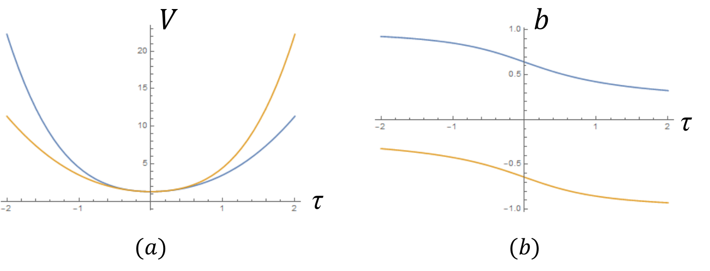
Refer to caption
Figure 1: (aa) Plots of two solutions V⁡(τ)V(\tau) of effective equation at ℰ=4\mathcal{E}=4, β=1\beta=1, κ=1\kappa=1. Each solution exhibits an unsymmetric bounce at τ=0\tau=0. The big-bang singularity is resolved by the bounce with nonzero volume Vc=1.29092V_{c}=1.29092. The solution represented by the blue curve reduces asymptotically to a solution to the Friedmann equation or Eq.181 as τ→∞\tau\to\infty and reduces to Eq.182 as τ→−∞\tau\to-\infty. The solution represented by the orange curve is given by a time refection. (b)(b) Plots of two corresponding b⁡(τ)b(\tau).

We can even obtain analytically solutions of b⁡(τ)b(\tau), which is going to be useful for computing semiclassical amplitude in the next section. From the (174),

V=93​ℰ3​β6​κ383​sin6⁡(b)​[−β2+8​(β2+1)​cos⁡(2​b)+8]3\displaystyle V=\frac{9^{3}\mathcal{E}^{3}\beta^{6}\kappa^{3}}{8^{3}\sin^{6}(b)\left[-\beta^{2}+8\left(\beta^{2}+1\right)\cos(2b)+8\right]^{3}} (185)

substitute into (173), we then have

d​bd​τ\displaystyle\frac{\mathrm{d}b}{\mathrm{d}\tau} =\displaystyle= −16​sin4⁡(b)​[−β2+8​(β2+1)​cos⁡(2​b)+8]2243​β3​κ\displaystyle-\frac{16\sin^{4}(b)\left[-\beta^{2}+8\left(\beta^{2}+1\right)\cos(2b)+8\right]^{2}}{243\beta^{3}\kappa} (186)

whose sulution is given by

b⁡(τ)=f−1​(c1+16​τ9​β3​ℰ​κ)\displaystyle b(\tau)=f^{-1}\left(c_{1}+\frac{16\tau}{9\beta^{3}\mathcal{E}\kappa}\right) (187)

where c1c_{1} is a integration constant and x=f−1​(y)x=f^{-1}(y) is the inverse function of f⁡(x)=yf(x)=y with f⁡(x)f(x) given by

f⁡(x)=\displaystyle f(x)= 18​(55​β2+64)​cot⁡(x)(7​β2+16)3−3072​(β2+1)3​sin⁡(2​x)β2​(7​β2+16)3​(−β2+8​(β2+1)​cos⁡(2​x)+8)\displaystyle\frac{18\left(55\beta^{2}+64\right)\cot(x)}{\left(7\beta^{2}+16\right)^{3}}-\frac{3072\left(\beta^{2}+1\right)^{3}\sin(2x)}{\beta^{2}\left(7\beta^{2}+16\right)^{3}\left(-\beta^{2}+8\left(\beta^{2}+1\right)\cos(2x)+8\right)} (188)
+9​cot⁡(x)​csc2⁡(x)(7​β2+16)2−256​(19​β2−8)​(β2+1)2β3​(7​β2+16)7/2​tanh−1⁡(3​β​tan⁡(x)7​β2+16)\displaystyle+\frac{9\cot(x)\csc^{2}(x)}{\left(7\beta^{2}+16\right)^{2}}-\frac{256\left(19\beta^{2}-8\right)\left(\beta^{2}+1\right)^{2}}{\beta^{3}\left(7\beta^{2}+16\right)^{7/2}}\tanh^{-1}\left(\frac{3\beta\tan(x)}{\sqrt{7\beta^{2}+16}}\right)

Solution of Eq.186 is unique once fixing the inital condition. With a suitable c1c_{1}, Eq.187 corresponds to the solution of the “+” branch in Eq.184 with sin⁡(b⁡(0))=14​7​β2+162​(β2+1)\sin(b(0))=\frac{1}{4}\sqrt{\frac{7\beta^{2}+16}{2(\beta^{2}+1)}}. The “-” branch corresponds to a different solution with sin⁡(b⁡(0))=−14​7​β2+162​(β2+1)\sin(b(0))=-\frac{1}{4}\sqrt{\frac{7\beta^{2}+16}{2(\beta^{2}+1)}}:

b⁡(τ)=−f−1​(c1−16​τ9​β3​ℰ​κ),\displaystyle b(\tau)=-f^{-1}\left(c_{1}-\frac{16\tau}{9\beta^{3}\mathcal{E}\kappa}\right), (189)

by observing that, (186) is invariant under simultaneously b→−bb\to-b and τ→−τ\tau\to-\tau. c1c_{1} is fixed to

c1=6​β​25​β2+16​(149​β4+112​β2−64)−256​(β2+1)2​(19​β2−8)​tanh−1⁡(3​β25​β2+16)β3​(7​β2+16)7/2.\displaystyle c_{1}=\frac{6\beta\sqrt{25\beta^{2}+16}\left(149\beta^{4}+112\beta^{2}-64\right)-256\left(\beta^{2}+1\right)^{2}\left(19\beta^{2}-8\right)\tanh^{-1}\left(\frac{3\beta}{\sqrt{25\beta^{2}+16}}\right)}{\beta^{3}\left(7\beta^{2}+16\right)^{7/2}}. (190)

Let’s briefly discuss the solutions from the AALM Hamiltonian given in (163). The equations of motion in this case are given by

d​Vd​τ\displaystyle\frac{\mathrm{d}V}{\mathrm{d}\tau} =\displaystyle= 2​V2/3​sin⁡(2​b)β,\displaystyle\frac{2V^{2/3}\sin(2b)}{\beta}, (191)
d​bd​τ\displaystyle\frac{\mathrm{d}b}{\mathrm{d}\tau} =\displaystyle= −2​sin2⁡(b)3​β​V1/3.\displaystyle-\frac{2\sin^{2}(b)}{3\beta V^{1/3}}. (192)

and the conserved physical Hamiltonian in the dust-time evolution:

𝐇|V⁡(γ)|=8​V1/3​sin2⁡(b)β2​κ=ρ​V≡ℰ.\displaystyle\frac{\mathbf{H}}{|V(\gamma)|}=\frac{8{V}^{1/3}\sin^{2}(b)}{\beta^{2}\kappa}=\rho V\equiv\mathcal{E}. (193)

All above discussions of solutions can be repeated analogously, so we skip the details. Two solutions b⁡(τ)b(\tau) are still given by (187) and (189), but with f⁡(x)f(x) given by:

f⁡(x)=\displaystyle f(x)= 19​cot⁡(x)​[2+csc2⁡(x)].\displaystyle\frac{1}{9}\cot(x)\left[2+\csc^{2}(x)\right]. (194)

where c1c_{1} is now fixed to c1=0c_{1}=0 with initial condition b⁡(0)=±π2b(0)=\pm\frac{\pi}{2}. In this case the two solutions V⁡(τ)V(\tau) become coincide, leading to the symmetric bounce as in the standard LQC. The critical values of bb and VV at the bounce are given by

b⁡(0)=±π2,Vc=ℰ3​β6​κ3512\displaystyle b(0)=\pm\frac{\pi}{2},\qquad V_{c}=\frac{\mathcal{E}^{3}\beta^{6}\kappa^{3}}{512} (195)

Solutions V⁡(τ),b⁡(τ)V(\tau),b(\tau) are plotted in FIG.2

Refer to caption
Figure 2: (aa) Plots of two solutions V⁡(τ)V(\tau) of effective equation from the AALM Hamiltonian, at ℰ=4\mathcal{E}=4, β=1\beta=1, κ=1\kappa=1. Two solutions V⁡(τ)V(\tau) coincide and exhibit a symmetric bounce at τ=0\tau=0. The big-bang singularity is resolved by the bounce with nonzero volume Vc=0.125V_{c}=0.125. Both solutions reduce asymptotically to a solution to the Friedmann equation as τ→±∞\tau\to\pm\infty. (b)(b) Plots of two corresponding b⁡(τ)b(\tau).

8 Semiclassical amplitude

Given the initial and final states Ψ[g]t,Ψ[g′]t\Psi^{t}_{[g]},\Psi^{t}_{[g^{\prime}]} in the amplitude A[g],[g′]A_{[g],[g^{\prime}]} in Eq.37. The semiclassical approximation of A[g],[g′]A_{[g],[g^{\prime}]} can be obtained by evaluating the integrand in the path integral Eq.44 at the solution of EOMs, i.e. up to prefactors including the integration measure and 1-loop determinant (determinant of Hessian),

A[g],[g′]‖ψgt‖​‖ψg′t‖∼eS⁡[g,h]/t|solution,\displaystyle\frac{A_{[g],[g^{\prime}]}}{||\psi^{t}_{g}||\,||{\psi}^{t}_{g^{\prime}}||}\sim e^{S[g,h]/t}\Big|_{\text{solution}}, (196)

provided that there exists a unique solution satisfying the initial and final conditions. If the initial and final condition do not fix uniquely a solution, the above gives the contribution to the semiclassica amplitude from one solution, while A[g],[g′]A_{[g],[g^{\prime}]} is approximated by summing over all solutions.

The solution in FIG.1 or 2 (with fixed initial and final conditions) is unique within the homogeneous and isotropic sector. The uniqueness of the solution in full theory will be studied in Han:2019unique.

We evaluate the on-shell action as follows: In the action (45), applying the homogeneous and isotropic ansatz Eq.79 to K⁡[gi+1,gi]K[g_{i+1},g_{i}] gives

K⁡[gi+1,gi]=\displaystyle K[g_{i+1},g_{i}]= −3​|V⁡(γ)|4​[(pi+1−pi)2+(θi+1−θi)2+2​i​(pi+pi+1)​(θi+1−θi)]\displaystyle-\frac{3|V(\gamma)|}{4}\Big[(p_{i+1}-p_{i})^{2}+(\theta_{i+1}-\theta_{i})^{2}+2{i}(p_{i}+p_{i+1})(\theta_{i+1}-\theta_{i})\Big]
=\displaystyle= −3​|V⁡(γ)|4​Δ​τ​[2​i​(pi+pi+1)​(θi+1−θi)Δ​τ+((pi+1−pi)2Δ​τ2+(θi+1−θi)2Δ​τ2)​Δ​τ]\displaystyle-\frac{3|V(\gamma)|}{4}\Delta\tau\left[2{i}(p_{i}+p_{i+1})\frac{(\theta_{i+1}-\theta_{i})}{\Delta\tau}+\Big(\frac{(p_{i+1}-p_{i})^{2}}{\Delta\tau^{2}}+\frac{(\theta_{i+1}-\theta_{i})^{2}}{\Delta\tau^{2}}\Big)\Delta\tau\right] (197)

In approximation Δ→0\Delta\to 0, the action becomes

S=−i|V(γ)|∫dτ(3pθ˙+κa2𝐇|V⁡(γ)|)=−i|V⁡(γ)|a2​β∫dτ(6V23b˙+κβ𝐇|V⁡(γ)|)\displaystyle S=-i|V(\gamma)|\int d\tau\Big(3p\dot{\theta}+\frac{\kappa}{a^{2}}\frac{\bf{H}}{|V(\gamma)|}\Big)=-i\frac{|V(\gamma)|}{a^{2}\beta}\int d\tau\Big({6V^{\frac{2}{3}}\dot{b}}+{\kappa}\beta\frac{\bf{H}}{|V(\gamma)|}\Big) (198)

where θ˙=d​θ​(τ)/d​τ\dot{\theta}={\mathrm{d}\theta(\tau)}/{\mathrm{d}\tau}. 𝐇|V⁡(γ)|\frac{\bf{H}}{|V(\gamma)|} is given by (174). The equation of motion implies

𝐇|V⁡(γ)|=−12​V23β​κ​d​bd​τ.\displaystyle\frac{{\bf H}}{|V(\gamma)|}=-\frac{12V^{\frac{2}{3}}}{\beta\kappa}\frac{db}{d\tau}. (199)

The action can be computed explicitly

S=\displaystyle S= i​6​|V⁡(γ)|a2​β​∫0Td​τ​b˙​V23=i​6​|V⁡(γ)|a2​β​∫b⁡(0)b⁡(T)d​b​V​(b)23\displaystyle i\frac{6|V(\gamma)|}{a^{2}\beta}\int_{0}^{T}d\,\tau\;\dot{b}V^{\frac{2}{3}}=i\frac{6|V(\gamma)|}{a^{2}\beta}\int_{b(0)}^{b(T)}d\,b\;V(b)^{\frac{2}{3}} (200)
=\displaystyle= i​6​|V⁡(γ)|a2​β​∫b⁡(0)b⁡(T)d​b​81​β4​ℰ2​κ264​sin4⁡(b)​[β2−8​(β2+1)​cos⁡(2​b)−8]2\displaystyle i\frac{6|V(\gamma)|}{a^{2}\beta}\int_{b(0)}^{b(T)}d\,{b}\;\frac{81\beta^{4}\mathcal{E}^{2}\kappa^{2}}{64\sin^{4}({b})\left[\beta^{2}-8\left(\beta^{2}+1\right)\cos(2{b})-8\right]^{2}} (201)
=\displaystyle= −i​9​|V⁡(γ)|​β3​ℰ2​κ232​a2​f​(b⁡(τ))|b⁡(0)b⁡(T)\displaystyle-i\frac{9|V(\gamma)|\beta^{3}\mathcal{E}^{2}\kappa^{2}}{32a^{2}}f\big(b(\tau)\big)\Bigg|_{b(0)}^{b(T)} (202)

where f⁡(x)f(x) is given in (188). Substitute the solution of b⁡(τ)b(\tau) into the action, we obtain SS is linear to TT

S=−i​κ​|V⁡(γ)|2​a2​ℰ​T\displaystyle S=-i\frac{\kappa|V(\gamma)|}{2a^{2}}\,\mathcal{E}T (203)

The above result is from the Giesel-Thiemann’s Hamiltonian. But interestingly the AALM Hamiltonian gives exactly the same expression as Eq.203.

9 Outlook: continuum limit, quantum effects, and μ¯\bar{\mu}-scheme

Although the effective equation derived from full LQG demonstrates the bounce resolving the big-bang singularity, the result has the same issue as the μ0\mu_{0}-scheme in LQC, i.e. the critical density ρc\rho_{c} and critical volume VcV_{c} depends on the conserved energy ℰ\mathcal{E}. It might seem that for large ℰ\mathcal{E}, the bounce could happen at arbitrarily low density or large volume.

Our expectation is that this issue should be resolved by taking into account the continuum limit and quantum effects in the path integral formula Eq.44. The role played by the continuum limit is suggested by Eq.174, where ℰ\mathcal{E} is the energy per lattice vertex, given by the total energy 𝐇{\bf H} divided by the total number of lattice sites |V⁡(γ)||V(\gamma)|. Heuristically, the continuum limit of the lattice γ\gamma, |V⁡(γ)|→∞|V(\gamma)|\to\infty, prevents large ℰ\mathcal{E} (thus prevents low ρc\rho_{c}) for any finite total energy 𝐇{\bf H}. But this argument is heuristic because Eq.174 with |V⁡(γ)|→∞|V(\gamma)|\to\infty would lead to ℰ→0\mathcal{E}\to 0 so Vc→0V_{c}\to 0, which contradicted the minimal area and volume gaps in LQG. We might introduce an effective cut-off ℰm​i​n\mathcal{E}_{min} or |V⁡(γ)|m​a​x|V(\gamma)|_{max} to regulate VcV_{c} from zero. But more systematically, when applying the continuum limit to the cosmological effective dynamics, we should take into account the quantum effects which is important in the deep Planck regime, and presumably, modifies Eq.174.

The LQC μ¯\bar{\mu}-scheme Ashtekar:2006wn; Assanioussi:2019iye suggests the following ad hoc modification in the Hamiltonian 𝐇{\bf H} in e.g. Eq.174,

V1/3→V,\displaystyle V^{1/3}\ \to\ V, (204)

and modify the Hamiltonian evolution equations Eqs.172 and 173 accordingly55 5 The corresponding modification of 𝐇{\bf H} in Eq.148 is 𝐇→−4​a3​|V⁡(γ)|κ​Δ​(2​β​p)3/2​[sin2⁡(θ)−49​1+β2β2​sin2⁡(2​θ)],\displaystyle{\bf H}\to-\frac{4a^{3}|V(\gamma)|}{\kappa\,\Delta}(2\beta p)^{3/2}\left[\sin^{2}(\theta)-\frac{4}{9}\frac{1+\beta^{2}}{\beta^{2}}\sin^{2}(2\theta)\right], (205) then the modified evolution equations can be derived from Eq.149. In order to balance the dimension in Eq.174, we have to add an area scale Δ\Delta in the denominator, i.e. we make the following modification

κ→κ​Δ\displaystyle\kappa\ \to\ \kappa\Delta (206)

in the denominator of Eq.174. A similar computation as in Section 7 shows that this ad hoc modification leads to the critical density

ρc=(7​β2+16)272​β2​(β2+1)​κ​Δ\displaystyle\rho_{c}=\frac{\left(7\beta^{2}+16\right)^{2}}{72\beta^{2}\left(\beta^{2}+1\right)\kappa\Delta} (207)

independent of the conserved energy ℰ\mathcal{E}. ρc\rho_{c} is Planckian if Δ\Delta is Planckian. The LQC μ¯\bar{\mu} scheme takes Δ\Delta to be the minimal LQG area eigenvalue.

We anticipate that the above modification should be explained by taking into account quantum effects in the path integral Eq.44 66 6 There is a recent work in Alesci:2016rmn where average over graphs is taken into count in computing the expectation value of Hamiltonian to relate the μ¯\bar{\mu}-scheme.. The μ¯\bar{\mu}-scheme should relate to the quantum effective EOM, which may be derived from the full quantum effective action of our path integral. As a preliminary idea, we know that a typical implication of quantum effects is the running of coupling constant with respect to energy scales. In the path integral of LQG, κ\kappa is the only coupling constant, while the energy scale relates to the length scale μ\mu in e.g. Eq.81, thus relates to the number of lattice sites |V⁡(γ)||V(\gamma)| (we may let μ=1/|V⁡(γ)|\mu=1/|V(\gamma)| in certain macroscopic unit). Thus the continuum limit |V⁡(γ)|→∞|V(\gamma)|\to\infty should run κ\kappa away from its infrared value. The running of κ\kappa seems to relate to the above ad hoc modification in Eq.206. The following conjectured β\beta-function of κ\kappa may lead to Eq.206 with Δ∼ℓP2\Delta\sim\ell^{2}_{P} when μ→ℓP\mu\to\ell_{P}:

β⁡(κ)=μ​dd​μ​κ=4​κ.\displaystyle\beta(\kappa)=\mu\frac{\mathrm{d}}{\mathrm{d}\mu}\kappa=4\kappa. (208)

κ\kappa scaling as μ4\mu^{4} might force V1/3→VV^{1/3}\ \to\ V in the effective Hamiltonian as above, since the scaling dimension of the Hamiltonian shouldn’t change by quantum effects.

The above argument depends on the conjectured running of κ\kappa, and assumes the effective Hamiltonian taking into account the quantum effects depends on bb in the same manner as in Eq.174. At the moment, we still don’t have good justifications of these assumptions from full LQG perspective. A systematic study requires to understand the quantum effective action of the path integral.

In addition to the above idea about μ¯\bar{\mu}-scheme, there are several other perspectives in which our work should be developed further:

  • •

    The effective equations 75, 76, and 77 are valid for full LQG, therefore should be applied to other situation such as black holes, gravitational waves, etc. It is especially interesting to study the effective dynamics with non-homogeneous space and its time evolution.

  • •

    The effective equations of full LQG is formulated to be suitable for numerical simulation. It is interesting to develop numerical techniques to solve the effective equations for complicated dynamical situations, and make contact with numerical relativity.

  • •

    In the path integral method the derivation do not requires a dynamically stable coherent states. However this strategy may relate to the proposal of stable coherent states, because the saddle point approximation of path integral shows that the transition amplitude between two coherent states are not suppressed (namely time evolution of one coherent state has a large overlap with the other) only when they are related by equations of motion. In this sense our proof is related to the question whether these coherent states are dynamically stable. It is useful to make the relation more precise in the future.

  • •

    Section 6.3 suggests that the AALM Hamiltonian with scalar curvature operator should relate to a simpler effective Hamiltonian. There are also some other recent results based on the simplicity of this Hamiltonian (see e.g. Kisielowski:2018oiv; Assanioussi:2017tql; Zhang:2019dgi. However as is mentioned in Section 6.3, the semiclassical limit of the scalar curvature operator has not yet been checked in the literature for the most general situation. Especially its expectation values with respect to coherent states used in this work has not been well studied yet. It is useful to spend some future work on the semiclassical limit of scalar curvature operator and the corresponding Hamiltonian.

Acknowledgements

The authors acknowledge Kristina Giesel, Andrea Dapor, Klaus Liegener, Yongge Ma, and Xiangdong Zhang for useful communications, and acknowledge Hui Luo and Ling-Yan Hung for sharing computational resources. This work receives support from the National Science Foundation through grants PHY-1602867 and PHY-1912278.

Appendix A Variations of S⁡[g,h]S[g,h]

A.1 Variations gi​(e)↦giε​(e)=gi​(e)​eεia​(e)​τai=1,⋯,N+1g_{i}(e)\mapsto g_{i}^{\varepsilon}(e)=g_{i}(e)e^{\varepsilon_{i}^{a}(e)\tau^{a}}\quad i=1,\cdots,N+1

First of all, the variation of xi+1,ix_{i+1,i} gives

xi+1,iε​(e)\displaystyle x_{i+1,i}^{\varepsilon}(e) =\displaystyle= 12Tr[gi+1ε†(e)giε(e)]=12Tr[e−εi+1a​(e)∗​τagi+1†(e)gi(e)eεia​(e)​τa]\displaystyle\frac{1}{2}\mathrm{Tr}\left[g_{i+1}^{\varepsilon\dagger}(e)g_{i}^{\varepsilon}(e)\right]=\frac{1}{2}\mathrm{Tr}\left[e^{-\varepsilon_{i+1}^{a}(e)^{*}\tau^{a}}g_{i+1}^{\dagger}(e)g_{i}(e)e^{\varepsilon_{i}^{a}(e)\tau^{a}}\right]
=\displaystyle= 12​Tr​[(1−εi+1a​(e)∗​τa)​gi+1†​(e)​gi​(e)​(1+εia​(e)​τa)]\displaystyle\frac{1}{2}\mathrm{Tr}\left[\left(1-\varepsilon_{i+1}^{a}(e)^{*}\tau^{a}\right)g_{i+1}^{\dagger}(e)g_{i}(e)\left(1+\varepsilon_{i}^{a}(e)\tau^{a}\right)\right]
=\displaystyle= 12​Tr​[gi+1†​(e)​gi​(e)]+εia​(e)2​Tr​[τa​gi+1†​(e)​gi​(e)]−εi+1a​(e)∗2​Tr​[τa​gi+1†​(e)​gi​(e)]+O⁡(ε2).\displaystyle\frac{1}{2}\mathrm{Tr}\left[g_{i+1}^{\dagger}(e)g_{i}(e)\right]+\frac{\varepsilon_{i}^{a}(e)}{2}\mathrm{Tr}\left[\tau^{a}g_{i+1}^{\dagger}(e)g_{i}(e)\right]-\frac{\varepsilon_{i+1}^{a}(e)^{*}}{2}\mathrm{Tr}\left[\tau^{a}g_{i+1}^{\dagger}(e)g_{i}(e)\right]+O(\varepsilon^{2}).

Since

zi+1,iε​(e)=arccosh⁡(xi+1,iε​(e)),∂zi+1,iε​(e)∂xi+1,iε​(e)=1xi+1,iε​(e)−1​xi+1,iε​(e)+1,z_{i+1,i}^{\varepsilon}(e)=\mathrm{arccosh}\left(x_{i+1,i}^{\varepsilon}(e)\right),\quad\frac{\partial z_{i+1,i}^{\varepsilon}(e)}{\partial x_{i+1,i}^{\varepsilon}(e)}=\frac{1}{\sqrt{x_{i+1,i}^{\varepsilon}(e)-1}\sqrt{x_{i+1,i}^{\varepsilon}(e)+1}},

we obtain that

δε​(zi+1,iε​(e)2)=εia​(e)​∂zi+1,iε​(e)2∂εia​(e)|ε=0+εi+1a​(e)∗​∂zi+1,iε​(e)2∂εi+1a​(e)∗|ε=0\displaystyle\delta_{\varepsilon}\left(z_{i+1,i}^{\varepsilon}(e)^{2}\right)=\varepsilon_{i}^{a}(e)\frac{\partial z_{i+1,i}^{\varepsilon}(e)^{2}}{\partial\varepsilon_{i}^{a}(e)}|_{\varepsilon=0}+\varepsilon_{i+1}^{a}(e)^{*}\frac{\partial z_{i+1,i}^{\varepsilon}(e)^{2}}{\partial\varepsilon_{i+1}^{a}(e)^{*}}|_{\varepsilon=0}
=2​εia​(e)​zi+1,i​(e)​∂zi+1,iε​(e)∂xi+1,iε​(e)​∂xi+1,iε​(e)∂εia​(e)|ε=0+2​εi+1a​(e)∗​zi+1,i​(e)​∂zi+1,iε​(e)∂xi+1,iε​(e)​∂xi+1,iε​(e)∂εi+1a​(e)∗|ε=0\displaystyle=2\varepsilon_{i}^{a}(e)z_{i+1,i}(e)\frac{\partial z_{i+1,i}^{\varepsilon}(e)}{\partial x_{i+1,i}^{\varepsilon}(e)}\frac{\partial x_{i+1,i}^{\varepsilon}(e)}{\partial\varepsilon_{i}^{a}(e)}|_{\varepsilon=0}+2\varepsilon_{i+1}^{a}(e)^{*}z_{i+1,i}(e)\frac{\partial z_{i+1,i}^{\varepsilon}(e)}{\partial x_{i+1,i}^{\varepsilon}(e)}\frac{\partial x_{i+1,i}^{\varepsilon}(e)}{\partial\varepsilon_{i+1}^{a}(e)^{*}}|_{\varepsilon=0}
=2​εia​(e)​zi+1,i​(e)xi+1,i​(e)−1​xi+1,i​(e)+1​12​Tr​[τa​gi+1†​(e)​gi​(e)]−2​εi+1a​(e)∗​zi+1,i​(e)xi+1,i​(e)−1​xi+1,i​(e)+1​12​Tr​[τa​gi+1†​(e)​gi​(e)]\displaystyle=\frac{2\varepsilon_{i}^{a}(e)z_{i+1,i}(e)}{\sqrt{x_{i+1,i}(e)-1}\sqrt{x_{i+1,i}(e)+1}}\frac{1}{2}\mathrm{Tr}\left[\tau^{a}g_{i+1}^{\dagger}(e)g_{i}(e)\right]-\frac{2\varepsilon_{i+1}^{a}(e)^{*}z_{i+1,i}(e)}{\sqrt{x_{i+1,i}(e)-1}\sqrt{x_{i+1,i}(e)+1}}\frac{1}{2}\mathrm{Tr}\left[\tau^{a}g_{i+1}^{\dagger}(e)g_{i}(e)\right]
=εia​(e)​zi+1,i​(e)xi+1,i​(e)−1​xi+1,i​(e)+1​Tr​[τa​gi+1†​(e)​gi​(e)]−εi+1a​(e)∗​zi+1,i​(e)xi+1,i​(e)−1​xi+1,i​(e)+1​Tr​[τa​gi+1†​(e)​gi​(e)].\displaystyle=\frac{\varepsilon_{i}^{a}(e)z_{i+1,i}(e)}{\sqrt{x_{i+1,i}(e)-1}\sqrt{x_{i+1,i}(e)+1}}\mathrm{Tr}\left[\tau^{a}g_{i+1}^{\dagger}(e)g_{i}(e)\right]-\frac{\varepsilon_{i+1}^{a}(e)^{*}z_{i+1,i}(e)}{\sqrt{x_{i+1,i}(e)-1}\sqrt{x_{i+1,i}(e)+1}}\mathrm{Tr}\left[\tau^{a}g_{i+1}^{\dagger}(e)g_{i}(e)\right].

Similarly

δε​(pi+1​(e)2)\displaystyle\delta_{\varepsilon}\left(p_{i+1}(e)^{2}\right) =\displaystyle= εi+1a​(e)​pi+1​(e)sinh⁡(pi+1​(e))​Tr​[τa​gi+1†​(e)​gi+1​(e)]−εi+1a​(e)∗​pi+1​(e)sinh⁡(pi+1​(e))​Tr​[τa​gi+1†​(e)​gi+1​(e)],\displaystyle\frac{\varepsilon_{i+1}^{a}(e)p_{i+1}(e)}{\sinh\left(p_{i+1}(e)\right)}\mathrm{Tr}\left[\tau^{a}g_{i+1}^{\dagger}(e)g_{i+1}(e)\right]-\frac{\varepsilon_{i+1}^{a}(e)^{*}p_{i+1}(e)}{\sinh\left(p_{i+1}(e)\right)}\mathrm{Tr}\left[\tau^{a}g_{i+1}^{\dagger}(e)g_{i+1}(e)\right],
δε​(pi​(e)2)\displaystyle\delta_{\varepsilon}\left(p_{i}(e)^{2}\right) =\displaystyle= εia​(e)​pi​(e)sinh⁡(pi​(e))​Tr​[τa​gi†​(e)​gi​(e)]−εia​(e)∗​pi​(e)sinh⁡(pi​(e))​Tr​[τa​gi†​(e)​gi​(e)],\displaystyle\frac{\varepsilon_{i}^{a}(e)p_{i}(e)}{\sinh\left(p_{i}(e)\right)}\mathrm{Tr}\left[\tau^{a}g_{i}^{\dagger}(e)g_{i}(e)\right]-\frac{\varepsilon_{i}^{a}(e)^{*}p_{i}(e)}{\sinh\left(p_{i}(e)\right)}\mathrm{Tr}\left[\tau^{a}g_{i}^{\dagger}(e)g_{i}(e)\right],

since pi+1​(e)>0p_{i+1}(e)>0

cosh⁡(pi+1​(e))−1​cosh⁡(pi+1​(e))+1=cosh⁡(pi+1​(e))2−1=sinh⁡(pi+1​(e))2=sinh⁡(pi+1​(e)).\sqrt{\cosh\left(p_{i+1}(e)\right)-1}\sqrt{\cosh\left(p_{i+1}(e)\right)+1}=\sqrt{\cosh\left(p_{i+1}(e)\right)^{2}-1}=\sqrt{\sinh\left(p_{i+1}(e)\right)^{2}}=\sinh\left(p_{i+1}(e)\right).

We apply the above relations to δ​S\delta S

δε​S​[g,h]\displaystyle\delta_{\varepsilon}S[g,h] =\displaystyle= ∑i=0N+1∑e∈E⁡(γ)[δε​(zi+1,i​(e)2)−12​δε​(pi+1​(e)2)−12​δε​(pi​(e)2)]−i​κa2​∑i=1NΔ​τ​[δε​⟨ψgi+1t|𝐇^|ψgit⟩⟨ψgi+1t|ψgit⟩]\displaystyle\sum_{i=0}^{N+1}\sum_{e\in E(\gamma)}\left[\delta_{\varepsilon}\left(z_{i+1,i}(e)^{2}\right)-\frac{1}{2}\delta_{\varepsilon}\left(p_{i+1}(e)^{2}\right)-\frac{1}{2}\delta_{\varepsilon}\left(p_{i}(e)^{2}\right)\right]-\frac{i\kappa}{a^{2}}\sum_{i=1}^{N}\Delta\tau\left[\delta_{\varepsilon}\frac{\langle\psi_{g_{i+1}}^{t}|\hat{\mathbf{H}}|\psi_{g_{i}}^{t}\rangle}{\langle\psi_{g_{i+1}}^{t}|\psi_{g_{i}}^{t}\rangle}\right]
=\displaystyle= ∑e∈E⁡(γ)∑i=0N+1(εia​(e)​zi+1,i​(e)xi+1,i​(e)−1​xi+1,i​(e)+1​Tr​[τa​gi+1†​(e)​gi​(e)]−εi+1a​(e)∗​zi+1,i​(e)xi+1,i​(e)−1​xi+1,i​(e)+1​Tr​[τa​gi+1†​(e)​gi​(e)]CLOSE\displaystyle\sum_{e\in E(\gamma)}\sum_{i=0}^{N+1}\Bigg(\frac{\varepsilon_{i}^{a}(e)z_{i+1,i}(e)}{\sqrt{x_{i+1,i}(e)-1}\sqrt{x_{i+1,i}(e)+1}}\mathrm{Tr}\left[\tau^{a}g_{i+1}^{\dagger}(e)g_{i}(e)\right]-\frac{\varepsilon_{i+1}^{a}(e)^{*}z_{i+1,i}(e)}{\sqrt{x_{i+1,i}(e)-1}\sqrt{x_{i+1,i}(e)+1}}\mathrm{Tr}\left[\tau^{a}g_{i+1}^{\dagger}(e)g_{i}(e)\right]
−12​εi+1a​(e)​pi+1​(e)sinh⁡(pi+1​(e))​Tr​[τa​gi+1†​(e)​gi+1​(e)]+12​εi+1a​(e)∗​pi+1​(e)sinh⁡(pi+1​(e))​Tr​[τa​gi+1†​(e)​gi+1​(e)]\displaystyle-\frac{1}{2}\frac{\varepsilon_{i+1}^{a}(e)p_{i+1}(e)}{\sinh\left(p_{i+1}(e)\right)}\mathrm{Tr}\left[\tau^{a}g_{i+1}^{\dagger}(e)g_{i+1}(e)\right]+\frac{1}{2}\frac{\varepsilon_{i+1}^{a}(e)^{*}p_{i+1}(e)}{\sinh\left(p_{i+1}(e)\right)}\mathrm{Tr}\left[\tau^{a}g_{i+1}^{\dagger}(e)g_{i+1}(e)\right]
OPEN−12​εia​(e)​pi​(e)sinh⁡(pi​(e))​Tr​[τa​gi†​(e)​gi​(e)]+12​εia​(e)∗​pi​(e)sinh⁡(pi​(e))​Tr​[τa​gi†​(e)​gi​(e)])\displaystyle-\frac{1}{2}\frac{\varepsilon_{i}^{a}(e)p_{i}(e)}{\sinh\left(p_{i}(e)\right)}\mathrm{Tr}\left[\tau^{a}g_{i}^{\dagger}(e)g_{i}(e)\right]+\frac{1}{2}\frac{\varepsilon_{i}^{a}(e)^{*}p_{i}(e)}{\sinh\left(p_{i}(e)\right)}\mathrm{Tr}\left[\tau^{a}g_{i}^{\dagger}(e)g_{i}(e)\right]\Bigg)
−i​κa2∑i=1NΔτ[∑e∈E⁡(γ)εia(e)∂∂εia​(e)⟨ψgi+1εt|𝐇^|ψgiεt⟩⟨ψgi+1εt|ψgiεt⟩|ε=0+∑e∈E⁡(γ)εi+1a(e)∗∂∂εi+1a​(e)∗⟨ψgi+1εt|𝐇^|ψgiεt⟩⟨ψgi+1εt|ψgiεt⟩|ε=0]\displaystyle-\frac{i\kappa}{a^{2}}\sum_{i=1}^{N}\Delta\tau\left[\sum_{e\in E(\gamma)}\varepsilon_{i}^{a}(e)\frac{\partial}{\partial\varepsilon_{i}^{a}(e)}\frac{\langle\psi_{g_{i+1}^{\varepsilon}}^{t}|\hat{\mathbf{H}}|\psi_{g_{i}^{\varepsilon}}^{t}\rangle}{\langle\psi_{g_{i+1}^{\varepsilon}}^{t}|\psi_{g_{i}^{\varepsilon}}^{t}\rangle}|_{\varepsilon=0}+\sum_{e\in E(\gamma)}\varepsilon_{i+1}^{a}(e)^{*}\frac{\partial}{\partial\varepsilon_{i+1}^{a}(e)^{*}}\frac{\langle\psi_{g_{i+1}^{\varepsilon}}^{t}|\hat{\mathbf{H}}|\psi_{g_{i}^{\varepsilon}}^{t}\rangle}{\langle\psi_{g_{i+1}^{\varepsilon}}^{t}|\psi_{g_{i}^{\varepsilon}}^{t}\rangle}|_{\varepsilon=0}\right]
=\displaystyle= ∑e∈E⁡(γ)∑i=1N+1εia​(e)​(zi+1,i​(e)xi+1,i​(e)−1​xi+1,i​(e)+1​Tr​[τa​gi+1†​(e)​gi​(e)]−pi​(e)sinh⁡(pi​(e))​Tr​[τa​gi†​(e)​gi​(e)])\displaystyle\sum_{e\in E(\gamma)}\sum_{i=1}^{N+1}\varepsilon_{i}^{a}(e)\Bigg(\frac{z_{i+1,i}(e)}{\sqrt{x_{i+1,i}(e)-1}\sqrt{x_{i+1,i}(e)+1}}\mathrm{Tr}\left[\tau^{a}g_{i+1}^{\dagger}(e)g_{i}(e)\right]-\frac{p_{i}(e)}{\sinh\left(p_{i}(e)\right)}\mathrm{Tr}\left[\tau^{a}g_{i}^{\dagger}(e)g_{i}(e)\right]\Bigg)
+∑e∈E⁡(γ)∑i=1N+1εia(e)∗(−zi,i−1​(e)xi,i−1​(e)−1​xi,i−1​(e)+1Tr[τagi†(e)gi−1(e)]+pi​(e)sinh⁡(pi​(e))Tr[τagi†(e)gi(e)])\displaystyle+\sum_{e\in E(\gamma)}\sum_{i=1}^{N+1}\varepsilon_{i}^{a}(e)^{*}\Bigg(-\frac{z_{i,i-1}(e)}{\sqrt{x_{i,i-1}(e)-1}\sqrt{x_{i,i-1}(e)+1}}\mathrm{Tr}\left[\tau^{a}g_{i}^{\dagger}(e)g_{i-1}(e)\right]+\frac{p_{i}(e)}{\sinh\left(p_{i}(e)\right)}\mathrm{Tr}\left[\tau^{a}g_{i}^{\dagger}(e)g_{i}(e)\right]\Bigg)
−i​κ​Δ​τa2∑e∈E⁡(γ)[∑i=1Nεia(e)∂∂εia​(e)⟨ψgi+1εt|𝐇^|ψgiεt⟩⟨ψgi+1εt|ψgiεt⟩|ε=0+∑i=2N+1εia(e)∗∂∂εia​(e)∗⟨ψgiεt|𝐇^|ψgi−1εt⟩⟨ψgiεt|ψgi−1εt⟩|ε=0]\displaystyle-\frac{i\kappa\Delta\tau}{a^{2}}\sum_{e\in E(\gamma)}\left[\sum_{i=1}^{N}\varepsilon_{i}^{a}(e)\frac{\partial}{\partial\varepsilon_{i}^{a}(e)}\frac{\langle\psi_{g_{i+1}^{\varepsilon}}^{t}|\hat{\mathbf{H}}|\psi_{g_{i}^{\varepsilon}}^{t}\rangle}{\langle\psi_{g_{i+1}^{\varepsilon}}^{t}|\psi_{g_{i}^{\varepsilon}}^{t}\rangle}|_{\varepsilon=0}+\sum_{i=2}^{N+1}\varepsilon_{i}^{a}(e)^{*}\frac{\partial}{\partial\varepsilon_{i}^{a}(e)^{*}}\frac{\langle\psi_{g_{i}^{\varepsilon}}^{t}|\hat{\mathbf{H}}|\psi_{g_{i-1}^{\varepsilon}}^{t}\rangle}{\langle\psi_{g_{i}^{\varepsilon}}^{t}|\psi_{g_{i-1}^{\varepsilon}}^{t}\rangle}|_{\varepsilon=0}\right]

where ε0a​(e)=εN+2a​(e)=0\varepsilon_{0}^{a}(e)=\varepsilon_{N+2}^{a}(e)=0 in the 2nd step.

We can extract the following EOMs:
For i=1,⋯,Ni=1,\cdots,N,

δ​Sδ​εia​(e)=0:zi+1,i​(e)​Tr​[τa​gi+1†​(e)​gi​(e)]xi+1,i​(e)−1​xi+1,i​(e)+1−pi​(e)​Tr​[τa​gi†​(e)​gi​(e)]sinh⁡(pi​(e))=i​κ​Δ​τa2​∂∂εia​(e)​⟨ψgi+1εt|𝐇^|ψgiεt⟩⟨ψgi+1εt|ψgiεt⟩|ε=0\frac{\delta S}{\delta\varepsilon_{i}^{a}(e)}=0:\quad\frac{z_{i+1,i}(e)\mathrm{Tr}\left[\tau^{a}g_{i+1}^{\dagger}(e)g_{i}(e)\right]}{\sqrt{x_{i+1,i}(e)-1}\sqrt{x_{i+1,i}(e)+1}}-\frac{p_{i}(e)\mathrm{Tr}\left[\tau^{a}g_{i}^{\dagger}(e)g_{i}(e)\right]}{\sinh\left(p_{i}(e)\right)}=\frac{i\kappa\Delta\tau}{a^{2}}\frac{\partial}{\partial\varepsilon_{i}^{a}(e)}\frac{\langle\psi_{g_{i+1}^{\varepsilon}}^{t}|\hat{\mathbf{H}}|\psi_{g_{i}^{\varepsilon}}^{t}\rangle}{\langle\psi_{g_{i+1}^{\varepsilon}}^{t}|\psi_{g_{i}^{\varepsilon}}^{t}\rangle}\Bigg|_{\varepsilon=0}

For i=N+1i=N+1

δ​Sδ​εN+1a​(e)=0:zN+2,N+1​(e)​Tr​[τa​gN+2†​(e)​gN+1​(e)]xN+2,N+1​(e)−1​xN+2,N+1​(e)+1−pN+1​(e)​Tr​[τa​gN+1†​(e)​gN+1​(e)]sinh⁡(pN+1​(e))=0.\frac{\delta S}{\delta\varepsilon_{N+1}^{a}(e)}=0:\quad\frac{z_{N+2,N+1}(e)\mathrm{Tr}\left[\tau^{a}g_{N+2}^{\dagger}(e)g_{N+1}(e)\right]}{\sqrt{x_{N+2,N+1}(e)-1}\sqrt{x_{N+2,N+1}(e)+1}}-\frac{p_{N+1}(e)\mathrm{Tr}\left[\tau^{a}g_{N+1}^{\dagger}(e)g_{N+1}(e)\right]}{\sinh\left(p_{N+1}(e)\right)}=0.

For i=2,⋯,N+1i=2,\cdots,N+1,

δ​Sδ​εia​(e)∗=0:zi,i−1​(e)​Tr​[τa​gi†​(e)​gi−1​(e)]xi,i−1​(e)−1​xi,i−1​(e)+1−pi​(e)​Tr​[τa​gi†​(e)​gi​(e)]sinh⁡(pi​(e))=−i​κ​Δ​τa2​∂∂εia​(e)∗​⟨ψgiεt|𝐇^|ψgi−1εt⟩⟨ψgiεt|ψgi−1εt⟩|ε=0.\frac{\delta S}{\delta\varepsilon_{i}^{a}(e)^{*}}=0:\quad\frac{z_{i,i-1}(e)\mathrm{Tr}\left[\tau^{a}g_{i}^{\dagger}(e)g_{i-1}(e)\right]}{\sqrt{x_{i,i-1}(e)-1}\sqrt{x_{i,i-1}(e)+1}}-\frac{p_{i}(e)\mathrm{Tr}\left[\tau^{a}g_{i}^{\dagger}(e)g_{i}(e)\right]}{\sinh\left(p_{i}(e)\right)}=-\frac{i\kappa\Delta\tau}{a^{2}}\frac{\partial}{\partial\varepsilon_{i}^{a}(e)^{*}}\frac{\langle\psi_{g_{i}^{\varepsilon}}^{t}|\hat{\mathbf{H}}|\psi_{g_{i-1}^{\varepsilon}}^{t}\rangle}{\langle\psi_{g_{i}^{\varepsilon}}^{t}|\psi_{g_{i-1}^{\varepsilon}}^{t}\rangle}\Bigg|_{\varepsilon=0}.

For i=1i=1

δ​Sδ​ε1a​(e)∗=0:z10​(e)​Tr​[τa​g1†​(e)​g0​(e)]x10​(e)−1​x10​(e)+1−p1​(e)​Tr​[τa​g1†​(e)​g1​(e)]sinh⁡(p1​(e))=0.\frac{\delta S}{\delta\varepsilon_{1}^{a}(e)^{*}}=0:\quad\frac{z_{10}(e)\mathrm{Tr}\left[\tau^{a}g_{1}^{\dagger}(e)g_{0}(e)\right]}{\sqrt{x_{10}(e)-1}\sqrt{x_{10}(e)+1}}-\frac{p_{1}(e)\mathrm{Tr}\left[\tau^{a}g_{1}^{\dagger}(e)g_{1}(e)\right]}{\sinh\left(p_{1}(e)\right)}=0.

A.2 Variation hvη=hv​eηva​τa​ with ​ηva∈ℝh_{v}^{\eta}=h_{v}e^{\eta_{v}^{a}\tau^{a}}\text{ with }\eta_{v}^{a}\in\mathbb{R}

Firstly the variation of g′hg^{\prime h} gives

g0​(e)\displaystyle g_{0}(e) =g′hη​(e)=hs⁡(e)η,−1​g′​(e)​ht⁡(e)η=e−ηs⁡(e)a​τa​hs⁡(e)−1​g′​(e)​ht⁡(e)​eηt⁡(e)a​τa\displaystyle=g^{\prime h^{\eta}}(e)=h_{s(e)}^{\eta,-1}g^{\prime}(e)h_{t(e)}^{\eta}=e^{-\eta_{s(e)}^{a}\tau^{a}}h_{s(e)}^{-1}g^{\prime}(e)h_{t(e)}e^{\eta_{t(e)}^{a}\tau^{a}}
=(1−ηs⁡(e)a​τa)​hs⁡(e)−1​g′​(e)​ht⁡(e)​(1+ηt⁡(e)a​τa)+O⁡(η2)\displaystyle=\left(1-\eta_{s(e)}^{a}\tau^{a}\right)h_{s(e)}^{-1}g^{\prime}(e)h_{t(e)}\left(1+\eta_{t(e)}^{a}\tau^{a}\right)+O\left(\eta^{2}\right)
=(1−ηs⁡(e)a​τa)​g′h​(e)​(1+ηt⁡(e)a​τa)+O⁡(η2)\displaystyle=\left(1-\eta_{s(e)}^{a}\tau^{a}\right)g^{\prime h}(e)\left(1+\eta_{t(e)}^{a}\tau^{a}\right)+O\left(\eta^{2}\right)

The variation of x10​(e)x_{10}(e) can be computed

x10η​(e)\displaystyle x_{10}^{\eta}(e) =12​Tr​[g1†​(e)​g0η​(e)]=12​Tr​[g1†​(e)​g′hη​(e)]\displaystyle=\frac{1}{2}\mathrm{Tr}\left[g_{1}^{\dagger}(e)g_{0}^{\eta}(e)\right]=\frac{1}{2}\mathrm{Tr}\left[g_{1}^{\dagger}(e)g^{\prime h^{\eta}}(e)\right]
=12​Tr​[g1†​(e)​(1−ηs⁡(e)a​τa)​g′h​(e)​(1+ηt⁡(e)a​τa)]+O⁡(η2)\displaystyle=\frac{1}{2}\mathrm{Tr}\left[g_{1}^{\dagger}(e)\left(1-\eta_{s(e)}^{a}\tau^{a}\right)g^{\prime h}(e)\left(1+\eta_{t(e)}^{a}\tau^{a}\right)\right]+O\left(\eta^{2}\right)
=12​Tr​[g1†​(e)​g′h​(e)]+ηt⁡(e)a2​Tr​[τa​g1†​(e)​g′h​(e)]−ηs⁡(e)a2​Tr​[g1†​(e)​τa​g′h​(e)]+O⁡(η2).\displaystyle=\frac{1}{2}\mathrm{Tr}\left[g_{1}^{\dagger}(e)g^{\prime h}(e)\right]+\frac{\eta_{t(e)}^{a}}{2}\mathrm{Tr}\left[\tau^{a}g_{1}^{\dagger}(e)g^{\prime h}(e)\right]-\frac{\eta_{s(e)}^{a}}{2}\mathrm{Tr}\left[g_{1}^{\dagger}(e)\tau^{a}g^{\prime h}(e)\right]+O\left(\eta^{2}\right).

Moreover,

x0η​(e)\displaystyle x_{0}^{\eta}(e) ≡12Tr[g0η†(e)g0η(e)]=12Tr[g′hη(e)†g′hη(e)]\displaystyle\equiv\frac{1}{2}\mathrm{Tr}\left[g_{0}^{\eta\dagger}(e)g_{0}^{\eta}(e)\right]=\frac{1}{2}\mathrm{Tr}\left[g^{\prime h^{\eta}}(e)^{\dagger}g^{\prime h^{\eta}}(e)\right]
=12​Tr​[(e−ηt⁡(e)a​τa​ht⁡(e)†​g′​(e)†​hs⁡(e)​eηs⁡(e)a​τa)​(e−ηs⁡(e)a​τa​hs⁡(e)−1​g′​(e)​ht⁡(e)​eηt⁡(e)a​τa)]\displaystyle=\frac{1}{2}\mathrm{Tr}\left[\left(e^{-\eta_{t(e)}^{a}\tau^{a}}h_{t(e)}^{\dagger}g^{\prime}(e)^{\dagger}h_{s(e)}e^{\eta_{s(e)}^{a}\tau^{a}}\right)\left(e^{-\eta_{s(e)}^{a}\tau^{a}}h_{s(e)}^{-1}g^{\prime}(e)h_{t(e)}e^{\eta_{t(e)}^{a}\tau^{a}}\right)\right]
=12​Tr​[(ht⁡(e)†​g′​(e)†​hs⁡(e))​(hs⁡(e)−1​g′​(e)​ht⁡(e))]\displaystyle=\frac{1}{2}\mathrm{Tr}\left[\left(h_{t(e)}^{\dagger}g^{\prime}(e)^{\dagger}h_{s(e)}\right)\left(h_{s(e)}^{-1}g^{\prime}(e)h_{t(e)}\right)\right]
=x0​(e).\displaystyle=x_{0}(e).

Therefore we have

δη​x10​(e)=ηt⁡(e)a2​Tr​[τa​g1†​(e)​g′h​(e)]−ηs⁡(e)a2​Tr​[g1†​(e)​τa​g′h​(e)]\delta_{\eta}x_{10}(e)=\frac{\eta_{t(e)}^{a}}{2}\mathrm{Tr}\left[\tau^{a}g_{1}^{\dagger}(e)g^{\prime h}(e)\right]-\frac{\eta_{s(e)}^{a}}{2}\mathrm{Tr}\left[g_{1}^{\dagger}(e)\tau^{a}g^{\prime h}(e)\right]
δη​x0​(e)=0⇒δη​p0​(e)=0.\delta_{\eta}x_{0}(e)=0\quad\Rightarrow\quad\delta_{\eta}p_{0}(e)=0.

Then we compute δη​(z10​(e)2)\delta_{\eta}\left(z_{10}(e)^{2}\right):

δη​(z10​(e)2)\displaystyle\delta_{\eta}\left(z_{10}(e)^{2}\right) =2​z10​(e)​δη​z10​(e)=2​z10​(e)​∂z10​(e)∂x10​(e)​δη​x10​(e)\displaystyle=2z_{10}(e)\delta_{\eta}z_{10}(e)=2z_{10}(e)\frac{\partial z_{10}(e)}{\partial x_{10}(e)}\delta_{\eta}x_{10}(e)
=2​z10​(e)x10​(e)−1​x10​(e)+1​(ηt⁡(e)a2​Tr​[τa​g1†​(e)​g′h​(e)]−ηs⁡(e)a2​Tr​[g1†​(e)​τa​g′h​(e)])\displaystyle=\frac{2z_{10}(e)}{\sqrt{x_{10}(e)-1}\sqrt{x_{10}(e)+1}}\left(\frac{\eta_{t(e)}^{a}}{2}\mathrm{Tr}\left[\tau^{a}g_{1}^{\dagger}(e)g^{\prime h}(e)\right]-\frac{\eta_{s(e)}^{a}}{2}\mathrm{Tr}\left[g_{1}^{\dagger}(e)\tau^{a}g^{\prime h}(e)\right]\right)
=z10​(e)x10​(e)−1​x10​(e)+1​(ηt⁡(e)a​Tr​[τa​g1†​(e)​g′h​(e)]−ηs⁡(e)a​Tr​[g1†​(e)​τa​g′h​(e)]).\displaystyle=\frac{z_{10}(e)}{\sqrt{x_{10}(e)-1}\sqrt{x_{10}(e)+1}}\left(\eta_{t(e)}^{a}\mathrm{Tr}\left[\tau^{a}g_{1}^{\dagger}(e)g^{\prime h}(e)\right]-\eta_{s(e)}^{a}\mathrm{Tr}\left[g_{1}^{\dagger}(e)\tau^{a}g^{\prime h}(e)\right]\right).

Applying the above results to the variation of S⁡[g,h]S[g,h] gives

δη​S​[g,h]\displaystyle\delta_{\eta}S[g,h] =∑e∈E⁡(γ)[δη​z10​(e)2]\displaystyle=\sum_{e\in E(\gamma)}\left[\delta_{\eta}z_{10}(e)^{2}\right]
=∑e∈E⁡(γ)z10​(e)x10​(e)−1​x10​(e)+1​(ηt⁡(e)a​Tr​[τa​g1†​(e)​g′h​(e)]−ηs⁡(e)a​Tr​[g1†​(e)​τa​g′h​(e)]),\displaystyle=\sum_{e\in E(\gamma)}\frac{z_{10}(e)}{\sqrt{x_{10}(e)-1}\sqrt{x_{10}(e)+1}}\left(\eta_{t(e)}^{a}\mathrm{Tr}\left[\tau^{a}g_{1}^{\dagger}(e)g^{\prime h}(e)\right]-\eta_{s(e)}^{a}\mathrm{Tr}\left[g_{1}^{\dagger}(e)\tau^{a}g^{\prime h}(e)\right]\right),

which leads to the following variation equation:

δ​S​[g,h]δ​ηva=∑e,t⁡(e)=vz10​(e)​Tr​[τa​g1†​(e)​g′h​(e)]x10​(e)−1​x10​(e)+1−∑e,s⁡(e)=vz10​(e)​Tr​[g1†​(e)​τa​g′h​(e)]x10​(e)−1​x10​(e)+1=0.\frac{\delta S[g,h]}{\delta\eta_{v}^{a}}=\sum_{e,t(e)=v}\frac{z_{10}(e)\mathrm{Tr}\left[\tau^{a}g_{1}^{\dagger}(e)g^{\prime h}(e)\right]}{\sqrt{x_{10}(e)-1}\sqrt{x_{10}(e)+1}}-\sum_{e,s(e)=v}\frac{z_{10}(e)\mathrm{Tr}\left[g_{1}^{\dagger}(e)\tau^{a}g^{\prime h}(e)\right]}{\sqrt{x_{10}(e)-1}\sqrt{x_{10}(e)+1}}=0.

When we impose the initial condition g1=g′hg_{1}=g^{\prime h}, we obtain

z10​(e)=p1​(e),x10​(e)=cosh⁡(p1​(e)),x10​(e)−1​x10​(e)+1=cosh⁡(p1​(e))2−1=sinh⁡(p1​(e)),z_{10}(e)=p_{1}(e),\quad x_{10}(e)=\cosh\left(p_{1}(e)\right),\quad\sqrt{x_{10}(e)-1}\sqrt{x_{10}(e)+1}=\sqrt{\cosh\left(p_{1}(e)\right)^{2}-1}=\sinh\left(p_{1}(e)\right),

and the following simplifications:

Tr⁡[τa​g1†​(e)​g′h​(e)]\displaystyle\mathrm{Tr}\left[\tau^{a}g_{1}^{\dagger}(e)g^{\prime h}(e)\right] =Tr[τag1†(e)g1(e)]=Tr[τae−θaτa/2e−ipaτa/2e−ipaτa/2eθa​τa/2]\displaystyle=\mathrm{Tr}\left[\tau^{a}g_{1}^{\dagger}(e)g_{1}(e)\right]=\mathrm{Tr}\left[\tau^{a}e^{-\theta^{a}\tau^{a}/2}e^{-ip^{a}\tau^{a}/2}e^{-ip^{a}\tau^{a}/2}e^{\theta^{a}\tau^{a}/2}\right]
=Tr[eθa​τa/2τae−θaτa/2e−i​pa​τa]=Λba(θ)Tr[τbe−i​pc​τc]\displaystyle=\mathrm{Tr}\left[e^{\theta^{a}\tau^{a}/2}\tau^{a}e^{-\theta^{a}\tau^{a}/2}e^{-ip^{a}\tau^{a}}\right]=\Lambda_{\ b}^{a}(\theta)\mathrm{Tr}\left[\tau^{b}e^{-ip^{c}\tau^{c}}\right]
=Λba​(θ)​Tr​[τb​(cosh⁡(p)−i​pc​τcp​sinh⁡(p))]\displaystyle=\Lambda_{\ b}^{a}(\theta)\mathrm{Tr}\left[\tau^{b}\left(\cosh(p)-i\frac{p^{c}\tau^{c}}{p}\sinh(p)\right)\right]
=−i​pcp​sinh⁡(p)​Λba​(θ)​Tr​[τb​τc]\displaystyle=-i\frac{p^{c}}{p}\sinh(p)\Lambda_{\ b}^{a}(\theta)\mathrm{Tr}\left[\tau^{b}\tau^{c}\right]
=2​i​sinh⁡(p)p​Λca​(θ)​pc,\displaystyle=2i\frac{\sinh(p)}{p}\Lambda_{\ c}^{a}(\theta)p^{c},

where eθa​τa/2τae−θaτa/2=Λba(θ)τbe^{\theta^{a}\tau^{a}/2}\tau^{a}e^{-\theta^{a}\tau^{a}/2}=\Lambda_{\ b}^{a}\mathrm{(\theta)}\tau^{b}. Similarly,

Tr⁡[g1†​(e)​τa​g′h​(e)]\displaystyle\mathrm{Tr}\left[g_{1}^{\dagger}(e)\tau^{a}g^{\prime h}(e)\right] =Tr[g1†(e)τag1(e)]=Tr[e−θaτa/2e−ipaτa/2τae−ipaτa/2eθa​τa/2]\displaystyle=\mathrm{Tr}\left[g_{1}^{\dagger}(e)\tau^{a}g_{1}(e)\right]=\mathrm{Tr}\left[e^{-\theta^{a}\tau^{a}/2}e^{-ip^{a}\tau^{a}/2}\tau^{a}e^{-ip^{a}\tau^{a}/2}e^{\theta^{a}\tau^{a}/2}\right]
=Tr⁡[τa​e−i​pa​τa]=Tr⁡[τa​(cosh⁡(p)−i​pc​τcp​sinh⁡(p))]\displaystyle=\mathrm{Tr}\left[\tau^{a}e^{-ip^{a}\tau^{a}}\right]=\mathrm{Tr}\left[\tau^{a}\left(\cosh(p)-i\frac{p^{c}\tau^{c}}{p}\sinh(p)\right)\right]
=−i​pcp​sinh⁡(p)​Tr​[τa​τc]\displaystyle=-i\frac{p^{c}}{p}\sinh(p)\mathrm{Tr}\left[\tau^{a}\tau^{c}\right]
=2​i​sinh⁡(p)p​pa.\displaystyle=2i\frac{\sinh(p)}{p}p^{a}.

The variation equation reduces to

0=δ​S​[g,h]δ​ηva\displaystyle 0=\frac{\delta S[g,h]}{\delta\eta_{v}^{a}} =∑e,t⁡(e)=vp1​(e)​2​i​sinh⁡(p⁡(e))p⁡(e)​Λca​(θ)​pc​(e)sinh⁡(p1​(e))−∑e,s⁡(e)=vp1​(e)​2​i​sinh⁡(p⁡(e))p⁡(e)​pa​(e)sinh⁡(p1​(e))\displaystyle=\sum_{e,t(e)=v}\frac{p_{1}(e)2i\frac{\sinh(p(e))}{p(e)}\Lambda_{\ c}^{a}(\theta)p^{c}(e)}{\sinh\left(p_{1}(e)\right)}-\sum_{e,s(e)=v}\frac{p_{1}(e)2i\frac{\sinh(p(e))}{p(e)}p^{a}(e)}{\sinh\left(p_{1}(e)\right)}
=∑e,t⁡(e)=v2​i​Λca​(θ)​pc​(e)−∑e,s⁡(e)=v2​i​pa​(e).\displaystyle=\sum_{e,t(e)=v}2i\Lambda_{\ c}^{a}(\theta)p^{c}(e)-\sum_{e,s(e)=v}2ip^{a}(e).

Appendix B Derivation in Lemma 4.1

B.1 D1a​(gi,gj)D_{1}^{a}(g_{i},g_{j})

We apply gi=gj​[1+Δ​ϕa​τa+O⁡(Δ​ϕ2)]g_{i}=g_{j}\left[1+\Delta\phi^{a}\tau^{a}+O\left(\Delta\phi^{2}\right)\right] to

D1a​(gi,gj)\displaystyle D_{1}^{a}(g_{i},g_{j}) =\displaystyle= zi​jxi​j−1​xi​j+1​Tr​[τa​gi†​gj]−pjsinh⁡(pj)​Tr​[τa​gj†​gj].\displaystyle\frac{z_{ij}}{\sqrt{x_{ij}-1}\sqrt{x_{ij}+1}}\mathrm{Tr}\left[\tau^{a}g_{i}^{\dagger}g_{j}\right]-\frac{p_{j}}{\sinh\left(p_{j}\right)}\mathrm{Tr}\left[\tau^{a}g_{j}^{\dagger}g_{j}\right].

We use the following relations: Firstly,

xi​j\displaystyle x_{ij} =12​Tr​[gi†​gj]=12​Tr​[[1+Δ​ϕa​τa+O⁡(Δ​ϕ2)]†​gj†​gj]\displaystyle=\frac{1}{2}\mathrm{Tr}\left[g_{i}^{\dagger}g_{j}\right]=\frac{1}{2}\mathrm{Tr}\left[\left[1+\Delta\phi^{a}\tau^{a}+O\left(\Delta\phi^{2}\right)\right]^{\dagger}g_{j}^{\dagger}g_{j}\right]
=12Tr[[1−Δϕa∗τa]gj†gj]+O(Δϕ2)\displaystyle=\frac{1}{2}\mathrm{Tr}\left[\left[1-\Delta\phi^{a*}\tau^{a}\right]g_{j}^{\dagger}g_{j}\right]+O\left(\Delta\phi^{2}\right)
=12Tr[gj†gj]−12Δϕa∗Tr[τagj†gj]+O(Δϕ2)\displaystyle=\frac{1}{2}\mathrm{Tr}\left[g_{j}^{\dagger}g_{j}\right]-\frac{1}{2}\Delta\phi^{a*}\mathrm{Tr}\left[\tau^{a}g_{j}^{\dagger}g_{j}\right]+O\left(\Delta\phi^{2}\right)
=cosh(pj)−iΔϕa∗sinh⁡(pj)pjΛca(θj)pjc++O(Δϕ2).\displaystyle=\cosh(p_{j})-i\Delta\phi^{a*}\frac{\sinh(p_{j})}{p_{j}}\Lambda_{\ c}^{a}(\theta_{j})p_{j}^{c}++O\left(\Delta\phi^{2}\right).

Secondly, since zi​j=arccosh⁡(xi​j)z_{ij}=\mathrm{arccosh}\left(x_{ij}\right),

δ​zi​j\displaystyle\delta z_{ij} =\displaystyle= ∂zi​j∂xi​j|gi=gj​δ​xi​j=δ​xi​jxi​j−1​xi​j+1|gi=gj\displaystyle\frac{\partial z_{ij}}{\partial x_{ij}}\Big|_{g_{i}=g_{j}}\delta x_{ij}=\frac{\delta x_{ij}}{\sqrt{x_{ij}-1}\sqrt{x_{ij}+1}}\Big|_{g_{i}=g_{j}}
=\displaystyle= 1sinh⁡(pj)[−iΔϕa∗sinh⁡(pj)pjΛca(θj)pjc]=−iΔϕa∗Λca(θj)pjcpj.\displaystyle\frac{1}{\sinh(p_{j})}\left[-i\Delta\phi^{a*}\frac{\sinh(p_{j})}{p_{j}}\Lambda_{\ c}^{a}(\theta_{j})p_{j}^{c}\right]=-i\Delta\phi^{a*}\Lambda_{\ c}^{a}(\theta_{j})\frac{p_{j}^{c}}{p_{j}}.

Thirdly,

Tr⁡[τa​gi†​gj]\displaystyle\mathrm{Tr}\left[\tau^{a}g_{i}^{\dagger}g_{j}\right] =\displaystyle= Tr[τa[1−Δϕa∗τa]gj†gj]\displaystyle\mathrm{Tr}\left[\tau^{a}\left[1-\Delta\phi^{a*}\tau^{a}\right]g_{j}^{\dagger}g_{j}\right]
=\displaystyle= Tr[τagj†gj]−Δϕb∗Tr[τaτbgj†gj]\displaystyle\mathrm{Tr}\left[\tau^{a}g_{j}^{\dagger}g_{j}\right]-\Delta\phi^{b*}\mathrm{Tr}\left[\tau^{a}\tau^{b}g_{j}^{\dagger}g_{j}\right]
=\displaystyle= Tr[τagj†gj]−Δϕb∗Tr[τaτbe−θjaτa/2e−i​pja​τaeθja​τa/2]\displaystyle\mathrm{Tr}\left[\tau^{a}g_{j}^{\dagger}g_{j}\right]-\Delta\phi^{b*}\mathrm{Tr}\left[\tau^{a}\tau^{b}e^{-\theta_{j}^{a}\tau^{a}/2}e^{-ip_{j}^{a}\tau^{a}}e^{\theta_{j}^{a}\tau^{a}/2}\right]
=\displaystyle= Tr[τagj†gj]−Δϕb∗Tr[eθja​τa/2τae−θjaτa/2eθja​τa/2τbe−θjaτa/2e−i​pja​τa]\displaystyle\mathrm{Tr}\left[\tau^{a}g_{j}^{\dagger}g_{j}\right]-\Delta\phi^{b*}\mathrm{Tr}\left[e^{\theta_{j}^{a}\tau^{a}/2}\tau^{a}e^{-\theta_{j}^{a}\tau^{a}/2}e^{\theta_{j}^{a}\tau^{a}/2}\tau^{b}e^{-\theta_{j}^{a}\tau^{a}/2}e^{-ip_{j}^{a}\tau^{a}}\right]
=\displaystyle= Tr[τagj†gj]−Δϕb∗Λca(θj)Λdb(θj)Tr[τcτd(cosh(pj)−ipje​τepjsinh(pj))]\displaystyle\mathrm{Tr}\left[\tau^{a}g_{j}^{\dagger}g_{j}\right]-\Delta\phi^{b*}\Lambda_{\ c}^{a}(\theta_{j})\Lambda_{\ d}^{b}(\theta_{j})\mathrm{Tr}\left[\tau^{c}\tau^{d}\left(\cosh(p_{j})-i\frac{p_{j}^{e}\tau^{e}}{p_{j}}\sinh(p_{j})\right)\right]
=\displaystyle= Tr[τagj†gj]−Δϕb∗Λca(θj)Λdb(θj)(−2δc​dcosh(pj)+2ipjepjsinh(pj)εc​d​e).\displaystyle\mathrm{Tr}\left[\tau^{a}g_{j}^{\dagger}g_{j}\right]-\Delta\phi^{b*}\Lambda_{\ c}^{a}(\theta_{j})\Lambda_{\ d}^{b}(\theta_{j})\left(-2\delta^{cd}\cosh(p_{j})+2i\frac{p_{j}^{e}}{p_{j}}\sinh(p_{j})\varepsilon^{cde}\right).

where we have used Tr⁡[τb​τc]=−Tr⁡[σb​σc]=−2​δb​c\mathrm{Tr}\left[\tau^{b}\tau^{c}\right]=-\mathrm{Tr}\left[\sigma^{b}\sigma^{c}\right]=-2\delta^{bc} and Tr⁡[τa​τb​τc]=i​Tr​[σa​σb​σc]=i⁡(2​i​εa​b​c)=−2​εa​b​c\mathrm{Tr}\left[\tau^{a}\tau^{b}\tau^{c}\right]=i\mathrm{Tr}\left[\sigma^{a}\sigma^{b}\sigma^{c}\right]=i(2i\varepsilon^{abc})=-2\varepsilon^{abc}.

Applying above relations to D1a​(gi,gj)D_{1}^{a}(g_{i},g_{j}) gives

D1a​(gi,gj)\displaystyle D_{1}^{a}(g_{i},g_{j})
=pj−iΔϕa∗Λca(θj)pjcpj[cosh(pj)−1][1−iΔϕa∗sinh⁡(pj)pj​[cosh⁡(pj)−1]Λca(θj)pjc]​[cosh(pj)+1][1−iΔϕa∗sinh⁡(pj)pj​[cosh⁡(pj)+1]Λca(θj)pjc]\displaystyle=\frac{p_{j}-i\Delta\phi^{a*}\Lambda_{\ c}^{a}(\theta_{j})\frac{p_{j}^{c}}{p_{j}}}{\sqrt{\left[\cosh(p_{j})-1\right]\left[1-i\Delta\phi^{a*}\frac{\sinh(p_{j})}{p_{j}\left[\cosh(p_{j})-1\right]}\Lambda_{\ c}^{a}(\theta_{j})p_{j}^{c}\right]}\sqrt{\left[\cosh(p_{j})+1\right]\left[1-i\Delta\phi^{a*}\frac{\sinh(p_{j})}{p_{j}\left[\cosh(p_{j})+1\right]}\Lambda_{\ c}^{a}(\theta_{j})p_{j}^{c}\right]}}
(Tr[τagj†gj]−Δϕb∗Λca(θj)Λdb(θj)(−2δc​dcosh(pj)+2ipjepjsinh(pj)εc​d​e))−pjsinh⁡(pj)Tr[τagj†gj]\displaystyle\left(\mathrm{Tr}\left[\tau^{a}g_{j}^{\dagger}g_{j}\right]-\Delta\phi^{b*}\Lambda_{\ c}^{a}(\theta_{j})\Lambda_{\ d}^{b}(\theta_{j})\left(-2\delta^{cd}\cosh(p_{j})+2i\frac{p_{j}^{e}}{p_{j}}\sinh(p_{j})\varepsilon^{cde}\right)\right)-\frac{p_{j}}{\sinh\left(p_{j}\right)}\mathrm{Tr}\left[\tau^{a}g_{j}^{\dagger}g_{j}\right]
=[pj−iΔϕa∗Λca(θj)pjcpj][1+iΔϕa∗sinh⁡(pj)2​pj​[cosh⁡(pj)−1]Λca(θj)pjc][1+iΔϕa∗sinh⁡(pj)2​pj​[cosh⁡(pj)+1]Λca(θj)pjc]sinh⁡(pj)\displaystyle=\frac{\left[p_{j}-i\Delta\phi^{a*}\Lambda_{\ c}^{a}(\theta_{j})\frac{p_{j}^{c}}{p_{j}}\right]\left[1+i\Delta\phi^{a*}\frac{\sinh(p_{j})}{2p_{j}\left[\cosh(p_{j})-1\right]}\Lambda_{\ c}^{a}(\theta_{j})p_{j}^{c}\right]\left[1+i\Delta\phi^{a*}\frac{\sinh(p_{j})}{2p_{j}\left[\cosh(p_{j})+1\right]}\Lambda_{\ c}^{a}(\theta_{j})p_{j}^{c}\right]}{\sinh(p_{j})}
(Tr[τagj†gj]−Δϕb∗Λca(θj)Λdb(θj)(−2δc​dcosh(pj)+2ipjepjsinh(pj)εc​d​e))−pjsinh⁡(pj)Tr[τagj†gj]\displaystyle\left(\mathrm{Tr}\left[\tau^{a}g_{j}^{\dagger}g_{j}\right]-\Delta\phi^{b*}\Lambda_{\ c}^{a}(\theta_{j})\Lambda_{\ d}^{b}(\theta_{j})\left(-2\delta^{cd}\cosh(p_{j})+2i\frac{p_{j}^{e}}{p_{j}}\sinh(p_{j})\varepsilon^{cde}\right)\right)-\frac{p_{j}}{\sinh\left(p_{j}\right)}\mathrm{Tr}\left[\tau^{a}g_{j}^{\dagger}g_{j}\right]
=−iΔϕa∗Λca(θj)pjc(1sinh⁡(pj)​pj−12​[cosh⁡(pj)−1]−12​[cosh⁡(pj)+1])2isinh⁡(pj)pjΛca(θj)pjc\displaystyle=-i\Delta\phi^{a*}\Lambda_{\ c}^{a}(\theta_{j})p_{j}^{c}\left(\frac{1}{\sinh(p_{j})p_{j}}-\frac{1}{2\left[\cosh(p_{j})-1\right]}-\frac{1}{2\left[\cosh(p_{j})+1\right]}\right)2i\frac{\sinh(p_{j})}{p_{j}}\Lambda_{\ c}^{a}(\theta_{j})p_{j}^{c}
−Δϕb∗Λca(θj)Λdb(θj)(−2δc​dcosh(pj)+2ipjepjsinh(pj)εc​d​e)pjsinh⁡(pj)\displaystyle-\Delta\phi^{b*}\Lambda_{\ c}^{a}(\theta_{j})\Lambda_{\ d}^{b}(\theta_{j})\left(-2\delta^{cd}\cosh(p_{j})+2i\frac{p_{j}^{e}}{p_{j}}\sinh(p_{j})\varepsilon^{cde}\right)\frac{p_{j}}{\sinh(p_{j})}
=2Δϕb∗Λca(θj)Λdb(θj)(pjcpjpjdpj−pjcpjpjdpjcosh⁡(pj)​pjsinh⁡(pj)+δc​dcosh⁡(pj)​pjsinh⁡(pj)−ipjeεc​d​e).\displaystyle=2\Delta\phi^{b*}\Lambda_{\ c}^{a}(\theta_{j})\Lambda_{\ d}^{b}(\theta_{j})\left(\frac{p_{j}^{c}}{p_{j}}\frac{p_{j}^{d}}{p_{j}}-\frac{p_{j}^{c}}{p_{j}}\frac{p_{j}^{d}}{p_{j}}\frac{\cosh(p_{j})p_{j}}{\sinh(p_{j})}+\delta^{cd}\frac{\cosh(p_{j})p_{j}}{\sinh(p_{j})}-ip_{j}^{e}\varepsilon^{cde}\right).

B.2 D2a​(gi,gj)D_{2}^{a}(g_{i},g_{j})

We apply gj=gi​[1−Δ​ϕa​τa+O⁡(Δ​ϕ2)]g_{j}=g_{i}\left[1-\Delta\phi^{a}\tau^{a}+O\left(\Delta\phi^{2}\right)\right] to

D2a​(gi,gj)=zi​jxi​j−1​xi​j+1​Tr​[τa​gi†​gj]−pisinh⁡(pi)​Tr​[τa​gi†​gi].D_{2}^{a}(g_{i},g_{j})=\frac{z_{ij}}{\sqrt{x_{ij}-1}\sqrt{x_{ij}+1}}\mathrm{Tr}\left[\tau^{a}g_{i}^{\dagger}g_{j}\right]-\frac{p_{i}}{\sinh\left(p_{i}\right)}\mathrm{Tr}\left[\tau^{a}g_{i}^{\dagger}g_{i}\right].

We use the following relations: Firstly,

xi​j\displaystyle x_{ij} =12​Tr​[gi†​gj]=12​Tr​[gi†​gi​[1−Δ​ϕa​τa]]+O⁡(Δ​ϕ2)\displaystyle=\frac{1}{2}\mathrm{Tr}\left[g_{i}^{\dagger}g_{j}\right]=\frac{1}{2}\mathrm{Tr}\left[g_{i}^{\dagger}g_{i}\left[1-\Delta\phi^{a}\tau^{a}\right]\right]+O\left(\Delta\phi^{2}\right)
=12​Tr​[gi†​gi]−12​Δ​ϕa​Tr​[τa​gi†​gi]+O⁡(Δ​ϕ2)\displaystyle=\frac{1}{2}\mathrm{Tr}\left[g_{i}^{\dagger}g_{i}\right]-\frac{1}{2}\Delta\phi^{a}\mathrm{Tr}\left[\tau^{a}g_{i}^{\dagger}g_{i}\right]+O\left(\Delta\phi^{2}\right)
=cosh⁡(pi)−i​Δ​ϕa​sinh⁡(pi)pi​Λca​(θi)​pic+O⁡(Δ​ϕ2).\displaystyle=\cosh(p_{i})-i\Delta\phi^{a}\frac{\sinh(p_{i})}{p_{i}}\Lambda_{\ c}^{a}(\theta_{i})p_{i}^{c}+O\left(\Delta\phi^{2}\right).

Secondly,

δ​zi​j=1sinh⁡(pj)​[−i​Δ​ϕa​sinh⁡(pi)pi​Λca​(θi)​pic]=−i​Δ​ϕa​Λca​(θi)​picpi.\delta z_{ij}=\frac{1}{\sinh(p_{j})}\left[-i\Delta\phi^{a}\frac{\sinh(p_{i})}{p_{i}}\Lambda_{\ c}^{a}(\theta_{i})p_{i}^{c}\right]=-i\Delta\phi^{a}\Lambda_{\ c}^{a}(\theta_{i})\frac{p_{i}^{c}}{p_{i}}.

Thridly,

Tr⁡[τa​gi†​gj]\displaystyle\mathrm{Tr}\left[\tau^{a}g_{i}^{\dagger}g_{j}\right] =\displaystyle= Tr⁡[[1−Δ​ϕb​τb]​τa​gi†​gi]\displaystyle\mathrm{Tr}\left[\left[1-\Delta\phi^{b}\tau^{b}\right]\tau^{a}g_{i}^{\dagger}g_{i}\right]
=\displaystyle= Tr⁡[τa​gi†​gi]−Δ​ϕb​Tr​[τb​τa​gi†​gi]\displaystyle\mathrm{Tr}\left[\tau^{a}g_{i}^{\dagger}g_{i}\right]-\Delta\phi^{b}\mathrm{Tr}\left[\tau^{b}\tau^{a}g_{i}^{\dagger}g_{i}\right]
=\displaystyle= Tr[τagi†gi]−ΔϕbTr[τbτae−θiaτa/2e−i​pia​τaeθia​τa/2]\displaystyle\mathrm{Tr}\left[\tau^{a}g_{i}^{\dagger}g_{i}\right]-\Delta\phi^{b}\mathrm{Tr}\left[\tau^{b}\tau^{a}e^{-\theta_{i}^{a}\tau^{a}/2}e^{-ip_{i}^{a}\tau^{a}}e^{\theta_{i}^{a}\tau^{a}/2}\right]
=\displaystyle= Tr⁡[τa​gi†​gi]−Δ​ϕb​Λdb​(θi)​Λca​(θi)​Tr​[τd​τc​(cosh⁡(pi)−i​pie​τepi​sinh⁡(pi))]\displaystyle\mathrm{Tr}\left[\tau^{a}g_{i}^{\dagger}g_{i}\right]-\Delta\phi^{b}\Lambda_{\ d}^{b}(\theta_{i})\Lambda_{\ c}^{a}(\theta_{i})\mathrm{Tr}\left[\tau^{d}\tau^{c}\left(\cosh(p_{i})-i\frac{p_{i}^{e}\tau^{e}}{p_{i}}\sinh(p_{i})\right)\right]
=\displaystyle= Tr⁡[τa​gi†​gi]−Δ​ϕb​Λca​(θj)​Λdb​(θj)​Tr​[τd​τc​(cosh⁡(pi)−i​pie​τepi​sinh⁡(pi))]\displaystyle\mathrm{Tr}\left[\tau^{a}g_{i}^{\dagger}g_{i}\right]-\Delta\phi^{b}\Lambda_{\ c}^{a}(\theta_{j})\Lambda_{\ d}^{b}(\theta_{j})\mathrm{Tr}\left[\tau^{d}\tau^{c}\left(\cosh(p_{i})-i\frac{p_{i}^{e}\tau^{e}}{p_{i}}\sinh(p_{i})\right)\right]
=\displaystyle= Tr⁡[τa​gi†​gi]−Δ​ϕb​Λca​(θj)​Λdb​(θj)​(−2​δc​d​cosh⁡(pi)−2​i​piepi​sinh⁡(pi)​εc​d​e).\displaystyle\mathrm{Tr}\left[\tau^{a}g_{i}^{\dagger}g_{i}\right]-\Delta\phi^{b}\Lambda_{\ c}^{a}(\theta_{j})\Lambda_{\ d}^{b}(\theta_{j})\left(-2\delta^{cd}\cosh(p_{i})-2i\frac{p_{i}^{e}}{p_{i}}\sinh(p_{i})\varepsilon^{cde}\right).

Applying above relations to D2a​(gi,gj)D_{2}^{a}(g_{i},g_{j}) gives

D2a​(gi,gj)\displaystyle D_{2}^{a}(g_{i},g_{j})
=pi−i​Δ​ϕa​Λca​(θi)​picpi[cosh⁡(pi)−1]​[1−i​Δ​ϕa​sinh⁡(pi)pi​[cosh⁡(pi)−1]​Λca​(θi)​pic]​[cosh⁡(pi)+1]​[1−i​Δ​ϕa​sinh⁡(pi)pi​[cosh⁡(pi)+1]​Λca​(θi)​pic]\displaystyle=\frac{p_{i}-i\Delta\phi^{a}\Lambda_{\ c}^{a}(\theta_{i})\frac{p_{i}^{c}}{p_{i}}}{\sqrt{\left[\cosh(p_{i})-1\right]\left[1-i\Delta\phi^{a}\frac{\sinh(p_{i})}{p_{i}\left[\cosh(p_{i})-1\right]}\Lambda_{\ c}^{a}(\theta_{i})p_{i}^{c}\right]}\sqrt{\left[\cosh(p_{i})+1\right]\left[1-i\Delta\phi^{a}\frac{\sinh(p_{i})}{p_{i}\left[\cosh(p_{i})+1\right]}\Lambda_{\ c}^{a}(\theta_{i})p_{i}^{c}\right]}}
[Tr[τagi†gi]−Δϕb∗Λca(θj)Λdb(θj)(−2δc​dcosh(pi)−2ipiepisinh(pi)εc​d​e)]−pisinh⁡(pi)Tr[τagi†gi]\displaystyle\left[\mathrm{Tr}\left[\tau^{a}g_{i}^{\dagger}g_{i}\right]-\Delta\phi^{b*}\Lambda_{\ c}^{a}(\theta_{j})\Lambda_{\ d}^{b}(\theta_{j})\left(-2\delta^{cd}\cosh(p_{i})-2i\frac{p_{i}^{e}}{p_{i}}\sinh(p_{i})\varepsilon^{cde}\right)\right]-\frac{p_{i}}{\sinh\left(p_{i}\right)}\mathrm{Tr}\left[\tau^{a}g_{i}^{\dagger}g_{i}\right]
=[pi−i​Δ​ϕb​Λdb​(θi)​pidpi]​[1+i​Δ​ϕb​sinh⁡(pi)2​pi​[cosh⁡(pi)−1]​Λdb​(θi)​pid]​[1+i​Δ​ϕb​sinh⁡(pi)2​pi​[cosh⁡(pi)+1]​Λdb​(θi)​pid][cosh⁡(pi)−1]​[cosh⁡(pi)+1]\displaystyle=\frac{\left[p_{i}-i\Delta\phi^{b}\Lambda_{\ d}^{b}(\theta_{i})\frac{p_{i}^{d}}{p_{i}}\right]\left[1+i\Delta\phi^{b}\frac{\sinh(p_{i})}{2p_{i}\left[\cosh(p_{i})-1\right]}\Lambda_{\ d}^{b}(\theta_{i})p_{i}^{d}\right]\left[1+i\Delta\phi^{b}\frac{\sinh(p_{i})}{2p_{i}\left[\cosh(p_{i})+1\right]}\Lambda_{\ d}^{b}(\theta_{i})p_{i}^{d}\right]}{\sqrt{\left[\cosh(p_{i})-1\right]}\sqrt{\left[\cosh(p_{i})+1\right]}}
[Tr[τagi†gi]−Δϕb∗Λca(θj)Λdb(θj)(−2δc​dcosh(pi)−2ipiepisinh(pi)εc​d​e)]−pisinh⁡(pi)Tr[τagi†gi]\displaystyle\left[\mathrm{Tr}\left[\tau^{a}g_{i}^{\dagger}g_{i}\right]-\Delta\phi^{b*}\Lambda_{\ c}^{a}(\theta_{j})\Lambda_{\ d}^{b}(\theta_{j})\left(-2\delta^{cd}\cosh(p_{i})-2i\frac{p_{i}^{e}}{p_{i}}\sinh(p_{i})\varepsilon^{cde}\right)\right]-\frac{p_{i}}{\sinh\left(p_{i}\right)}\mathrm{Tr}\left[\tau^{a}g_{i}^{\dagger}g_{i}\right]
=2​Δ​ϕb​sinh⁡(pi)pi​Λca​(θi)​Λdb​(θi)​pic​pid​(1sinh⁡(pi)​pi−cosh⁡(pi)sinh⁡(pi)2)\displaystyle=2\Delta\phi^{b}\frac{\sinh(p_{i})}{p_{i}}\Lambda_{\ c}^{a}(\theta_{i})\Lambda_{\ d}^{b}(\theta_{i})p_{i}^{c}p_{i}^{d}\left(\frac{1}{\sinh(p_{i})p_{i}}-\frac{\cosh(p_{i})}{\sinh(p_{i})^{2}}\right)
+2​Δ​ϕb​Λca​(θj)​Λdb​(θj)​(δc​d​cosh⁡(pi)+i​piepi​sinh⁡(pi)​εc​d​e)​pisinh⁡(pi)\displaystyle+2\Delta\phi^{b}\Lambda_{\ c}^{a}(\theta_{j})\Lambda_{\ d}^{b}(\theta_{j})\left(\delta^{cd}\cosh(p_{i})+i\frac{p_{i}^{e}}{p_{i}}\sinh(p_{i})\varepsilon^{cde}\right)\frac{p_{i}}{\sinh(p_{i})}
=2​Δ​ϕb​Λca​(θi)​Λdb​(θi)​(picpi​pidpi−pi​cosh⁡(pi)sinh⁡(pi)​picpi​pidpi+δc​d​pi​cosh⁡(pi)sinh⁡(pi)+i​pie​εc​d​e).\displaystyle=2\Delta\phi^{b}\Lambda_{\ c}^{a}(\theta_{i})\Lambda_{\ d}^{b}(\theta_{i})\left(\frac{p_{i}^{c}}{p_{i}}\frac{p_{i}^{d}}{p_{i}}-\frac{p_{i}\cosh(p_{i})}{\sinh(p_{i})}\frac{p_{i}^{c}}{p_{i}}\frac{p_{i}^{d}}{p_{i}}+\delta^{cd}\frac{p_{i}\cosh(p_{i})}{\sinh(p_{i})}+ip_{i}^{e}\varepsilon^{cde}\right).

References

  • (1) T. Thiemann, Modern Canonical Quantum General Relativity. Cambridge University Press, 2007.
  • (2) M. Han, W. Huang, and Y. Ma, Fundamental structure of loop quantum gravity, Int.J.Mod.Phys. D16 (2007) 1397–1474, [gr-qc/0509064].
  • (3) A. Ashtekar and J. Lewandowski, Background independent quantum gravity: A Status report, Class.Quant.Grav. 21 (2004) R53, [gr-qc/0404018].
  • (4) M. Bojowald, Absence of singularity in loop quantum cosmology, Phys. Rev. Lett. 86 (2001) 5227–5230, [gr-qc/0102069].
  • (5) A. Ashtekar, T. Pawlowski, and P. Singh, Quantum Nature of the Big Bang: Improved dynamics, Phys. Rev. D74 (2006) 084003, [gr-qc/0607039].
  • (6) A. Ashtekar, T. Pawlowski, and P. Singh, Quantum nature of the big bang, Phys. Rev. Lett. 96 (2006) 141301, [gr-qc/0602086].
  • (7) P. Singh, Are loop quantum cosmos never singular?, Class. Quant. Grav. 26 (2009) 125005, [arXiv:0901.2750].
  • (8) M. Assanioussi, A. Dapor, K. Liegener, and T. Pawlowski, Emergent de Sitter epoch of the Loop Quantum Cosmos: a detailed analysis, arXiv:1906.05315.
  • (9) A. Ashtekar, J. Olmedo, and P. Singh, Quantum extension of the Kruskal spacetime, Phys. Rev. D98 (2018), no. 12 126003, [arXiv:1806.02406].
  • (10) A. Ashtekar, J. Olmedo, and P. Singh, Quantum Transfiguration of Kruskal Black Holes, Phys. Rev. Lett. 121 (2018), no. 24 241301, [arXiv:1806.00648].
  • (11) M. Assanioussi, A. Dapor, and K. Liegener, Perspectives on the dynamics in loop effective black hole interior, arXiv:1908.05756.
  • (12) R. Gambini, J. Olmedo, and J. Pullin, Quantum black holes in Loop Quantum Gravity, Class. Quant. Grav. 31 (2014) 095009, [arXiv:1310.5996].
  • (13) J. Ben Achour, F. Lamy, H. Liu, and K. Noui, Polymer Schwarzschild black hole: An effective metric, EPL 123 (2018), no. 2 20006, [arXiv:1803.01152].
  • (14) M. Bojowald, S. Brahma, and D.-h. Yeom, Effective line elements and black-hole models in canonical loop quantum gravity, Phys. Rev. D98 (2018), no. 4 046015, [arXiv:1803.01119].
  • (15) N. Bodendorfer, F. M. Mele, and J. Münch, Effective Quantum Extended Spacetime of Polymer Schwarzschild Black Hole, Class. Quant. Grav. 36 (2019), no. 19 195015, [arXiv:1902.04542].
  • (16) C. Rovelli and F. Vidotto, Planck stars, Int. J. Mod. Phys. D23 (2014), no. 12 1442026, [arXiv:1401.6562].
  • (17) M. Han and M. Zhang, Spinfoams near a classical curvature singularity, Phys. Rev. D94 (2016), no. 10 104075, [arXiv:1606.02826].
  • (18) M. Bojowald, Loop quantum cosmology, Living Rev. Rel. 8 (2005) 11, [gr-qc/0601085].
  • (19) A. Ashtekar, Loop Quantum Cosmology: An Overview, Gen. Rel. Grav. 41 (2009) 707–741, [arXiv:0812.0177].
  • (20) I. Agullo and P. Singh, Loop Quantum Cosmology, in Loop Quantum Gravity: The First 30 Years (A. Ashtekar and J. Pullin, eds.), pp. 183–240. WSP, 2017. arXiv:1612.01236.
  • (21) V. Taveras, Corrections to the Friedmann Equations from LQG for a Universe with a Free Scalar Field, Phys. Rev. D78 (2008) 064072, [arXiv:0807.3325].
  • (22) M. Bojowald, The BKL scenario, infrared renormalization, and quantum cosmology, JCAP 1901 (2019), no. 01 026, [arXiv:1810.00238].
  • (23) E. Alesci and F. Cianfrani, Quantum-Reduced Loop Gravity: Cosmology, Phys. Rev. D87 (2013), no. 8 083521, [arXiv:1301.2245].
  • (24) N. Bodendorfer, Quantum reduction to Bianchi I models in loop quantum gravity, Phys. Rev. D91 (2015), no. 8 081502, [arXiv:1410.5608].
  • (25) N. Bodendorfer, An embedding of loop quantum cosmology in (b,v)(b,v) variables into a full theory context, Class. Quant. Grav. 33 (2016), no. 12 125014, [arXiv:1512.00713].
  • (26) E. Alesci and F. Cianfrani, Improved regularization from Quantum Reduced Loop Gravity, arXiv:1604.02375.
  • (27) A. Dapor and K. Liegener, Cosmological Effective Hamiltonian from full Loop Quantum Gravity Dynamics, Phys. Lett. B785 (2018) 506–510, [arXiv:1706.09833].
  • (28) J. Engle, Relating loop quantum cosmology to loop quantum gravity: Symmetric sectors and embeddings, Class. Quant. Grav. 24 (2007) 5777–5802, [gr-qc/0701132].
  • (29) M. Hanusch, Invariant Connections and Symmetry Reduction in Loop Quantum Gravity, arXiv e-prints (Jan, 2016) arXiv:1601.05531, [arXiv:1601.05531].
  • (30) C. Fleischhack, Loop Quantization and Symmetry: Configuration Spaces, Commun. Math. Phys. 360 (2018), no. 2 481–521, [arXiv:1010.0449].
  • (31) C. Rovelli and F. Vidotto, Stepping out of Homogeneity in Loop Quantum Cosmology, Class. Quant. Grav. 25 (2008) 225024, [arXiv:0805.4585].
  • (32) K. Giesel and T. Thiemann, Algebraic quantum gravity (AQG). IV. Reduced phase space quantisation of loop quantum gravity, Class. Quant. Grav. 27 (2010) 175009, [arXiv:0711.0119].
  • (33) K. Giesel and T. Thiemann, Scalar Material Reference Systems and Loop Quantum Gravity, Class. Quant. Grav. 32 (2015) 135015, [arXiv:1206.3807].
  • (34) J. D. Brown and K. V. Kuchar, Dust as a standard of space and time in canonical quantum gravity, Phys. Rev. D51 (1995) 5600–5629, [gr-qc/9409001].
  • (35) K. V. Kuchar and C. G. Torre, Gaussian reference fluid and interpretation of quantum geometrodynamics, Phys. Rev. D43 (1991) 419–441.
  • (36) M. Domagala, K. Giesel, W. Kaminski, and J. Lewandowski, Gravity quantized: Loop Quantum Gravity with a Scalar Field, Phys. Rev. D82 (2010) 104038, [arXiv:1009.2445].
  • (37) C. Rovelli and L. Smolin, The Physical Hamiltonian in nonperturbative quantum gravity, Phys. Rev. Lett. 72 (1994) 446–449, [gr-qc/9308002].
  • (38) T. Thiemann, Quantum spin dynamics (QSD), Class. Quant. Grav. 15 (1998) 839–873, [gr-qc/9606089].
  • (39) E. Alesci, M. Assanioussi, J. Lewandowski, and I. Makinen, Hamiltonian operator for loop quantum gravity coupled to a scalar field, Phys. Rev. D91 (2015), no. 12 124067, [arXiv:1504.02068].
  • (40) M. Assanioussi, J. Lewandowski, and I. Makinen, New scalar constraint operator for loop quantum gravity, Phys. Rev. D92 (2015), no. 4 044042, [arXiv:1506.00299].
  • (41) E. Alesci, M. Assanioussi, and J. Lewandowski, Curvature operator for loop quantum gravity, Phys. Rev. D89 (2014), no. 12 124017, [arXiv:1403.3190].
  • (42) T. Thiemann, Gauge field theory coherent states (GCS): 1. General properties, Class. Quant. Grav. 18 (2001) 2025–2064, [hep-th/0005233].
  • (43) T. Thiemann and O. Winkler, Gauge field theory coherent states (GCS). 2. Peakedness properties, Class. Quant. Grav. 18 (2001) 2561–2636, [hep-th/0005237].
  • (44) T. Thiemann and O. Winkler, Gauge field theory coherent states (GCS): 3. Ehrenfest theorems, Class. Quant. Grav. 18 (2001) 4629–4682, [hep-th/0005234].
  • (45) M. Han and T. Thiemann, On the Relation between Operator Constraint –, Master Constraint –, Reduced Phase Space –, and Path Integral Quantisation, Class.Quant.Grav. 27 (2010) 225019, [arXiv:0911.3428].
  • (46) M. Han, Canonical Path-Integral Measures for Holst and Plebanski Gravity. II. Gauge Invariance and Physical Inner Product, Class. Quant. Grav. 27 (2010) 245015, [arXiv:0911.3436].
  • (47) M. Kisielowski and J. Lewandowski, Spin-foam model for gravity coupled to massless scalar field, Class. Quant. Grav. 36 (2019), no. 7 075006, [arXiv:1807.06098].
  • (48) A. Ashtekar, M. Campiglia, and A. Henderson, Loop Quantum Cosmology and Spin Foams, Phys. Lett. B681 (2009) 347–352, [arXiv:0909.4221].
  • (49) A. Henderson, C. Rovelli, F. Vidotto, and E. Wilson-Ewing, Local spinfoam expansion in loop quantum cosmology, Class. Quant. Grav. 28 (2011) 025003, [arXiv:1010.0502].
  • (50) D. Craig and P. Singh, The Vertex Expansion in the Consistent Histories Formulation of Spin Foam Loop Quantum Cosmology, in Proceedings, 14th Marcel Grossmann Meeting on Recent Developments in Theoretical and Experimental General Relativity, Astrophysics, and Relativistic Field Theories (MG14) (In 4 Volumes): Rome, Italy, July 12-18, 2015, vol. 4, pp. 4065–4070, 2017. arXiv:1603.09671.
  • (51) D. A. Craig and P. Singh, Cosmological dynamics in spin-foam loop quantum cosmology: challenges and prospects, Class. Quant. Grav. 34 (2017), no. 7 074001, [arXiv:1612.08800].
  • (52) L. Qin and Y. Ma, Coherent State Functional Integral in Loop Quantum Cosmology: Alternative Dynamics, Mod. Phys. Lett. A27 (2012) 1250078, [arXiv:1206.1128].
  • (53) J. Yang, Y. Ding, and Y. Ma, Alternative quantization of the Hamiltonian in loop quantum cosmology II: Including the Lorentz term, Phys. Lett. B682 (2009) 1–7, [arXiv:0904.4379].
  • (54) B. Dittrich, The continuum limit of loop quantum gravity - a framework for solving the theory, in Loop Quantum Gravity: The First 30 Years (A. Ashtekar and J. Pullin, eds.), pp. 153–179. 2017. arXiv:1409.1450.
  • (55) B. Bahr and S. Steinhaus, Numerical evidence for a phase transition in 4d spin foam quantum gravity, Phys. Rev. Lett. 117 (2016), no. 14 141302, [arXiv:1605.07649].
  • (56) T. Lang, K. Liegener, and T. Thiemann, Hamiltonian renormalisation I: derivation from Osterwalder?Schrader reconstruction, Class. Quant. Grav. 35 (2018), no. 24 245011, [arXiv:1711.05685].
  • (57) M. Han, Z. Huang, and A. Zipfel, Emergent 4-dimensional linearized gravity from spin foam model, arXiv:1812.02110.
  • (58) V. Husain and T. Pawlowski, Time and a physical Hamiltonian for quantum gravity, Phys. Rev. Lett. 108 (2012) 141301, [arXiv:1108.1145].
  • (59) K. Giesel, S. Hofmann, T. Thiemann, and O. Winkler, Manifestly Gauge-Invariant General Relativistic Perturbation Theory. I. Foundations, Class. Quant. Grav. 27 (2010) 055005, [arXiv:0711.0115].
  • (60) A. Ashtekar, J. Lewandowski, D. Marolf, J. Mourao, and T. Thiemann, Quantization of diffeomorphism invariant theories of connections with local degrees of freedom, J. Math. Phys. 36 (1995) 6456–6493, [gr-qc/9504018].
  • (61) K. Giesel and A. Vetter, Reduced loop quantization with four Klein-Gordon scalar fields as reference matter, Class. Quant. Grav. 36 (2019), no. 14 145002, [arXiv:1610.07422].
  • (62) H. Sahlmann, T. Thiemann, and O. Winkler, Coherent states for canonical quantum general relativity and the infinite tensor product extension, Nucl. Phys. B606 (2001) 401–440, [gr-qc/0102038].
  • (63) E. Bianchi, E. Magliaro, and C. Perini, Coherent spin-networks, Phys. Rev. D82 (2010) 024012, [arXiv:0912.4054].
  • (64) K. Giesel and T. Thiemann, Algebraic quantum gravity (AQG). III. Semiclassical perturbation theory, Class. Quant. Grav. 24 (2007) 2565–2588, [gr-qc/0607101].
  • (65) K. Liegener and P. Singh, Gauge invariant bounce from quantum geometry, arXiv:1906.02759.
  • (66) A. Dapor and K. Liegener, Cosmological coherent state expectation values in loop quantum gravity I. Isotropic kinematics, Class. Quant. Grav. 35 (2018), no. 13 135011, [arXiv:1710.04015].
  • (67) M. Han and H. Liu. https://github.com/LQG-Florida-Atlantic-University/Hamiltonian, 2019.
  • (68) T. Regge, General relativity without coordinates, Nuovo Cim. 19 (1961) 558–571.
  • (69) E. Bianchi, The Length operator in Loop Quantum Gravity, Nucl. Phys. B807 (2009) 591–624, [arXiv:0806.4710].
  • (70) Y. Ma, C. Soo, and J. Yang, New length operator for loop quantum gravity, Phys. Rev. D81 (2010) 124026, [arXiv:1004.1063].
  • (71) H. Sahlmann and T. Thiemann, Towards the QFT on curved space-time limit of QGR. 1. A General scheme, Class. Quant. Grav. 23 (2006) 867–908, [gr-qc/0207030].
  • (72) T. Thiemann, QSD 5: Quantum gravity as the natural regulator of matter quantum field theories, Class. Quant. Grav. 15 (1998) 1281–1314, [gr-qc/9705019].
  • (73) M. Han and Y. Ma, Dynamics of scalar field in polymer-like representation, Class. Quant. Grav. 23 (2006) 2741–2760, [gr-qc/0602101].
  • (74) J. Yang and Y. Ma, New volume and inverse volume operators for loop quantum gravity, Phys. Rev. D94 (2016), no. 4 044003, [arXiv:1602.08688].
  • (75) M. Han and H. Liu, The uniqueness of cosmological solution in full loop quantum gravity, in preparation.
  • (76) M. Assanioussi, J. Lewandowski, and I. Makinen, Time evolution in deparametrized models of loop quantum gravity, Phys. Rev. D96 (2017), no. 2 024043, [arXiv:1702.01688].
  • (77) C. Zhang, J. Lewandowski, H. Li, and Y. Ma, Bouncing evolution in a model of loop quantum gravity, Phys. Rev. D99 (2019), no. 12 124012, [arXiv:1904.07046].