MAMS-A*: Multi-Agent Multi-Scale A*

Humans appear to rely heavily on hierarchical structures for decision-making, especially for complex tasks (e.g., planning a route from work to home, navigating traffic, etc). Despite the fact that any plan is physically realizable as a sequence of refined actions (e.g., walking to the office door, opening the door, walking down the hallway, etc), most humans do not plan at this low level set of actions. Instead, planning is achieved using a variety of abstraction levels, by aggregating the sequence of actions into high-level macro-actions (i.e., exiting the office building, changing lanes in traffic, etc), and by executing this sequence of high-level actions by refining them down [1, 2]. This is done because acquiring perfect knowledge about the environment is often prohibitive, and hence acting on the right level of granularity of pertinent information is imperative in order to operate in dynamic and uncertain environments. This observation has led many researchers to investigate multi-scale representations of the underlying search space for planning [3, 4, 5, 6, 7, 8].

Kambhampati and Davis [4] incorporated a top-down refinement scheme of the environment abstracted in a quad-tree for path-planning problems. The obstacle region starting from the coarsest resolution level is excluded from the refinement in order to reduce the search space. Likewise, Pai and Reissell [5] utilized top-down refinement for path-planning, specifically using the wavelet transform of a 2-D environment. As the wavelet difference coefficients inform how smooth the refined path will be in the next refined level, the magnitude of the coefficients serve as an inconsistent heuristic for refinement. Marthi et al [1] introduced the angelic semantic for a top-down hierarchical planning, which specified for each high-level action the set of reachable states by refinement, along with the associated upper and lower bounds on the cost. They showed that some pruning rules based on the upper and lower bounds on the value of the high-level action plans preserve global optimality, while the optimistic evaluation of an abstract plan serves as a heuristic for refinement [1].

More recently, the construction of multi-resolution graphs of the environment has been studied for path-planning problems to efficiently solve for a locally optimal solution [9, 10, 11, 12]. These references construct fine resolution graph representations near the agent to accurately represent the environment in the vicinity of the agent, and coarser resolution representations far away from the agent to reduce the dimensionality of the search space. As a result, a multi-resolution framework allows a natural formulation of the perception-action loop, while still maintaining practical efficacy by utilizing a reduced search space.

Different approaches have been studied for planning problems with multiple agents, using distributed or parallel processing techniques to increase the solution quality via inter-agent communication. The C-FOREST algorithm [13] employs multiple CPU units in parallel using the same start and goal states for randomized motion planning. Each computing agent stores its own search tree, and communicates with the other agents to restrict the sampling space to focus the search so as to increase solution quality. Botea et al [7] built a hierarchical abstraction of the map, in which local roadmaps are computed in parallel with fine abstraction. Then, whenever a new set of start and goal locations is given, a solution is computed holistically using the coarser resolution abstraction. A somewhat similar approach was used in [14] where a multi-scale algorithm was proposed to accelerate A*. By pre-processing the environment in a hierarchical dyadic decomposition, the overall problem is divided to a nested sequence of smaller problems. The solutions of these smaller problems were then merged together using a “bottom-up” fusion algorithm to get the globally optimal path much faster than existing methods. Finally, Nissim and Brafman [15] formulated a distributed agent planning problem where each agent maintains a separate search space and expands the state from its OPEN list similar to the regular A* algorithm. Each agent then informs the relevant agents (that is, those who require the current state as a precondition for their actions) of the best cost-to-come and the heuristic estimate of that state by sending a message. Once the agent receives the message from another agent, this agent adds the message to its OPEN list only if the cost-to-come of the state is better than its own. In essence, this is an optimality-preserving pruning technique, where multiple agents communicate local information in an attempt to build their own optimal solution [15].

In this paper, we extend the distributed forward search algorithm proposed in [15] to incorporate the multi-resolution framework of [9] for path-planning with multiple agents. Unlike other top-down refinement schemes mentioned above, which rely on the agent’s own abstraction hierarchy, we refine each agent’s abstract path using the information provided by the other agents.

Some agents may have a finer resolution abstraction in a region than others, and we are interested in finding an optimal path that would be optimal in the finest resolution abstraction of the world if agreed upon by all agents. One naïve way to achieve this objective would be to build a single merged graph abstraction $\mathcal{G}_{\Phi}$ from all agents in $\Phi$ first, and then search for an optimal path $P_{\Phi}$ within this new graph. Consequently, all agents will perform a search in the most informative graph available among them. However, as much this approach refines the abstraction level of the graph, it also enlarges the search space. In addition, the amount of information communicated among the agents is increased unnecessarily by broadcasting the entire graph, whether or not the received information can improve the solution quality. Thus, construction of such a graph dilutes the benefit of using multi-resolution abstractions during the search.

To alleviate the mentioned issues, we propose an algorithm in which each agent $\varphi_{i}$ broadcasts a message containing the vertex information (i.e., $\langle s,g_{i}(s),h_{i}(s)\rangle$) only when $\varphi_{i}$ expands its own vertex $s$. Also, each agent processes the received message only if it contains finer resolution information about the environment or if the messaged vertex has not been expanded or it has a better cost-to-come than the agent’s own cost-to-come value. Hence, we limit communication only to the expanded vertices. If the heuristic used by the agents is consistent, then the algorithm expands and broadcasts only the vertices with the lowest possible total cost. In addition, we assume that every broadcasted message reaches all agents in $\Phi$. We present the pseudo-algorithm below.

The proposed multi-agent multi-scale A* algorithm comprises of three major procedures: 1) ProcessMessage, 2) Expand, and 3) Publish, and is summarized in Algorithm 1. Each individual agent $\varphi_{i}\in\Phi$ repeats these procedures until the finest goal vertex is expanded and processed among the agents in $\Phi$. Once agent $\varphi_{i}$ expands the goal vertex of its graph $\mathcal{G}_{i}$, this agent is inactivated by Line 2 of Algorithm 3. Inactive agents do not expand any vertices nor publish any messages until a message from another agent reactivates them by Line 6 of Algorithm 4. The algorithm starts with all agents being active, and terminates when all agents become inactive (Line 1 of Algorithm 3). Suppose $u_{i}$ and $u_{j}$ are the goal vertices of agents $\varphi_{i}$ and $\varphi_{j}$ respectively, such that $H(u_{j})\subset H(u_{i})$. If agent $\varphi_{i}$ expands its goal vertex $u_{i}\in\mathcal{V}_{i}$ (which is coarse in the vertex set $\mathcal{V}_{\mathcal{I}}$ since $H(u_{j})\subset H(u_{i})$) before the vertex $u_{j}\in\mathcal{V}_{j}$ is broadcasted by another agent $\varphi_{j}$, then $\varphi_{i}$ will not expand any vertices nor publish any messages until this agent is reactivated by an incoming message containing the vertex $u_{j}$ (Line 6 of Algorithm 4). On the other hand, if a message containing vertex $u_{j}$ is broadcasted to agent $\varphi_{i}$ before $\varphi_{i}$ expands its goal vertex $u_{i}$, then $u_{i}$ will be simply removed from the agent $\varphi_{i}$’s graph. Hence, every agent will expand the fine goal vertex in $\mathcal{V}_{\Phi}$ at least once before termination.

In case an agent receives finer resolution information about one of its vertices (Line 6 of Algorithm 2), the agent removes this vertex from its graph and from its OPEN or CLOSED lists. When agent $\varphi_{i}$ receives the expansion result of the vertex from agent $\varphi_{j}$ that already exists in its graph $\mathcal{G}_{i}$, Line 3 of Algorithm 2 puts the expansion result in the OPEN list only if the vertex has not been expanded or if it has better cost-to-come value. When a new vertex is received that has no related vertex in $\mathcal{G}_{i}$ because the coarse vertex has already been removed, then Line 16 of Algorithm 2 simply updates the local graph and puts the expansion result in the OPEN list.

By removing a vertex from its graph upon receiving fine resolution information about this vertex, we are preemptively preventing each agent to construct a path that includes coarse resolution vertices from $\mathcal{V}_{\mathcal{I}}$. Instead, if necessary, the agent will receive fine vertices passing through the region originally covered by the removed vertex, as the other agents with fine resolution information available expand and broadcast (see Figure 3, for instance). Indeed, if an optimal path $P_{\Phi}$ passes through the region covered by the removed vertices, then the corresponding segment of $P_{\Phi}$ will be expanded and broadcasted by other agents. Hence, path connectivity for the agent will be restored despite of the removal of coarse vertices. We give the formal proof of optimality and completeness of the MAMS-A* algorithm in the next section.

We prove the completeness of the MAMS-A* algorithm and the optimality of the solution with respect to the merged graph by extending a well known result of A* [16]. We will use Lemma 1 and its corollary to show the completeness of the algorithm regardless of the removal of coarse vertices, assuming that every broadcasted message arrives to all the agents.

The following lemma and the corollary will be used to prove the optimality of the path with respect to the merged graph $\mathcal{G}_{\Phi}$.

Note that since the attained solution does not necessarily imply resolution completeness, it may be prudent to alleviate the computational burden of message broadcasting by sequentially sending messages from one agent to another at the expense of optimality. Let the sequence of agents be $(\varphi_{1},\varphi_{2},\ldots,\varphi_{n})$, such that $\varphi_{1}$ passes its expansion result to $\varphi_{2}$, and $\varphi_{2}$ passes it to $\varphi_{3}$, and so forth. The agents will not loose any information that has been deemed optimal by the previous agents, and therefore the next agent $\varphi_{i+1}$ will always make decisions based on augmented information provided by the previous agent $\varphi_{i}$, resulting in an optimal path in the partially merged graph. Nonetheless, the last agent $\varphi_{n}$’s path may not be necessarily the same as $P_{\Phi}$, since a segment of $P_{\Phi}$ could be ignored by an agent $\varphi_{i}$ without the information of some agent $\varphi_{j}$ for $j>i$, and thus this segment may not be passed onto the next agent $\varphi_{i+1}$. However, in our experiments the results were shown to be very close to the optimal one.

We also adopted the backtracking algorithm presented in [9] to incorporate a further refinement scheme for resolution completeness, i.e., to find a feasible path in the fine resolution space. At each iteration, the agent traverses along the abstract solution path and stores only the fine resolution path segment to its memory, then re-solves the shortest path problem at a new vertex with different abstraction until the goal vertex is reached. If no solution can be found from the current vertex $v$, the agent backtracks to the previous vertex $u$ in the accumulated path and removes the edge $e=(u,v)$ from the graph to avoid a cyclic iteration. The proof of completeness is omitted for brevity, and instead we refer the reader to [9]. Note that it is desirable to backtrack as early as possible, however this depends on the environment and the choice of $\alpha$. A larger value of $\alpha$ makes the algorithm easier to backtrack earlier, as the agent attains more information far away from the current location than with a smaller value of $\alpha$. However, the cardinality of the search space also increases with increasing $\alpha$, and therefore the right granularity of the abstract graph for optimal performance is not known a priori.

The MAMS-A* algorithm was implemented within the Robot Operating System (ROS) framework for modularized agents. In a single workstation, multiple ROS nodes were generated to solve a single query planning problem cooperatively. The communication among the nodes was made via ROS messaging.

Different number of agents were generated at different locations including the start and goal positions in a 2D labeled map; see Figure 1. In our experiments, we chose $\lambda_{1}$ and $\lambda_{2}$ to be 0.999 and 0.001, respectively, and we set $V(n_{k,p})\in[0,1]$ to be the risk level averaged over the region $H(n_{k,p})$. Different values of $\alpha$ were chosen with varying size of the search space represented as depth, e.g., depth 7 corresponds to $2^{7d}$ nodes. Each result was then normalized by the resolution complete solution computed with a regular A* in the corresponding depths. Figure 5 shows the result after one iteration.

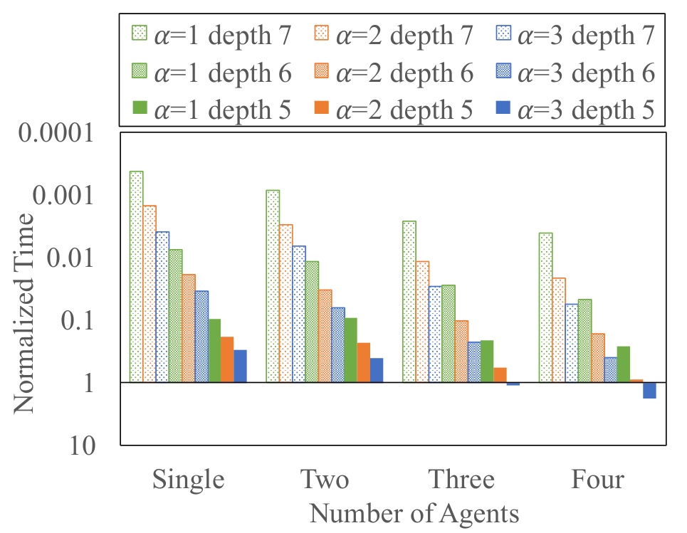
The computational advantage of the proposed algorithm is most prominent when the original search space is large and $\alpha$ is small (e.g., $\alpha=1$ depth 7), as the abstraction reduces the search space most significantly. The algorithm finds an abstract path three orders of magnitude faster compared to the regular A*. As we penalize the abstraction in the cost function defined in equation (2), the cost of the abstracted path is substantially worse compared to the resolution optimal solution especially for the single agent case. The increased number of agents improves the solution quality of the abstract path.

A similar comparison was made and plotted in Figure 6, but using instead the backtracking algorithm to solve for a fine resolution path. At each iteration, only one agent was allowed to move, while the other agents remained stationary. This was done to demonstrate the application of the algorithm for cooperative agents with different goal locations.

In the single agent case, the performance was highly sensitive to the choice of $\alpha$. At some abstraction structure, the single agent could still find near optimal solutions, but in the worst case, the path length was 16 times longer than the optimal. In contrast, as a better heuristic for refinement was used, the multi-agent cases resulted in more consistent computation times and cost performance that was less sensitive to the particular choice of $\alpha$.

In this paper, we propose a new algorithm to solve a single query shortest path planning problem using multiple multi-resolution graphs representing the same search space. The solution quality and the speeds up from abstraction is balanced efficiently by using multiple agents distributed in the search space, as they communicate only the expansion result of A* to avoid unnecessary communication. The completeness and optimality of the algorithm are shown. The proposed scheme was applied to a backtracking algorithm and demonstrated the advantages of using selective and distributed information provided by other agents for refinement heuristics in terms of computational time and solution quality.

This work has been supported by ARL under DCIST CRA W911NF-17-2-0181.

References

- [1] B. Marthi, S. Russell, and J. Wolfe, “Angelic hierarchical planning: optimal and online algorithms (revised).” University of California, Berkeley” Technical Report, 2009.
- [2] S. J. Kiebel, J. Daunizeau, and K. J. Friston, “A hierarchy of time-scales and the brain,” PLoS Computational Biology, vol. 4, no. 11, p. e1000209, 2008.
- [3] M. Helmert, P. Haslum, J. Hoffmann, and R. Nissim, “Merge-and-shrink abstraction: A method for generating lower bounds in factored state spaces,” Journal of the ACM, vol. 3, 05 2014.
- [4] S. Kambhampati and L. S. Davis., “Multiresolution path planning for mobile robots,” IEEE Journal of Robotics and Automation, pp. 135–145, 1986.
- [5] D. K. Pai and L. . Reissell, “Multiresolution rough terrain motion planning,” IEEE Transactions on Robotics and Automation, vol. 14, no. 1, pp. 19–33, Feb 1998.
- [6] R. Holte, M. Perez, R. Zimmer, and A. MacDonald, “Hierarchical A*: Searching abstraction hierarchies efficiently.” in AAAI, 1996, p. 530–535.
- [7] A. Botea, M. Müller, and J. Schaeffer, “Near optimal hierarchical path-finding,” Journal of Game Development, vol. 1, pp. 7–28, 2004.
- [8] H. A. Simon, “The architecture of complexity,” Proceedings of the American Philosophical Society, vol. 106, no. 6, pp. 467–482, 1962.
- [9] F. Hauer, A. Kundu, J. M. Rehg, and P. Tsiotras, “Multi-scale perception and path planning on probabilistic obstacle maps,” in IEEE International Conference on Robotics and Automation (ICRA), Seattle, WA, May 2015, pp. 4210–4215.
- [10] D. Jung, “Hierarchical path planning and control of a small fixed-wing uav: theory and experimental validation.” Ph.D. dissertation, Georgia Institute of Technology, Atlanta, GA, 2007.
- [11] R. V. Cowlagi and P. Tsiotras, “Multiresolution motion planning for autonomous agents via wavelet-based cell decompositions,” IEEE Transactions on Systems, Man, and Cybernetics, Part B (Cybernetics), vol. 42, no. 5, pp. 1455–1469, Oct 2012.
- [12] P. Tsiotras and E. Bakolas, “A hierarchical on-line path planning scheme using wavelets,” in 2007 European Control Conference (ECC), Kos, Greece, July 2007, pp. 2806–2812.
- [13] M. Otte and N. Correll, “C-FOREST: parallel shortest path planning with superlinear speedup,” IEEE Transactions on Robotics, vol. 29, no. 3, pp. 798–806, June 2013.
- [14] Y. Lu, Y. Huo, and P. Tsiotras, “A beamlet-based graph structure for path planning using multiscale information,” IEEE Transactions on Automatic Control, vol. 57, no. 5, pp. 1166–1178, May 2012.
- [15] R. Nissim and R. Brafman, “Distributed heuristic forward search for multi-agent planning,” Journal of Artificial Intelligence Research, vol. 51, no. 1, pp. 293–332, 2014.
- [16] P. E. Hart, N. J. Nilsson, and B. Raphael, “A formal basis for the heuristic determination of minimum cost paths,” IEEE Transactions on Systems Science and Cybernetics, vol. 4, no. 2, pp. 100–107, July 1968.