Dual parquet scheme for the two-dimensional Hubbard model:
Modelling low-energy physics of high- cuprates with high momentum resolution
Abstract
We present a new method to treat the two-dimensional (2D) Hubbard model for parameter regimes which are relevant for the physics of the high- superconducting cuprates. Unlike previous attempts to attack this problem, our new approach takes into account all fluctuations in different channels on equal footing and is able to treat reasonable large lattice sizes up to 32x32. This is achieved by the following three-step procedure: (i) We transform the original problem to a new representation (dual fermions) in which all purely local correlation effects from the dynamical mean field theory are already considered in the bare propagator and bare interaction of the new problem. (ii) The strong decay of the bare propagator allows us to integrate out all higher Matsubara frequencies besides the lowest using low order diagrams. The new effective action depends only on the two lowest Matsubara frequencies which allows us to, (iii) apply the two-particle self-consistent parquet formalism, which takes into account the competition between different low-energy bosonic modes in an unbiased way, on much finer momentum grids than usual. In this way, we were able to map out the phase diagram of the 2D Hubbard model as a function of temperature and doping. Consistently with the experimental evidence for hole-doped cuprates and previous dynamical cluster approximation calculations, we find an antiferromagnetic region at low-doping and a superconducting dome at higher doping. Our results also support the role of the van Hove singularity as an important ingredient for the high value of at optimal doping. At small doping, the destruction of antiferromagnetism is accompanied by an increase of charge fluctuations supporting the scenario of a phase separated state driven by quantum critical fluctuations.
pacs
71.27.+a, 71.10.FdI Introduction
Some of the features that make cuprates distinctly different from other known families of superconductors are the record high critical temperature at ambient pressure and the simultaneous presence of different collective modes in the phase diagram (for a review see, e.g., Refs. Damascelli et al. 2003; Vishik et al. 2010; Vishik 2018). At half-filling (i.e., in the undoped parent compound) and at low doping (), an antiferromagnetic (AFM) phase is observed. Strong spin fluctuations prevail in a much broader doping region ()Dagotto 1994, surrounding the narrow AFM state. This is not surprising taking into account the layered structure of cuprate compounds: in a purely planar system the AFM state would be fully suppressed at finite temperatureMermin and Wagner 1966 while the fluctuations would still be presentSchäfer et al. 2015. However, it can be disputed how the AFM state breaks down at the microscopic level. Several scenarios have been proposed including the formation of spin and charge stripesVojta 2009; Fujita et al. 2012, a phase separated state where extra charges form dropletsStepanov et al. 2018 in the AFM medium and even glassy phasesSeibold et al. 2014. On the single-electron level, a destruction of the AFM ordering is accompanied by the formation of the famous pseudogap state Yoshida et al. 2006, in which the Fermi surface near the anti-nodal direction is destroyed, likely because of the strong collective fluctuations.Gunnarsson et al. 2015
A further increase of doping away from half-filling results in the formation of the superconducting (SC) state with d-wave symmetry.Wollman et al. 1993; Shen et al. 1993 In the (temperature vs. doping) phase diagram, it forms a dome peaked at optimal doping . While this feature is virtually common to all hole-doped cuprate compounds, the nature of the superconducting phase is, however, still highly debated. The absence of an isotope effectPringle et al. 2000; Greco and Zeyher 2015 of the form suggests that the pairing glue for the electrons is not (exclusively) due to phonons. Instead, collective excitations of the electrons themselves, such as the above mentioned antiferromagnetic spin fluctuations, may generateSchmalian et al. 1998; Scalapino 2012 an effective attractive interaction. As an additional ingredient which is potentially responsible for the high value of at optimal doping the presence of a van Hove singularity has been discussed.Markiewicz 1997; Piriou et al. 2011
The above mentioned formation of a pseudgap as well as the anomalous non-Fermi-liquid-like behavior of certain transport properties with doping and temperatureLegros et al. 2019; Jenkins et al. 2010 indicate that the physics of the cuprates originates from –or is at least substantially affected by– strong correlation effects between the electronsLee et al. 2006. This is consistent with the widely accepted assumption that the physical properties of cuprates are dominated by the electrons in the partially filled orbital of the copper atoms in the CuO2 planes. Therefore, the planar single-band Hubbard modelHubbard 1964 on a square lattice, which incorporates correlation effects via a purely local on-site Coulomb repulsion , is commonly used for the theoretical description of these compounds. One should mention, that this model neglects several possibly important degrees of freedom in realistic cuprate crystals: The tunnel coupling between different CuO2 planes, phonon degrees of freedom which may be responsible for the experimentally observed charge density wavesReznik et al. 2006; Greco and Zeyher 2015; Miao et al. 2017, or oxygen -orbitals which can give rise to a metal-to-insulator transition of charge-transfer type.Avella et al. 2013; Hansmann et al. 2014 Nevertheless, the Hubbard model is usually considered as a minimal model which incorporates the important correlations effects in the Cu orbitals.Anderson 2002
Thus, mapping out the phase diagram of the Hubbard model is vitally important for our understanding of the physics of cuprates. Calculations for the Hubbard model are, however, extremely difficult in the parameter regimes relevant to cuprate systems. Although, the d-wave superconductivity arises in both the strong and the weak coupling limit of the Hubbard Hamiltonian, in the cuprates the value of the Coulomb interaction is comparable to the bandwidth (). This prevents any perturbative treatment in both and starting from the weakly interacting Fermi gas or isolated atoms, respectively. The sign problemLoh et al. 1990, on the other hand, imposes severe difficulties for lattice Quantum Monte Carlo calculations away from half-filling. Embedding approaches such as the density matrix embedding theoryKnizia and Chan 2012 or the site occupation embedding theorySenjean 2019 are restricted to zero (or very low) temperature and/or to one-dimensional systems. Similar problems arise for the density matrix renormalization group techniqueHallberg 2006 which provides almost exact results in one dimension but is very hard to extend to higher dimensions. A recently suggested numerical renormalization group methodHuang et al. 2018 is confined to zero temperature and small lattice sizes ( stripes). Functional renormalization group (fRG) approachesHalboth and Metzner 2000; Metzner et al. 2012 are a powerful tool to take into account the mutual screening between competing bosonic modes. However, they can provide an accurate quantitative description only at weak coupling.
To overcome the above-mentioned difficulties, a comprehensive theory for the solution of the 2D Hubbard model should be able to correctly capture at least the two most important features of this system: (i) It should incorporate nonperturbatively strong local correlation effects leading to the spectral weight-transfer and renormalization of the electronic density of states, and (ii) it has to take into account long-range correlation effects due to competing collective bosonic modes in different scattering channels. The situation becomes even more complicated because these phenomena occur at very different energy scales ranging from meV [for (ii)] to several eV [for (i)].
As for local correlations, the dynamical mean field theory (DMFT) Metzner and Vollhardt 1989; Georges and Krauth 1992; Georges et al. 1996 has become the standard tool for the description of correlated model systems and materials by replacing the actual lattice of interacting sites by a single interacting site embedded in a self-consistent noninteracting bath. In this way, DMFT takes into account all purely local correlations but captures long-range bosonic collective modes only on a mean-field level. In particular, the mutual interaction and screening effects between bosonic fluctuations in competing channels are not sufficiently considered.
The most straightforward way to overcome this problem and include spatial nonlocality in the framework of DMFT is to use cluster methods instead of the single-site scheme. This has lead to the development of the cellular DMFT (CDMFT) and the dynamical cluster approximation (DCA) which consider a cluster of interacting site in real or momentum space, respectively. CDMFT calculations with a properly periodized 22 cluster indeed yield a SC phaseLichtenstein and Katsnelson 2000; Maier et al. 2005. DCA approaches Yang et al. 2011; Chen et al. 2013; Gull et al. 2013; Chen et al. 2015 applied to larger clusters have been able to capture antiferromagnetic spin fluctuations and a dome-like SC phase with quite close to the experiment. Several important physical conclusions have been drawn from the DCA results. In particular, they are consistentKhatami et al. 2010; Yang et al. 2011 with the scenario of a quantum critical point (QCP) Varma 1999; Broun 2008; Sachdev 2010 underlying the SC area in phase diagram and moreover predict various phenomena such as phase separationKhatami et al. 2010, a Lifshitz transitionChen et al. 2012, a momentum-sector-selective metal-insulator transitionGull et al. 2009 or pseudogap behaviorGunnarsson et al. 2015; Gunnarsson et al. 2016; Gunnarsson et al. 2017 .
Unfortunately, cluster approaches can take into account nonlocal correlations only within the cluster size. This is limited by the exponential growth of the Hilbert space to about sites even within a single orbital model. Phenomena such as a QCP or spin fluctuations are, however, intrinsically long-ranged. Convergence of the results with the cluster size can be therefore be questioned. To circumvent such problems, diagrammatic extensionsRohringer et al. 2018 of DMFT have been suggested in the last decade. They allow, at least in principle, to handle correlations at all length and energy scales on equal footing. These approaches construct a perturbation theory around DMFT using the Green’s function and the local two-particle vertices of DMFT as building block for the diagrammatic expansions. These schemes benefit from a natural separation of high-energy local physics, which is accounted for by DMFT, and the low-energy bosonic collectve modes, which are treated diagrammatically. Various flavors of diagrammatic extensions of DMFT have been developed, such as the dynamical vertex approximation (DA)Toschi et al. 2007, the dual fermion (DF)Rubtsov et al. 2008 theory, the dual boson (DB)Rubtsov et al. 2012 scheme, the one-particle irreducible approach (1PI)Rohringer et al. 2013, the TRILEXAyral and Parcollet 2015; Ayral and Parcollet 2016a, and the QUADRILEXAyral and Parcollet 2016b method, as well as mergers of (extended) DMFT and fRG such as the DMF2RGTaranto et al. 2014 and the 2PI-fRGKatanin 2019 approaches. They differ mainly in the choice of diagrams which are constructed on top of DMFT. In most cases, random phase approximation (RPA)Mahan 2000- or fluctuation exchange (FLEX)Bickers and Scalapino 1989-like diagrams in one scattering channel have been considered. This, however, requires an a priori knowledge of the dominating fluctuations and cannot describe the interplay between different channels which is necessary to obtain -wave superconductivty from the repulsive Hubbard model. Multichannel FLEX diagramsBickers 2004, on the other hand, indeed predict d-wave superconductivity. However, different flavors of diagrammatic extension of DMFT that use such diagrams yield very different phase diagrams, showing rather poor coincidence with the experimentally observed one. For example, TRILEX produces the superconducting dome, but not the AF peak. FLEX-like diagrams with DFOtsuki et al. 2014, which consider the particle-hole and particle-particle channel, can describe antiferromagnetism well and give rise to the superconductivity, but they do not show the SC-dome structure. FLEX+DMFT calculationsKitatani et al. 2015, on the other hand, produce a far too broad dome. The DA-ladder calculation of the pairing vertex does indicate a dome which is, however, located at very small doping when a realistic electron dispersion is considered.Kitatani et al. 2019 Overall, multichannel FLEX-like diagrams suffer from the insufficient treatment of the mutual screening between competing fluctuations.
A quantitatively accurate theory which takes into account all mutual screening effects between the different bosonic modes and is self-consistent at the one- and the two-particle level can be built from the parquet equationsDiatlov et al. 1957; Bickers 2004. They construct all one- and two-particle correlation functions from the fully irreducible vertexRohringer et al. 2012 of the system. Approximating this vertex with the bare interaction leads to the so-called parquet approximationYang et al. 2009; Tam et al. 2013. In the framework of diagrammatic extension of DMFT, the DA replaces the fully irreducible vertex by the corresponding local one of DMFTLi et al. 2016. However, although the method formally obeys a polynomial complexity, in practice it is numerically very expensive as it requires the full two-particle vertex functions which depend on three frequencies and three momenta. This restricts practical calculation to very small momentum grids of about 6x6 sites, even if one uses highly elaborated parametrizations of the frequencyKarrasch et al. 2008; Wentzell et al. 2016; Tagliavini et al. 2017 and the momentumEckhardt et al. 2018 grids or solves the parquet equations by means of the multiloop fRGKugler and von Delft 2018a; Kugler and von Delft 2018b technique.
To mitigate these limitations, we propose a parquet method in which the Matsubara frequency grid is reduced to the lowest Matsubara frequencies. Our method can be presented as a three-step procedure: First, we solve the local DMFT impurity problem which provides us the basic elements for our diagrammatic expansion, i.e., the DMFT Green’s function as well as the local vertex function. Secondly, we integrate out the higher Matsubara frequencies using the dual-fermion theory which provides an optimal framework for a diagrammatic expansion around DMFT. Third, we solve our low-frequency effective model by means of the parquet equations which is possible due to the reduction to only a few Matsubara frequencies for lattices up to 32x32 sites.
The plan of the paper is the following: In Sec. II we present the basic formalism and derive our method. Our results for the 2D Hubbard model are discussed and compared to other approaches in Sec. III. Specifically we plot the phase diagram, calculate the fluctuations in spin, charge and superconducting channels for different points of the high-temperature phase, and analyze the pairing glue and the origin of the dome structure observed in our study. Sec. IV is devoted to conclusions and an outlook.
II Model and method
II.1 Definition of the model and DMFT
We consider the Hubbard Hamlitonian on a 2D square lattice:
| (1) |
where is an annihilation (creation) operator for an electron with momentum (or at lattice site ) and spin . . The dispersion relation is given by , is the chemical potential, and denotes the Coulomb repulsion between two particles at the same lattice site.
Within the DMFT approximation, one replaces the actual lattice of interacting sites by a single interacting site (=impurity) which hybridizes with a noninteracting bath. This corresponds to an Anderson impurity model (AIM) which can be represented by the action
| (2) |
where are the Grassmann fields corresponding to the operators , is an imaginary time, , , the corresponding fermionic Matsubara frequency, and the inverse temperature. Summations over Matsubara frequencies include the normalization factor . The hybridization function between the impurity and the bath is determined by the DMFT self-consistency condition which requires the local part of the lattice Green’s function in the DMFT approximation (i.e., with the self-energy replaced by the local one of the impurity problem) to be identical to the corresponding impurity Green’s function:
| (3) |
where is the local impurity self-energy and the impurity Green’s function. The is the normalized momentum integral over the first Brilluoin zone (BZ) with the volume . The impurity self-energy captures all purely local correlations of the system while nonlocal correlations are neglected. In the next section, we will outline our new approach which constructs nonlocal correlations from the DMFT starting point.
II.2 Low-frequency model and parquet equations
Our new approach to find an (approximate) solution of the Hubbard model can be divided into three steps which we outline in the following.
II.2.1 Local correlations and DF transformation
Since an exact calculation of the one- and two-particle correlation functions for the Hamiltonian in Eq. (1) is not possible so far we have to apply perturbation theory. However, a perturbative expansion in the bare Green’s function and the bare interaction cannot capture the important local correlations and the related MottMott 1968 physics. Hence, a reformulation of perturbation theory in terms of the DMFT Green’s function and the local DMFT two-particle vertex [i.e., the vertex of the AIM Eq. (II.1)] is highly desirable. In this way, all purely local correlations are included already in the building blocks of a Feynman diagrammatic expansion while the latter itself will add nonlocal correlation effects which are absent in DMFT.
The DF theoryRubtsov et al. 2009 provides a convenient formal framework for the construction of a diagrammatic perturbation theory around DMFT. In this approach, the action of the Hubbard Hamiltonian Eq. (1) is separated into a local impurity part and a remainder
| (4) |
To obtain an effective perturbation theory around the local DMFT physics, we separate local and nonlocal degrees of freedom by decoupling the second term on the right-hand side of Eq. (4) via a Hubbard-Stratonovich transformationHubbard 1959; Stratonovich 1957 (for the explicit procedure see, e.g., Ref. Rohringer et al. 2018). The corresponding Hubbard Stratonovich fields and are typically labelled “dual fermions”. One can now integrate out the original fields and to obtain the action of the Hubbard model in terms of the dual particles
| (5) |
where is the bare dual propagator which is given by the difference between the full momentum dependent and the local DMFT Green’s function and, hence, accounts for the nonlocal degrees of freedom. The effective interaction between the dual fermions is given by local two-, three-, particle vertices of the AIM. While the role of three- and more-particle terms has not been fully clarified so farRohringer et al. 2013; Ribic et al. 2017, a truncation at the two-particle level is a reasonable approximation considering that the original Hubbard interaction is of two-body type. With this approximation the effective interaction between the dual fermions becomes
| (6) |
where denotes the local two-particle vertex of the AIM and , , is a bosonic Matsubara frequency.
II.2.2 Effective low-frequency model
The complex frequency dependence of the effective interaction makes a diagrammatic expansion for the action in Eq. (5) very difficult. In particular, the dependence of the vertex on three frequencies typically restricts the choice of Feynman diagrams to rather simple topologies such as ladders in a single scattering channel. Since this is not sufficient for the description of competing fluctuations, a simplification of the frequency and/or momentum dependence of the one- and two-particle correlation functions is highly desirable.
The second step, and at the same time central idea, of our new approach is a reduction of complexity in the frequency domain in the dual action Eq. (5). To achieve this, we split the -variable in the spirit of Wilson’s renormalization groupWilson 1975 into a low- and a high-energy part
| (7) |
where is the cutoff frequency.
This allows us to separate the total action in Eq. (5) into a lesser part which depends only on and a greater part which depends on both and :
| (8) |
Then, we integrate out high-frequency fields in the functional integral representation of the partition function considering the diagrams depicted in Fig. 1 for the perturbative expansion of :
| (9) |
which gives rise to the effective low-frequency action
| (10) |
where denotes an expectation value with respect to the high-frequency fields, i.e., taking the path integral over all fields and with . The resulting action depends only on the lowest fermionic Matsubara frequencies . To present the explicit expression, we use a simplified notation adopting a multi-index which includes frequency, momentum, and spin degrees of freedom. In this notation, the effective action reads
| (11) |
where the effective bare propagator is given by
| (12) |
and the effective bare interaction can be represented as
| (13) |
where a summation/integration over repeated indices is assumed.
Let us stress, that similar simplifications of the frequency dependence of the vertex function has been used also for fRG studies of the 2D Hubbard modelHonerkamp and Salmhofer 2003; Metzner et al. 2012. However, these approaches differ in two crucial aspects from our approach.
(i) First, and probably most important, in the above-mentioned fRG studies the simplification in the frequency domain has been applied directly to the Hubbard model in Eqs. (1). In this case, the bare propagator for the construction of a diagrammatic perturbation theory decays as for . On the contrary, starting from the dual action in Eq. (5), the bare propagator decays much faster, i.e., as , which supports the general picture of the DF approach as a theory, which constructs low-energy (or low-frequency) corrections around the DMFT solution of the Hubbard model.
(ii) The second difference between our new technique and the above-mentioned fRG schemes is that in the latter approaches the frequency space has just been truncated to the lowest Matsubara frequency, losing information about the effect of the high-energy onto the low-energy physics. In our approach, this information from higher frequencies is partially taken into account by our downfolding procedure. This may be particularly important in the presence of strong correlations where the formation of Hubbard subbands occurs at such high frequencies. The overall importance of the downfolding procedure and the question whether the diagrams in Fig. 1 are indeed sufficient for a comprehensive description of the effective model requires, however, further inverstigation.
II.2.3 Parquet equations
The simplifications leading to in the previous section allow us now to apply highly advanced diagrammatic techniques for the treatment of our effective problem. The parquet formalism is an approach, which is able to take into account fluctuations in all scattering channels (i.e., spin, charge, and particle-particle or pairing channel) as well as their mutual interaction and screening effects. It constructs the full two-particle vertex function from a single input quantity, i.e., the fully irreducible vertex function . Moreover, the one-particle self-energy is derived from the full vertex via the equation of motion which guarantees the consistency between the one- and the two-particle correlation functions.
For completeness, let us briefly recapitulate the parquet formalism (for details we refer to Appendix C and Refs. Rohringer et al. 2012; Rohringer et al. 2018): The full vertex can be decomposed into a fully irreducible vertex and vertices reducible in particle-hole, particle-hole transverse and particle-particle channels (). This decomposition is expressed by the purely algebraic Parquet equation
| (14) |
which is represented diagrammatically in Fig. 2. The reducible vertices , in turn, correspond to ladder diagrams in the given scattering channel which are constructed from the corresponding irreducible vertex as (where denotes the single-particle Green’s function). This gives rise to the so-called Bethe-Salpeter (BS) equations in all three scattering channels , , and .
| (15a) | ||||
| (15b) | ||||
| (15c) | ||||
which are depicted diagrammatically in Fig. 2. Let us stress that, in contrast to the simple algebraic parquet Eq. (14), the BS Eqs. (15a) are complex integral equations since a summation over the repeated indices 5,6,7, and 8 has to be performed. For a fixed input , Eqs. (14) and (15a) are iterated for a given one-particle Green’s function (see small inner loop on the right-hand side of the flow diagram in Fig. (5). After convergence, a new self-energy is obtained from via the so-called Schwinger-Dyson equation (or Heisenberg equation of motion)
| (16) |
which is depicted diagrammatically in Fig. 4. From the updated , a new Green’s function is obtained through the Dyson equation which is used, in turn, to reiterate the vertex functions (see large outer loop in the flow diagram in Fig. 5).
Since the fully irreducible vertex of a system is in general not known, approximations for this quantity have to be applied. The most simple one, the so-called parquet approximationBickers 2004, replaces the fully irreducible vertex simply by the bare interaction. Applying this procedure directly to the Hubbard model in Eq. 1, leads to a theory which is applicable only at weak coupling. Moreover, a truncation to only the lowest Matsubara is less justified for the same reasons as discussed at the end of Sec. II.2.2. On the contrary, the bare interaction of our effective theory has inherited the local strong coupling Mott physics from DMFT, so that the high-energy physics is taken into account while changing to the new variables. Hence, the choice and working with lowest Matsubaras only should yield reasonable results at strong coupling and, at the same time, captures the physics of competing bosonic fluctuations via the ladder and parquet diagrams of the parquet formalism. Let us again stress, that due to the simplified frequency structure of our theory, the parquet equations can be solved on a much finer momentum grid than in previous parquet calculationsLi et al. 2017.
II.3 Technical details
We solve the impurity problem using an Exact Diagonalization solver and compute local Green’s functions and local two-particle vertex functions for a given temperature and chemical potential. The Parquet solver extensively uses CUDA for parallel computations.
As discussed in the previous section, the Parquet formalism involves the iteration of an inner and an outer self-consistency loop for the vertex function and the self-energy , respectively (see Fig. 5). The initial guess of and is essential for the convergence of the algorithm to a stable solution. The most convenient way for the initial guess is to choose all irreducible vertices and the full vertex equal to , and put an imaginary part of the self-energy equal to a very large number (several bandwidths) in order to sufficiently suppress the size of the ladders in the BS equation in the first iteration. To avoid instabilities, damping factors for updates have been introduced:
| (17a) | ||||
| (17b) | ||||
We have also enforced conservation of crossing symmetry during the calculationsTam et al. 2013.
The main advantage of the Parquet formalism with respect to cluster calculations is that it scales algebraically with the size of the system (, where is a number of spin components) in contrast to the exponential scaling of cluster methods. Let us emphasize that in our case a further reduction of complexity is achieved by .
III Results
In this section, we present the results for the 2D Hubbard model on a square lattice as obtained by the approach discussed in the previous Sec. II. For the nearest-, next-nearest- and next-next-nearest-neighbor hopping parameters we have selected the values eV, and , respectively, which are relevant for the high-temperature superconducting cuprate compound BSSCONicoletti et al. 2010. The interaction value has been chosen as which corresponds to an intermediate-to-strong coupling regime for which at half-filling a Mott metal-to-insulator transition is observed in DMFTGeorges et al. 1996. For the solution of the parquet equations we have discretized the Brillouin zone using -points in each direction for most of the calculations and -points in specific situations in order to analyze the dependence on the grid size.
The calculations have been performed at different values of the chemical potential . The corresponding number of particles per lattice site or, correspondingly, the doping have been calculated in the standard way by summing the one-particle Green’s function over frequencies and momenta, i.e., with . For the lowest Matsubara frequency , the one-particle Green’s function of our downfolded model has been obtained by means of the parquet equations, while for the larger frequencies the Green’s function of DMFT has been used for the calculation. This procedure is justified by the fact, that nonlocal correlations (or correlations in general) affect most strongly the low-energy physics while at higher frequencies the Green’s function approaches its non-interacting value. However, it should be mentioned that a rigorous verification of this assumption requires a systematic extension of the effective low-frequency model to two and more Matsubara frequencies, which will be considered in a future research work (see outlook in Sec. IV). In any case, while close to half-filling and at very low temperatures the dependence of on can exhibit a rather complicated singular behaviorNourafkan et al. 2019, Fig.6 shows that for higher values of considered here, is a regular featureless function which does not differ much from the curve obtained using DMFT. For lower values of temperature however the difference is increased but still stays regular and relatively small near the optimal doping. This has allowed us to straightforwardly recast our results in the following sections, which have been originally obtained for fixed values of , in terms of the filling (or, equivalently, of the doping ).
III.1 Phase diagram

Fig. 7 shows the phase diagram of the Hubbard model as a function of temperature and doping. Close to half-filling (), we observe an antiferromagnetic phase with a quasi-long-range order while at larger values of the doping a superconducting phase emerges.
The notion of “phase” in the present context should be clarified. Let us stress that here it does not refer to a state with a real long-range order in the thermodynamics limit which would be signaled by a diverging spin or pairing susceptibility at the transition point. In fact, in 2D a long-range magnetic order is restricted to according to the Mermin Wagner theoremMermin and Wagner 1966. On the other hand, a superconducting state of Kosterlitz-Thouless type can exist in 2D at finite temperatures, characterized by a diverging correlation length but a finite susceptibilityKosterlitz and Thouless 1973 which can, however, not be accessed by our method.
Instead, the colored regions in Fig. 7, which mark the different phases, indicate the areas where the corresponding antiferromagnetic or superconducting fluctuations become very large which is reflected in a sizable magnitude of the corresponding susceptibilities or vertex functions . These correlation functions are obtained from the Bethe Salpeter equation
| (18) |
in the spin () and pairing () [and, in the next section, charge (] channels, respectively. Here, we have used a condensed notation where [] corresponds to a composite index for a fermionic [bosonic] Matsubara frequency and a momentum vector (for the exact definition of all vertex functions and channel indices we refer to the Appendix). For a given irreducible vertex , Eq. (18) represents a matrix equation in the space for the calculations of . Since the evaluation of requires the inversion of the operator , it is obvious that strongly increases when the largest (leading) eigenvalue of the kernel approaches :
| (19) |
where denotes the corresponding eigenvector. In this section, we are interested in antiferromagnetic spin and pairing instabilities which are related to the eigenvalues and . The values of and have been determined for various fillings starting from the high-temperature unordered state. We have then gradually decreased the temperature until one of the eigenvalues reached a value close to one indicating the proximity of the corresponding instability. Let us note that for each value of the temperature, we had to perform a series of calculations with fixed chemical potential until the desired filling (or doping ) was found.
Following the described strategy, we can identify an antiferromagnetic region (red shaded area) at small doping in Fig. 7 whose border (black crosses in Fig. 7) is defined by the corresponding antiferromagnetic eigenvalue of approaching a value of upon lowering the temperature. A further decrease in temperature (for a given doping) allows us to find an eigenvalue of even closer to one (black dot in Fig. 7). For larger values of , we observe an increase of the superconducting eigenvalue defining the border of the superconducting region of the phase diagram (blue shaded area). Interestingly, the difference between the temperatures at which (blue crosses) and (blue dots) is much smaller than for the antiferromagnetic case where K at . This indicates that strong superconducting fluctuations are restricted to a small area of the phase diagram around the superconducting dome while the AF fluctuations seem to be sizable in a larger region of the phase diagram. This finding is also consistent with the Mermin Wagner theorem which predicts the ordered state only at while rather large AF fluctuations extend to a wide region of the phase diagram.
III.2 Leading eigenvalues
In order to obtain further insights into the nature of the different phases and their related fluctuations, we present here a more detailed analysis of the leading eigenvalues for the antiferromagnetic spin (), the superconducting () and the uniform charge () channel in Figs. 8-10.
Figure 8 shows and as a function of the temperature at optimal doping where the superconducting dome reaches its maximum. The antiferromagnetic eigenvalue is considerable in a broad temperature range and increases slightly only at the lowest temperature. The superconducting eigenvalue , on the other hand, is almost at higher temperatures and increases rapidly only at temperatures very close to the superconducting dome where it crosses and eventually becomes larger than . At the lower value of the doping (), the superconducting fluctuations are strongly suppressed over the entire accessible temperature range as it can be seen in Fig. 9. As expected, the antiferromagnetic fluctuations are larger close to half-filling and increase upon lowering the temperature. Finally, let us analyze the leading eigenvalues as a function of doping at the maximum temperature of the superconducting dome (see Fig. 10). As expected, for lower values of antiferromagnetic fluctuations dominate while is almost zero. Upon increasing doping one approaches the superconducting dome which is reflected in a strong increase of which eventually crosses the leading antiferromagnetic eigenvalue. The latter exhibits a much weaker doping dependence and is sizable also in the region where approaches . We can, hence, conclude that antiferromagnetic fluctuations are relevant in the entire phase diagram with an expected maximum at low values of doping and temperatures while superconducting fluctuation are sharply restricted to a region very close to the superconducting dome. This also agrees with the fact that antiferromagnetic fluctuations provide the effective “pairing glue” for the electrons in order to form a superconducting state and, hence, should not be small close to the superconducting area of the phase diagram.

Let us discuss the role of uniform [] charge fluctuations which are reflected by the behavior of the corresponding eigenvalue . As expected for a system with a repulsion between the particles, charge fluctuations are suppressed in a large region of the phase diagram. In particular, close to half-filling ( in Fig.9) is almost 0 for all temperatures with a small increase for . Interestingly, at optimal doping (Fig. 8) this increase upon lowering is much more pronounced which indicates that in the region where -wave superconductivity prevails also charge fluctuations become non-negligible. Turning our attention to the doping dependence of in Fig. 10, we observe a very interesting feature: For the maximal superconducting temperature , exhibits a maximum at . One can speculate that this remarkable behavior might be a signature of a quantum critical point triggered by charge fluctuations which is responsible for the physics observed in a wide range of the phase diagram although it has to be said that such features are typically found at larger values of doping in DCA calculations.Yang et al. 2011. Moreover, enhanced charge fluctuations support the picture that AF order breaks down due to the formation of a phase separated stateKhatami et al. 2010 in which the holes form (maybe virtually) droplets in the AF background as predicted in Ref. Stepanov et al. 2018. While in the latter paper only nonlocal fluctuations in the spin channel were taken into account, our dual parquet calculations allow to access the charge channel also, and the emergence of an increased charge susceptibility at indeed provides a new and solid argument in favor of the phase separation picture. We note however that our results cannot exclude other scenarios for the breakdown of antiferromagnetism, such as striped phase (see Sec. III.3) for a different choice of the model parameters, in particular the value of .
Let us finally comment on the dependence of the results on the number of -points in the Brillouin zone used for the calculations. While the AF fluctuations exhibit a rather strong dependence on the momentum gridSchäfer et al. 2015 due to the exponentially large correlation length at low values of , the difference between and -points (see orange dot in Fig. 7) for the definition of the superconducting region at optimal doping is very small, which indicates the stability of the superconducting dome w.r.t. to larger momentum grids.
III.3 Type of superconducting and spin fluctuations

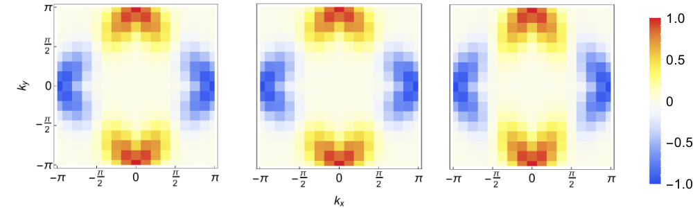

In this section, we investigate the type of the magnetic and superconducting fluctuations which we have identified in the previous sections. To this end we analyze the momentum dependence of the corresponding susceptibilities and eigenvectors of the BS kernels which are related to the leading eigenvalues [see Eq. (19)].
An evaluation of the physical susceptibility requires the summation of the generalized susceptibility
| (20) |
over the fermionic indices and (i.e., over the fermionic Matsubara frequencies and as well as over the momenta and ):
| (21) |
For the evaluation of this expression we consider only the two lowest Fermionic Matsubara frequencies for the summation over the fermionic indices, because only are present in our downfolded effective action.
One could think about a more sophisticated solution in analogy to the above calculation of , where we have adopted the DMFT Green’s function for the summation over the higher frequencies (see the discussion at the beginning of Sec. III). However, using the DMFT results for the two-particle quantity for in Eq. (21) is questionable as the DMFT susceptibilities are obtained from a single Bethe-Salpeter equation in the given channel neglecting mutual screening effects between the channels. Hence, such a construction might add a bias to the (channel-unbiased) parquet results for the low-frequency model and, hence, worsens the results. Moreover, it is currently unclear how to treat the situation where and (or vice versa) which would require a deeper analysis of this problem by tracing the calculation of the generalized susceptibilities within the downfolding procedure. In general we expect, that the above described calculation of susceptibilities, using only the lowest fermionic Matsubara frequencies, yields reasonable results because long-range bosonic fluctuations are typically assiciated with low energies. Nevertheless, the problem of a consistent evaluation of within our low-frequency model requires further investigation.
Figure 11 shows the spin susceptibility for the bosonic frequency as a function of and . Consistent with the analysis of the eigenvalues, at low doping antiferromagnetic spin fluctuations dominate which is indicated by a strong peak at . For larger dopings, this maximum of is reduced but, nevertheless, remains at the wave vector . This proves that the spin fluctuations, which have been shown to be sizable in the entire phase diagram, are indeed of antiferromagnetic nature in the whole parameter regime under investigation. This is also consistent with the results obtained earlier by DCA in Ref. Chen et al. 2013. In particular, our data preclude the emergence of spin stripes which have been discussed controversially on both the experimentalFujita et al. 2012; Tranquada 2012 and the theoreticalVojta 2009 side. This further strengthens the assumption that antiferromagnetism break down due to the formation of a phase separated state rather than due to a stripe ordered state as discussed at the end of Sec. III.2.
Let us now turn our attention to the pairing fluctuations. As expected, close to a superconducting instability, is strongly peaked at close to the superconducting dome. This feature is well reproduced by our numerical data in Fig. 12 which also gives further support for the validity of our approximation for the calculation of . The physically more interesting question, however, concerns the nature of the superconducting fluctuations. Such an information is encoded in the momentum dependence of the eigenvectors [see Eq. (19)] of the BS equation which corresponds to the leading superconducting eigenvalue. In Fig. 13 these eigenfunctions are shown for three different values of the doping at temperatures close to the superconducting dome (i.e., where the corresponding leading eigenvalue is ). One observes a clear -wave structure corresponding to an eigenfunction for all values of the doping. In order to quantify this qualitative finding we have projected onto the -, - and -wave form factors [, or and ], respectively. This results in a fraction of 0.86, 0.92 and 0.85 for the -wave, 0.04, 0.03 and 0.05 for the -wave and 0.1, 0.05 and 0.1 for the -wave contribution for , 0.15 and 0.19, respectively. These numerical results, hence, clearly reflect the -wave nature of the superconducting fluctuations. Let us stress that our results for the susceptibilities are stable with respect to the size of the momentum grid as it is illustrated in Fig. 14 for a 32x32 -lattice.
III.4 Pairing glue and origin of the dome structure
An important question regarding the phase diagram of the 2D Hubbard model concerns the origin of the pairing glue and -related to this problem- the reason for the dome-like structure of the superconducting region. To this end, we analyze the BS equation for the generalized susceptibility in the (singlet) pairing channel
| (22) |
where is the bare pairing bubble and two-particle irreducible vertex in the singlet pairing channel. Considering the relation between and in Eq. (III.3), Eq. (22) corresponds one-to-one to the BS equation for discussed in Sec. III.1 and, hence, an eigenvalue indicates a divergence of [i.e., a vanishing of the l.h.s. of Eq. (22)]. Obviously, a zero on the l.h.s. of Eq. (22) has to be generated by the interplay between the bare pairing susceptibility and the irreducible (singlet) pairing vertex which represents the effective attractive interaction between the electrons. Unfortunately, such an interplay is difficult to analyze because the objects in Eq. (22) are matrices in the fermionic (frequency and momentum) variables and . In order to get a better physical intuition we follow the ideas11 1 Note that, differently from Ref. Yang et al. 2011; Chen et al. 2013 we have projected instead of as this allows for a direct projection of the BS equation (22). of Ref. Chen et al. 2013 and average all quantities over the fermionic indices and whereas for the momentum average we include the -wave form factor :
| (23a) | ||||
| (23b) | ||||
Applying this projection to Eq. (22) we obtain a Stoner-like criterion for the vanishing of the projected inverse susceptibility :
| (24) |
where can be interpreted as effective pairing interaction. In Fig. 15 we have plotted and at the maximal temperature of the superconducting dome as a function of doping. A touching of the two curves corresponds to the onset of superconducting order. One can clearly see that neither nor exhibit a dome structure as a function of doping which, hence, originates from an interplay of these two quantities. Remarkably, (blue line) exhibits a monotonous increase of the effective pairing interaction upon lowering the doping and takes it maximum at half-filling where antiferromagnetic spin fluctuations dominate. In order to gain a better physical understanding of this interesting behavior of , we use the parquet equation
| (25) |
and project it on the -wave form factor as in Eqs. (23). In this way, can be split into three contributions , and originating from the fully irreducible vertex , form the reducible charge vertex and from the reducible spin vertex , respectively. Fig. 16 shows that the major contribution to the -wave pairing glue can be traced back to spin fluctuations represented by (i.e., the -wave projection of the reducible spin vertex, red line). A further examination of the momentum sum for the calculation of [see also Eqs. (23)] reveals that the by far most important contribution stems from a single grid point (orange curve) which confirms that antiferromagnetic spin fluctuations can be identified as the main source for the pairing glue which leads to superconductivity in the model.
The same antiferromagnetic fluctuations which make large, on the other hand, open a gap in the spectral function and, hence, suppress the one particle Green’s function and consequently the bubble . This triggers a corresponding increase of upon lowering the doping (black line), leading to the above mentioned competition between this quantity and which is responsible for the dome structure of the superconducting phase.
Let us finally mention an interesting feature observed in at optimal doping (, where the curves touch each other. There, shows a non-monotonous behavior and exhibits a minimum as a function of doping. This feature can be seen as an increase of the effective density of states (DOS) near the Fermi level and appears, hence, to be responsible for the strong enhancement of superconducting fluctuations while is monotonous and rather featureless in this region of the phase diagram. In Fig. 15, we have also plotted the DMFT data for (thin black line). It can be seen that the DMFT also shows a peculiarity in , although it is less pronounced and slightly shifted to the smaller doping.
The increase in the DOS can be attributed to the effect of a van Hove singularity, which crosses the Fermi level close to optimal doping. In correlated systems, the corresponding flattening of the dispersion law has to be attributedDzyaloshinskii 1996; Irkhin et al. 2001 to non-Fermi liquid effects. They enhance the contribution of van Hove singularities to the DOS with respect to the expression known for the noninteracting Fermi gas in 2D. This enhancement is not seen on the DMFT level (see thin black line in Fig. 15) but arises in nonlocal extensions of DMFTRubtsov et al. 2009. Whether the observed behavior is related to the anomalous temperature behavior of the the bubble , which has been reported in DCA studiesYang et al. 2011; Chen et al. 2012 and related to a quantum critical point below the superconducting dome, is a question for future research work.
III.5 Spectral properties
Let us turn our attention to spectral properties obtained from our parquet equations. Since the self-energy and the Green’s function are known only for the first fermionic Matsubara frequencies it is difficult to perform an analytic continuation to the real frequency axis in order to obtain a spectral function. However, interesting information can be already extracted from the self-energy at the lowest Matsubara frequency. Fig. 17 shows for as a function of and . Our results confirm the general wisdom that in the underdoped regime of the 2D Hubbard model above the superconducting dome a pseudogap region emerges with a momentum selective suppression of spectral weightGull et al. 2009. Our data indeed show a large value of the imaginary part of the self-energy (corresponding to a suppression of spectral weight) at and considerable lower value of Im for . Such a behavior, we find only at low doping while for higher values of , e.g., for optimal doping this feature disappears (not shown).

III.6 Comparison with other methods
In this section, we compare our phase diagram with corresponding results obtained by a number of different many body methods (see Fig. 18). Let us however stress that the purpose of this part of the paper is not a systematic analysis of our new methods w.r.t. other approaches but rather to demonstrate its applicability for obtaining reasonable results which are consistent with those of other approaches and potentially have the capability to improve them. A more complete study of similarities and differences between our new approach and existing techniques will be performed in future research work. Here, instead, we restrict our comparison to a small number of selected methods without any claim of completeness.
First, let us analyze various results for the superconducting phase in Fig. 18. We observe that our results (blue dots/line) feature a clear dome structure while DMFT combined with FLEX (thin black line) and dual fermions (thin blue line) exhibit only a rather weak or no superconducting dome. In fact, in the later approaches the superconducting phase seems to extend to half-filling, crossing also the AF phase which exists close to particle hole symmetry. On the contrary, a dome structure is obtained by dynamical cluster approximation (DCA) calculations (dashed blue line) at lower temperatures. The latter difference might be attributed to the lower value of the bare Hubbard interaction used in the DCA calculation ( in DCA vs. for our results).
The absence of the dome structure in DF and FLEX based approximations might be attributed to the missing renormalization of the two-particle vertex functions which is provided by the parquet equations but not taken into account by FLEX and the corresponding FLEX-like diagram in DF. Moreover, for the later situation the feedback of the superconducting fluctuations onto the irreducible particle-hole vertices in the spin and charge channels is neglected. While, in general, it is difficult to trace how such differences in the methods might propagate to the final results, with a lack of mutual screening between competing channels it cannot be expected to fully capture the electronic properties of the system. On the other hand, our method has been considerably simplified due to reduction of the frequency space which allows to take into account much finer momentum grids w.r.t. DCA which can lead to quantitative improvements of the results.
IV Conclusions and Outlook
We have developed a new many-body approach for systems characterized by local interactions but essentially non-local correlations (which can be also referred to as ultra quantum matter). Physically our approach relies on the relation between the length and energy scales for correlations: the high-energy part of correlations is assumed to be local, whereas non-local correlations are associated with mutually interacting low-energy collective modes. Technically, the method can be described as a three-step procedure: (i) We map the original problem of interacting electrons onto a corresponding problem for dual particles which include all fully local correlation effects of DMFT already at the lowest (i.e., 0th) order of the perturbation theory. (ii) Within the path integral representation for the partition function we have integrated out all higher Matsubara frequencies by means of selected diagrams yielding a low-frequency effective theory including only the fermionic frequencies . This simplification has (iii) allowed as to apply one of the most complete theories, i.e., the parquet formalism, to this problem which – in contrast to simple ladder approaches – takes into account mutual screening effects between all different scattering channels. Moreover, due to the reduction of complexity in frequency space we were able to apply the parquet equations for much finer momentum grids w.r.t. to previous works.
We have applied our new approach to the hole-doped two dimensional Hubbard model in parameter regimes which are relevant for the high-temperature superconducting cuprates. Consistent with earlier DCA studies on this problem, we have found a dome shaped superconducting region in the doping vs. temperature phase diagram and an antiferromagnetic region for small values of the doping. Furthermore, we could demonstrate that antiferromagnetic spin fluctuations represent the pairing glue for superconductivity which, consistently, exhibits a -wave nature. Interestingly, AF fluctuations are sizable in the entire phase diagram while their superconducting counterparts are restricted to an area very close to the superconducting dome. The same AF fluctuations are responsible for a suppression of the single-particle Green’s function and the interplay between this effect and the enhancement of the effective pairing interaction could be shown to be responsible for the dome-like shape of the superconducting region. We have presented evidence that the effective DOS at the optimal doping is increased due to the presence of van Hove singuliarity increased by the non-Fermi-liquid effects. Finally, we have also observed enhanced charge fluctuations in the weak-to-intermediate doping regime which is consistent with the scenario of charge-fluctuation driven quantum critical point below the superconducting dome. Observed charge fluctuations also support the scenario for the breakdown of the AF order due to phase separation. Hence, overall it can be stated that our new method captures well the main features of the 2D Hubbard model in the considered parameter regime.
Nevertheless, our consideration left some open questions. The reduction of the effective model to only the first fermionic Matsubara frequency makes difficult the extraction of spectral properties or the consistent calculation of susceptibilities. This is one of the reasons why we left out of a detailed analysis of the single particle properties. Moreover, it is unclear how strongly the actual choice of the diagrams which are used for integrating out the higher Matsubara frequencies affects the final results. These questions require a further intense investigation by, for instance, including two or more fermionic frequencies in the effective model and/or comparing the effect of different Feynman diagrams when integrating out the high-frequency degrees of freedom. Furthermore, a better comparison of our findings with the results of other approaches requires a systematic analysis in the entire phase space spanned by the parameters , , and . The simplified frequency nature of our approach might also allow for an extension to more realistic models including, for instance, more orbitals. Finally, it might be possible to incorporate further simplifications into our scheme, such as an improved momentum grid Eckhardt et al. 2018 or alternatives to parquet equations which are also unbiased Krien and Valli 2019.
Acknowledgements
The authors thank A.Antipov, G.Cohen, K. Held, A. Kauch, A. Lichtenstein and A. Toschi for useful discussions. This research work was funded by the Russian Science Foundation through Grant 16-42-01057 (all authors) and the Deutsche Forschungsgemeinschaft (DFG, German Research Foundation) through Project No. 407372336 (G.R.).
Appendix A Definitions
In this section we will introduce definitions of vertex functions, which are used throughout the paper. The two-particle imaginary time Green’s function is defined as
| (26) |
Performing Fourier transform for imaginary time arguments, we get Matsubara frequency Green’s function in particle-hole notationRohringer et al. 2012:
| (27) |
Since the parquet equations include all scattering channels on equal footing, we also introduce the particle-particle representation where the transfer momentum is defined as , , so . Next, we introduce generalized susceptibilities:
| (28) |
The full two-particle vertex function is defined in the following way:
| (29) | ||||
| (30) |
where is one of four spin channels: density (charge), magnetic (spin), singlet and triplet
| (31) | ||||
| (32) | ||||
| (33) | ||||
| (34) |
We also introduce the vertex functions which are irreducible in channel and can be defined via the Bethe-Salpeter equations:
| (35) | ||||
| (36) |
where . The corresponding complementary vertices which are reducible in channel are defined as
| (37) |
Appendix B Effective model
In this section we present more detailed expressions for the propagator and the interaction of the effective low-frequency model. It has to be emphasized that the downfoalding shares some similarities with Wilson’s renormalization group with the key difference that instead of high momenta high frequencies are integrated out. It is, hence, useful to introduce auxillary Green’s functions for high and low frequencies:
| (38) |
where is the bare dual Green’s function.
As discussed in Sec. II.2.2, we use second-order perturbation theory in order to construct the effective action:
| (39) |
where , , is the effective propagator and the effective interaction of our downfolded model. We can also rewrite the action in a three-index notation:
| (40) |
where the effective propagator and interaction are
| (41) |
| (42) |
Appendix C Parquet equations for the low-frequency model
First, we consider the structure of vertex functions which depend on two fermionic frequencies, ignoring for the moment the momentum dependence. A full vertex function is usually written in a three index notation, , where and are fermionic frequencies, which correspond to an ingoing and an outgoing electrons respectively, and is a bosonic transfer frequency. In case of a particle-hole vertex function the two ingoing electrons have frequencies and , whereas the two outgoing electrons and . In our downfolded model, the frequencies of these electrons are only allowed to take values corresponding to the Matsubara indices and . Therefore, there are only 6 six frequency components of -vertex functions (where the numbers refer to fermionic Matsubara indices): , , , , , and . In case of a particle-particle vertex functions outgoing and ingoing frequencies are , , and , respectively. Therefore, there are other six types of vertex functions in -notation: , , , , , and . In this section we will show that standard diagrammatic equations do not generate other types of frequency structures. The most straightforward way to demonstrate this is simply to write down explicitly the equations for all possible frequency combinations. Let us consider two examples: the case for the density channel, and for the triplet channel:
| (43) |
| (44) |
It is easy to see that the vertices on the right-hand side are from the list of allowed vertex types.
Next, we consider parquet equations:
| (45a) | ||||
| (45b) | ||||
| (45c) | ||||
| (45d) | ||||
We can do the same analysis as before. For example, let us consider frequencies for a magnetic channel, and for a singlet channel:
| (46a) | ||||
| (46b) | ||||
References
- Damascelli et al. (2003) A. Damascelli, Z. Hussain, and Z.-X. Shen, Rev. Mod. Phys. 75, 473 (2003).
- Vishik et al. (2010) I. M. Vishik, W. S. Lee, R. H. He, M. Hashimoto, Z. Hussain, T. P. Devereaux, and Z. X. Shen, New Journal of Physics 12, 1 (2010), arXiv:1009.0274v1 .
- Vishik (2018) I. M. Vishik, Reports on Progress in Physics 81 (2018), 10.1088/1361-6633/aaba96.
- Dagotto (1994) E. Dagotto, Rev. Mod. Phys. 66, 763 (1994).
- Mermin and Wagner (1966) N. D. Mermin and H. Wagner, Phys. Rev. Lett. 17, 1307 (1966).
- Schäfer et al. (2015) T. Schäfer, F. Geles, D. Rost, G. Rohringer, E. Arrigoni, K. Held, N. Blümer, M. Aichhorn, and A. Toschi, Phys. Rev. B 91, 125109 (2015).
- Vojta (2009) M. Vojta, Advances in Physics 58, 699 (2009), https://doi.org/10.1080/00018730903122242 .
- Fujita et al. (2012) M. Fujita, H. Hiraka, M. Matsuda, M. Matsuura, J. M. Tranquada, S. Wakimoto, G. Xu, and K. Yamada, Journal of the Physical Society of Japan 81, 011007 (2012), https://doi.org/10.1143/JPSJ.81.011007 .
- Stepanov et al. (2018) E. A. Stepanov, L. Peters, I. S. Krivenko, A. I. Lichtenstein, M. I. Katsnelson, and A. N. Rubtsov, npj Quantum Mater. 3 (2018), 10.1038/s41535-018-0128-x.
- Seibold et al. (2014) G. Seibold, C. Di Castro, M. Grilli, and J. Lorenzana, Scientific Reports 4, 5319 (2014).
- Yoshida et al. (2006) T. Yoshida, X. J. Zhou, K. Tanaka, W. L. Yang, Z. Hussain, Z.-X. Shen, A. Fujimori, S. Sahrakorpi, M. Lindroos, R. S. Markiewicz, A. Bansil, S. Komiya, Y. Ando, H. Eisaki, T. Kakeshita, and S. Uchida, Phys. Rev. B 74, 224510 (2006).
- Gunnarsson et al. (2015) O. Gunnarsson, T. Schäfer, J. P. F. LeBlanc, E. Gull, J. Merino, G. Sangiovanni, G. Rohringer, and A. Toschi, Phys. Rev. Lett. 114, 236402 (2015).
- Wollman et al. (1993) D. A. Wollman, D. J. Van Harlingen, W. C. Lee, D. M. Ginsberg, and A. J. Leggett, Phys. Rev. Lett. 71, 2134 (1993).
- Shen et al. (1993) Z.-X. Shen, D. S. Dessau, B. O. Wells, D. M. King, W. E. Spicer, A. J. Arko, D. Marshall, L. W. Lombardo, A. Kapitulnik, P. Dickinson, S. Doniach, J. DiCarlo, T. Loeser, and C. H. Park, Phys. Rev. Lett. 70, 1553 (1993).
- Pringle et al. (2000) D. J. Pringle, G. V. M. Williams, and J. L. Tallon, Phys. Rev. B 62, 12527 (2000).
- Greco and Zeyher (2015) A. Greco and R. Zeyher, Superconductor Science and Technology 29, 015002 (2015).
- Schmalian et al. (1998) J. Schmalian, D. Pines, and B. Stojković, J. Phys. Chem. Solids 59, 1764 (1998).
- Scalapino (2012) D. J. Scalapino, Rev. Mod. Phys. 84, 1383 (2012).
- Markiewicz (1997) R. S. Markiewicz, J. Phys. Chem. Solids 58, 1179 (1997).
- Piriou et al. (2011) A. Piriou, N. Jenkins, C. Berthod, I. Maggio-Aprile, and Ã. Fischer, Nature Communications 2, 221 (2011).
- Legros et al. (2019) A. Legros, S. Benhabib, W. Tabis, F. Laliberté, M. Dion, M. Lizaire, B. Vignolle, D. Vignolles, H. Raffy, Z. Z. Li, P. Auban-Senzier, N. Doiron-Leyraud, P. Fournier, D. Colson, L. Taillefer, and C. Proust, Nature Physics 15, 142 (2019).
- Jenkins et al. (2010) G. S. Jenkins, D. C. Schmadel, P. L. Bach, R. L. Greene, X. Béchamp-Laganière, G. Roberge, P. Fournier, H. Kontani, and H. D. Drew, Phys. Rev. B 81, 024508 (2010).
- Lee et al. (2006) P. A. Lee, N. Nagaosa, and X. G. Wen, Rev. Mod. Phys. 78 (2006), 10.1103/RevModPhys.78.17.
- Hubbard (1964) J. Hubbard, Proc R. Soc. London 281, 401 (1964).
- Reznik et al. (2006) D. Reznik, L. Pintschovius, M. Ito, S. Iikubo, M. Sato, H. Goka, M. Fujita, K. Yamada, G. D. Gu, and J. M. Tranquada, Nature 440, 1170 (2006).
- Miao et al. (2017) H. Miao, J. Lorenzana, G. Seibold, Y. Y. Peng, A. Amorese, F. Yakhou-Harris, K. Kummer, N. B. Brookes, R. M. Konik, V. Thampy, G. D. Gu, G. Ghiringhelli, L. Braicovich, and M. P. M. Dean, Proceedings of the National Academy of Sciences 114, 12430 (2017), https://www.pnas.org/content/114/47/12430.full.pdf .
- Avella et al. (2013) A. Avella, F. Mancini, F. P. Mancini, and E. Plekhanov, The European Physical Journal B 86, 265 (2013).
- Hansmann et al. (2014) P. Hansmann, N. Parragh, A. Toschi, G. Sangiovanni, and K. Held, New J. Phys. 16, 033009 (2014).
- Anderson (2002) P. W. Anderson, Physica Scripta T102, 10 (2002).
- Loh et al. (1990) E. Y. Loh, J. E. Gubernatis, R. T. Scalettar, S. R. White, D. J. Scalapino, and R. L. Sugar, Phys. Rev. B 41, 9301 (1990).
- Knizia and Chan (2012) G. Knizia and G. K.-L. Chan, Phys. Rev. Lett. 109, 186404 (2012).
- Senjean (2019) B. Senjean, Phys. Rev. B 100, 035136 (2019).
- Hallberg (2006) K. A. Hallberg, Advances in Physics 55, 477 (2006), https://doi.org/10.1080/00018730600766432 .
- Huang et al. (2018) E. W. Huang, C. B. Mendl, H. C. Jiang, B. Moritz, and T. P. Devereaux, npj Quantum Materials 3, 1 (2018).
- Halboth and Metzner (2000) C. J. Halboth and W. Metzner, Phys. Rev. B 61, 7364 (2000).
- Metzner et al. (2012) W. Metzner, M. Salmhofer, C. Honerkamp, V. Meden, and K. Schoenhammer, Rev. Mod. Phys. 84, 299 (2012), arXiv:1105.5289 .
- Metzner and Vollhardt (1989) W. Metzner and D. Vollhardt, Phys. Rev. Lett. 62, 324 (1989).
- Georges and Krauth (1992) A. Georges and W. Krauth, Phys. Rev. Lett. 69, 1240 (1992).
- Georges et al. (1996) A. Georges, G. Kotliar, W. Krauth, and M. J. Rozenberg, Rev. Mod. Phys. 68, 13 (1996).
- Lichtenstein and Katsnelson (2000) A. I. Lichtenstein and M. I. Katsnelson, Phys. Rev. B - Condens. Matter Mater. Phys. 62, 9283 (2000), arXiv:9911320v1 [arXiv:cond-mat] .
- Maier et al. (2005) T. Maier, M. Jarrell, T. Pruschke, and M. H. Hettler, Rev. Mod. Phys. 77, 1027 (2005), arXiv:0404055 [cond-mat] .
- Yang et al. (2011) S. X. Yang, H. Fotso, S. Q. Su, D. Galanakis, E. Khatami, J. H. She, J. Moreno, J. Zaanen, and M. Jarrell, Phys. Rev. Lett. 106, 1 (2011).
- Chen et al. (2013) K. S. Chen, Z. Y. Meng, S. X. Yang, T. Pruschke, J. Moreno, and M. Jarrell, Phys. Rev. B - Condens. Matter Mater. Phys. 88, 1 (2013).
- Gull et al. (2013) E. Gull, O. Parcollet, and A. J. Millis, Phys. Rev. Lett. 110, 216405 (2013).
- Chen et al. (2015) X. Chen, J. P. F. LeBlanc, and E. Gull, Phys. Rev. Lett. 115, 116402 (2015).
- Khatami et al. (2010) E. Khatami, K. Mikelsons, D. Galanakis, A. Macridin, J. Moreno, R. T. Scalettar, and M. Jarrell, Phys. Rev. B 81, 201101 (2010).
- Varma (1999) C. M. Varma, Phys. Rev. Lett. 83, 3538 (1999).
- Broun (2008) D. M. Broun, Nat. Phys. 4, 170 (2008).
- Sachdev (2010) S. Sachdev, Phys. Status Solidi Basic Res. 247, 537 (2010).
- Chen et al. (2012) K.-S. Chen, Z. Y. Meng, T. Pruschke, J. Moreno, and M. Jarrell, Phys. Rev. B 86, 165136 (2012).
- Gull et al. (2009) E. Gull, O. Parcollet, P. Werner, and A. J. Millis, Phys. Rev. B 80, 245102 (2009).
- Gunnarsson et al. (2016) O. Gunnarsson, T. Schäfer, J. P. F. LeBlanc, J. Merino, G. Sangiovanni, G. Rohringer, and A. Toschi, Phys. Rev. B 93, 245102 (2016).
- Gunnarsson et al. (2017) O. Gunnarsson, G. Rohringer, T. Schäfer, G. Sangiovanni, and A. Toschi, Phys. Rev. Lett. 119, 056402 (2017).
- Rohringer et al. (2018) G. Rohringer, H. Hafermann, A. Toschi, A. A. Katanin, A. E. Antipov, M. I. Katsnelson, A. I. Lichtenstein, A. N. Rubtsov, and K. Held, Reviews of Modern Physics 90, 25003 (2018).
- Toschi et al. (2007) A. Toschi, A. A. Katanin, and K. Held, Phys Rev. B 75, 045118 (2007).
- Rubtsov et al. (2008) A. N. Rubtsov, M. I. Katsnelson, and A. I. Lichtenstein, Phys. Rev. B 77, 033101 (2008).
- Rubtsov et al. (2012) A. N. Rubtsov, M. I. Katsnelson, and A. I. Lichtenstein, Ann. Phys. 327, 1320 (2012).
- Rohringer et al. (2013) G. Rohringer, A. Toschi, H. Hafermann, K. Held, V. I. Anisimov, and A. A. Katanin, Phys. Rev. B 88, 115112 (2013).
- Ayral and Parcollet (2015) T. Ayral and O. Parcollet, Phys Rev. B 92, 115109 (2015).
- Ayral and Parcollet (2016a) T. Ayral and O. Parcollet, Phys. Rev. B 93, 235124 (2016a).
- Ayral and Parcollet (2016b) T. Ayral and O. Parcollet, Phys. Rev. B 94, 075159 (2016b).
- Taranto et al. (2014) C. Taranto, S. Andergassen, J. Bauer, K. Held, A. Katanin, W. Metzner, G. Rohringer, and A. Toschi, Phys. Rev. Lett. 112, 196402 (2014).
- Katanin (2019) A. A. Katanin, Phys. Rev. B 99, 115112 (2019).
- Mahan (2000) G. D. Mahan, Many-Particle Physics (Kluwer Academic/Plenum Publishers, New York, 2000).
- Bickers and Scalapino (1989) N. E. Bickers and D. J. Scalapino, Ann. Phys. (N. Y.) 193, 206 (1989).
- Bickers (2004) N. E. Bickers, “Theoretical methods for strongly correlated electrons,” (Springer-Verlag New York Berlin Heidelbert, 2004) Chap. 6, pp. 237–296.
- Otsuki et al. (2014) J. Otsuki, H. Hafermann, and A. I. Lichtenstein, Phys. Rev. B - Condens. Matter Mater. Phys. 90, 1 (2014), arXiv:1410.1246 .
- Kitatani et al. (2015) M. Kitatani, N. Tsuji, and H. Aoki, Phys. Rev. B - Condens. Matter Mater. Phys. 92, 1 (2015).
- Kitatani et al. (2019) M. Kitatani, T. Schäfer, H. Aoki, and K. Held, Phys. Rev. B 99, 1 (2019).
- Diatlov et al. (1957) I. T. Diatlov, V. V. Sudakov, and K. A. Ter-Martirosian, Sov. Phys. JETP 5, 631 (1957).
- Rohringer et al. (2012) G. Rohringer, A. Valli, and A. Toschi, Phys. Rev. B 86, 125114 (2012).
- Yang et al. (2009) S. X. Yang, H. Fotso, J. Liu, T. A. Maier, K. Tomko, E. F. D’Azevedo, R. T. Scalettar, T. Pruschke, and M. Jarrell, Phys. Rev. E 80, 046706 (2009).
- Tam et al. (2013) K.-M. Tam, H. Fotso, S.-X. Yang, T.-W. Lee, J. Moreno, J. Ramanujam, and M. Jarrell, Phys. Rev. E 87, 013311 (2013).
- Li et al. (2016) G. Li, N. Wentzell, P. Pudleiner, P. Thunström, and K. Held, Phys. Rev. B 93, 165103 (2016).
- Karrasch et al. (2008) C. Karrasch, R. Hedden, R. Peters, T. Pruschke, K. schönhammer, and V. Meden, J. Phys.: Condens. Matter 20, 345205 (2008).
- Wentzell et al. (2016) N. Wentzell, G. Li, A. Tagliavini, C. Taranto, G. Rohringer, K. Held, A. Toschi, and S. Andergassen, arXiv (2016), arXiv:1610.06520 .
- Tagliavini et al. (2017) A. Tagliavini, S. Hummel, N. Wentzell, S. Andergassen, A. Toschi, and G. Rohringer, “Efficient treatment of the bethe-salpeter equations inversion ind dynamical mean-field theory,” (2017), (unpublished).
- Eckhardt et al. (2018) C. J. Eckhardt, G. A. H. Schober, J. Ehrlich, and C. Honerkamp, Phys. Rev. B 98, 075143 (2018).
- Kugler and von Delft (2018a) F. B. Kugler and J. von Delft, Phys. Rev. Lett. 120, 057403 (2018a).
- Kugler and von Delft (2018b) F. B. Kugler and J. von Delft, Phys. Rev. B 97, 035162 (2018b).
- Mott (1968) N. F. Mott, Rev. Mod. Phys. 40, 677 (1968).
- Rubtsov et al. (2009) A. N. Rubtsov, M. I. Katsnelson, A. I. Lichtenstein, and A. Georges, Phys. Rev. B 79, 045133 (2009).
- Hubbard (1959) J. Hubbard, Phys. Rev. Lett. 3, 77 (1959).
- Stratonovich (1957) R. L. Stratonovich, Soviet Physics Doklady 2, 416 (1957).
- Ribic et al. (2017) T. Ribic, P. Gunacker, S. Iskakov, M. Wallerberger, G. Rohringer, A. N. Rubtsov, E. Gull, and K. Held, Phys. Rev. B 96, 235127 (2017).
- Wilson (1975) K. G. Wilson, Rev. Mod. Phys. 47, 773 (1975).
- Honerkamp and Salmhofer (2003) C. Honerkamp and M. Salmhofer, Phys. Rev. B 67, 174504 (2003).
- Li et al. (2017) G. Li, A. Kauch, P. Pudleiner, and K. Held, arXiv (2017), arXiv:1708.07457 .
- Nicoletti et al. (2010) D. Nicoletti, O. Limaj, P. Calvani, G. Rohringer, A. Toschi, G. Sangiovanni, M. Capone, K. Held, S. Ono, Y. Ando, and S. Lupi, Phys. Rev. Lett. 105, 077002 (2010).
- Nourafkan et al. (2019) R. Nourafkan, M. Côté, and A.-M. S. Tremblay, Phys. Rev. B 99, 035161 (2019).
- Kosterlitz and Thouless (1973) J. M. Kosterlitz and D. J. Thouless, J. Phys. C6, 1181 (1973), [,349(1973)].
- Tranquada (2012) J. M. Tranquada, Physica B: Condensed Matter 407, 1771 (2012), proceedings of the International Workshop on Electronic Crystals (ECRYS-2011).
- (93) Note that, differently from Ref. \rev@citealpnumYang2011,Chen2013 we have projected instead of as this allows for a direct projection of the BS equation (22).
- Dzyaloshinskii (1996) I. Dzyaloshinskii, Journal de Physique I 6, 119 (1996).
- Irkhin et al. (2001) V. Y. Irkhin, A. A. Katanin, and M. I. Katsnelson, Phys. Rev. B 64, 165107 (2001).
- Krien and Valli (2019) F. Krien and A. Valli, “Parquet-like equations for the Hedin three-leg vertex,” (2019), (unpublished), arXiv:1909.02793 .