PiNN: A Python Library for Building Atomic Neural Networks of Molecules and Materials
Abstract
Atomic neural networks (ANNs) constitute a class of machine learning methods for predicting potential energy surfaces and physico-chemical properties of molecules and materials. Despite many successes, developing interpretable ANN architectures and implementing existing ones efficiently are still challenging. This calls for reliable, general-purpose and open-source codes. Here, we present a python library named PiNN as a solution toward this goal. In PiNN, we designed a new interpretable and high-performing graph convolutional neural network variant, PiNet, as well as implemented the established Behler-Parrinello high-dimensional neural network. These implementations were tested using datasets of isolated small molecules, crystalline materials, liquid water and an aqueous alkaline electrolyte. PiNN comes with a visualizer called PiNNBoard to extract chemical insight “learned” by ANNs, provides analytical stress tensor calculations and interfaces to both the Atomic Simulation Environment and a development version of the Amsterdam Modeling Suite. Moreover, PiNN is highly modularized which makes it useful not only as a standalone package but also as a chain of tools to develop and to implement novel ANNs. The code is distributed under a permissive BSD license and is freely accessible at https://github.com/Teoroo-CMC/PiNN/ with full documentation and tutorials.
1 Introduction
One major task of computational chemistry is to map the structure of a molecule or a material to its property, i.e. . When is the total energy, then the task is to devise computational methods to find approximate solutions to the Schrödinger equation, as Dirac foresaw in his 1929 account Dirac 1929 and what generations of computational and theoretical chemists have been devoted to. What is even more challenging is to do the reverse , i.e., to propose new structures which have properties of particular value.
To address these challenges, machine learning (ML) has attracted considerable attention and efforts in computational chemistry and materials discovery Bartók et al. 2017; Aspuru-Guzik et al. 2018; Butler et al. 2018, and many different types of ML methods have been successfully applied in those areas. In this work, we will focus on atomic neural networks (ANNs), that have been very successful in predicting physico-chemical properties, approximating potential energy surfaces (PES) Behler and Parrinello 2007; Schütt et al. 2017 and allowing for simulations of large-scale systems with the accuracy of reference electronic structure calculations but at only a fraction of the computational cost.
In spite of this great promise and present success, the development of ANNs is not straightforward. ANNs must preserve rotational, translational and permutational invariances of the system, which was recognized in the early days of ANN development Gassner et al. 1998. Besides using functions of internal coordinates, which are rotationally and translationally invariant, a symmetrization process was proposed to preserve also permutational invariance. However, such models could only be applied to systems of a given size and large-scale simulations were not possible.
Behler-Parrinello neural networks (BPNNs) Behler and Parrinello 2007, or high-dimensional neural network potentials, introduced the ansatz of partitioning the total potential energy of the system into effective atomic contributions. Not only does the atomic energy ansatz enable applying a trained ANN to systems of different sizes, but it also transforms the problem of describing the full system to that of describing the local chemical environment of each atom Behler 2011; Behler 2015. BPNNs have been successfully constructed for a wide range of molecules Smith et al. 2017; Gastegger et al. 2017; Yao et al. 2018; Schran et al. 2018 and materials Khaliullin et al. 2011; Artrith and Kolpak 2015; Morawietz et al. 2016; Hellström et al. 2019.
The BPNN architecture relies on calculating fingerprints of the atomic environment using a set of symmetry functions, that need to be selected before the fitting procedure can begin Behler and Parrinello 2007. In contrast, the features are automatically learned via a feature hierarchy rather than handcrafted in convolutional neural networks, one of the most successful end-to-end techniques in the field of deep learning which won the ImageNet competition in 2012 Krizhevsky et al. 2012. Because molecules and materials can be viewed as fully connected graphs, this led to the development of graph convolution neural networks (GCNN) in atomic systems Duvenaud et al. 2015; Kearnes et al. 2016; Schütt et al. 2017. Hierarchical atomic features can be obtained by applying multi-stage concatenated convolution operations and this leads to impressive performance for a variety of systems Schütt et al. 2017; Schütt et al. 2018; Xie and Grossman 2018; Lubbers et al. 2018; Unke and Meuwly 2019; Chen et al. 2019; Zubatyuk et al. 2019 . Among those, SchNet Schütt et al. 2018 is a leading example for extending GCNN methods to the modeling of both molecules and materials.
Despite these progresses, developing interpretable ANN architectures Chen et al. 2018; Schütt et al. 2019, and implementing existing ones efficiently are still challenging. Therefore, to promote the application of ANNs in computational chemistry and materials science communities, reliable, general-purpose and open-source codes are needed Khorshidi and Peterson 2016; Artrith and Urban 2016; Wang et al. 2018; Singraber et al. 2019; Schütt et al. 2019. Here, we present a python library named PiNN as a solution toward this goal.
PiNN supports both BPNNs and GCNNs. The unique features of PiNN are, for example, i) that it contains a new type interpretable and high-performing GCNN variant, namely PiNet, and ii) that the interpretation of GCNN in PiNN is given by visualizing feature activation using a user-friendly JavaScript plugin PiNNBoard, instead of doing dimension reduction of embedding vectors Xie and Grossman 2018; Chen et al. 2019; Zubatyuk et al. 2019 or generating 3D potential map of a test particle Schütt et al. 2018. Moreover, PiNN provides analytical stress tensor calculations for lattice optimizations and constant pressure MD simulations.
In the following, we first introduce PiNN’s representation and abstraction of ANNs with focus on PiNet — an interpretable GCNN architecture we developed. Then, we discuss implementation and package features of PiNN. After that, we present different case studies for molecules, crystalline materials and liquids. Finally, we conclude with an outlook.
2 PiNN’s representation of atomic neural networks
2.1 Representing local chemical environments
The many-body expansion decomposes the total potential energy of a system of atoms into -body terms :
| (1) |
where is the atomic position and is the atomic number. In ANNs discussed in this work, by construction equals the sum of all effective atomic energies . Note that one may also apply this construction to other atomic properties, such as partial charges.
In the construction of ANNs, descriptors which satisfy certain conditions such as symmetry invariance are needed. Two categories of descriptors have been developed to represent local chemical environments around atoms. One is inspired by the many-body expansion to include radial and angular terms Huang and Von Lilienfeld 2016 (but this does not mean only two-body and three-body information are captured), e.g. atom-centered symmetry functions Behler and Parrinello 2007; Gastegger et al. 2018, Faber-Christensen-Huang-Lilienfeld (FCHL) representation Faber et al. 2018 and local reference frames Zhang et al. 2018. The other is using the expansion of atomic density in terms of orthogonal radial functions and spherical harmonics Willatt et al. 2019, e.g. smooth overlap of atomic positions (SOAP) Bartók et al. 2013. However, as pointed out recently Drautz 2019; Willatt et al. 2019, these phenomenological categories are indeed connected and one can systematically build up many-body representations from atomic cluster expansion in terms of single-bond basis functions Drautz 2019, tensor product of symmetrized two-body dyad Willatt et al. 2019 or finite powers of the two-body base kernel Glielmo et al. 2018.
The key insight of these recent works is that the full set of bond vectors originating from a given center atom in an atomic configuration of molecules or materials contains the complete information about the corresponding structure and a many-body representation can be generated through interactions of bond vectors. In fact, the same inspiration is shared in GCNNs, where the starting point is a directed graph of the structure with annotated bonds as edges and the many-body representation in the latent space is generated from a series of graph convolution blocks (See Section Pairwise Interactions and Interaction Pooling for more discussions).

2.2 Behler-Parrinello and graph convolutional neural networks
Here, we will briefly describe two important ANN architectures relevant to PiNN.
In BPNNs, the chemical environment around an atom is represented by a vector of symmetry functions Behler and Parrinello 2007; Behler 2011. Such symmetry functions are rotationally, translationally, and permutationally invariant, and can capture both radial and angular features of the chemical environment within a cutoff radius . Each chemical element has its own set of symmetry functions, and also its own neural network architecture and fitted parameters. The adoption of the atomic energy ansatz (Eq. 1) in BPNNs makes the resulting ANN applicable to systems with an arbitrary number of atoms.
A GCNN Duvenaud et al. 2015; Kearnes et al. 2016; Schütt et al. 2017 is a combination of a graph neural network and a convolutional neural network. A graph neural network considers the atoms as nodes and the pairwise interactions between them as weighted edges. Node and edge feature vectors are iteratively updated through e.g. a message passing function Gilmer et al. 2017. The ingredient of convolution is often recognized as a learnable radial filter which gathers information from neighboring atoms within a cutoff radius and creates a feature hierarchy. Because the generation of node features includes the element-specificity by construction (See Eq. 2 and Eq. 3 in the next Section), GCNN has exactly the same subnet for each element.
2.3 Pairwise interaction and interaction pooling
In PiNN, we describe both BPNN and GCNN with two abstractions (Fig. 1): pairwise interaction operation (PI), and interaction pooling operation (IP). We start by labeling atom with a set of scalar numbers, or an atomic property . It is sufficient to use the nuclear charge or a one-hot embedding of the element as the starting point. Then, we create the pairwise interaction as a function of the initial atomic properties of two atoms and their distance (Eq. 2).
| (2) |
where is an iterator. For BPNN, and for GCNN, goes up to the number of graph convolution (GC) blocks (Fig. 1).
The opposite of the PI operation is IP. Namely, this operation creates an atomic property from all the pairwise interactions associated with that atom. This is done by passing the summation over all the pairwise interactions to another function called IP (Eq. 3). The summation ensures the permutation invariance of the generated atomic property.
| (3) |
The combination of the PI and IP operations essentially creates an updated atomic property, with information collected from neighboring atoms. This is referred to as atomic fingerprints, continuous-filter convolution or neural message passing in the literatureBehler 2015; Schütt et al. 2018; Gilmer et al. 2017. Through multiple GC blocks , also get updated in this process. The actual forms of the IP and PI functions are different in each ANN and this gives the freedom to create novel architectures (Fig. 1).
To illustrate the many-body representation in GCNN, we use a single water molecule as an example to show how three-body interactions are generated from two-body representation, as shown in Fig. 2. In the stage of embedding, the water molecule turns into a directed graph with node feature and edge feature for and . It is worth to note that is a high-dimensional feature vector and is not necessarily be the same as . At , the PI operation will take node features , , and the bond to generate the interaction . Subsequently, the IP operation will update the node feature by summing all interactions centered at atom . is equivalent to a vector of radial symmetry function values in BPNNs for atom . At , the PI operation generates a new interaction by repeating the same procedure, which is followed by another IP operation. What is important is to note that is not only a three-body function but also a unique representation of the local chemical environment of atom . Moreover, the pairwise interaction is already a three-body function in GCNN and the inclusion of explicit triplewise interactions is possible but unnecessary.
To close this section, we note that although multiple GC blocks are capable of generating multi-body representations, there is no general proof regarding the uniqueness of GCNN representations. To the authors’ knowledge, the closest example shows that GCNNs can be as powerful as the Weisfeiler-Lehman algorithm in detecting isomorphic graphs Xu et al. 2019.

2.4 Architecture of PiNet
With the formalism of PI and IP, we designed and implemented a GCNN variant called PiNet. This network is motivated by the aim to make the activations (pairwise interactions and atomic properties) of ANNs interpretable.
The main idea behind PiNet is to define the pairwise interaction as a function of distance, whose exact form depends on the atomic properties of both interacting atoms. In other words, the weight matrix used for generating the pairwise interaction depends on both atomic properties and . This makes each component of the pairwise interaction to have different radial dependence, which is unique in PiNet and differs from the common approach of using a single radial-dependent filter function (attention mask) Schütt et al. 2018; Lubbers et al. 2018; Unke and Meuwly 2019.
In PiNet, the PI operation is split into three steps (Figure 1c): (i) expressing the interatomic distances in a radial basis ; (ii) activation through the PI “layer”, which is a feed-forward NN generating a weight matrix from the atomic properties and ; (iii) activation through the II (Interaction to Interaction) layer, which is a feed-forward NN using the information from the previous two steps as input and generating the interaction .
The radial basis for the pair of atoms and is calculated as Gaussian functions multiplied by a cutoff function .
| (4) |
The centers of the Gaussian functions are chosen to be evenly spaced between 0 and the cutoff radius , and the hyperparameter determines the width of the Gaussian functions.
We have chosen the cutoff function given in Ref. 8, which ensures that the interaction and its gradient vanish at the cutoff radius :
The PI layer generates a weight matrix from the concatenated atomic properties and :
| (8) |
The II layer calculates by means of a different feed-forward NN
| (9) |
The radial basis decays to zero beyond the cutoff radius and all biases are set to zero in the II layer, which guarantees the smoothness of PES in PiNet in contrast to other approaches where the interaction is directly generated from the distance and the atomic properties Xie and Grossman 2018; Chen et al. 2019.
It is worth mentioning that despite the fact that PiNet does not include a triplewise filter in the current implementation, angular information is nonetheless captured through the iteration of the graph convolution block.
After the PI operation, the updated atomic property is calculated from all pairwise interactions as part of an IP operation (Eq. 3). Before passing this atomic property on to the next GC block in the iteration, a PP (Property-to-Property) layer (another feed-forward NN) is used for the further refinement, see Figure 1b.

3 Implementation and package features
3.1 Modularized ANN
PiNN is modularized so as to cater to the need of different uses. The task of building an ANN is split into three stages: dataset preparation, ANN definition, and model definition. As shown in Fig 3, PiNN primarily consists of three modules: input/output (io), networks, and models, which correspond to these three stages. The network does not specify the physical meaning of atomic predictions. That is instead defined through the loss function in a model. The model also contains hyper-parameters such as the learning rate and the regularization.
This design enables a user to easily import an arbitrary dataset without touching the code base. Similarly, researchers interested in implementing a new ANN architecture could implement it as one of “networks”, and use the rest modules to test its performance. Finally, the “models” module could be extended to use the existing networks for different property predictions (e.g. dipole moments and partial charges in the Case Studies), or to interface with other external codes.
Notably, this modularized structure also decouples the implementation of common neural network building blocks, such as activation functions and optimization algorithms, from the ANN architecture. For example, a number of activation functions (e.g. tanh, logistic, or softplus) can be chosen in PiNN as adjustable hyperparameters of the network architecture.
3.2 Dataset preparation
PiNN is implemented on top of TensorFlow’s estimator APIAbadi et al. 2016, which requires the training data to be represented with the dataset class.
To enable easier utilization of data from different sources, we provide the functionality of creating custom dataset loaders. Given a list of data files and a reader function, the dataset loader can be used to split the dataset, as is commonly required for neural network training. Similar procedures can be applied to trajectory files or databases. Further instructions for building datasets are provided in the documentationpin.
Several types of dataset loaders are provided, such as for the QM9 dataset Ramakrishnan et al. 2014, ANI-1 dataset Smith et al. 2017, Numpyvan der Walt et al. 2011 formatted datasets, ASELarsen et al. 2017 databases, RuNNer-format Behler 2015; Behler 2017 datasets and CP2KHutter et al. 2013 trajectories in XYZ-format.
In addition, the dataset objects can be saved into TensorFlow’s tfrecord file format, for fast reading, and serving the dataset from a remote file system.
3.3 Interfaces with ASE and AMS
PiNN comes with interfaces connecting the trained neural network potential to ASE Larsen et al. 2017 through its calculator class (see Fig 4), and to a development version of AMSRüger et al. as an external engine.
Periodic boundary conditions are seamlessly supported. The neighbor list and pairwise distances of periodic system are efficiently calculated using a cell lists algorithmAllen and Tildesley 2017 that we implemented in TensorFlow.
With either ASE or AMS, the PiNN implementations of BPNNs and PiNet can be used to run, for example, geometry optimizations and molecular dynamics (MD) simulations of both gas phase and condensed phase systems. The simulation trajectories can be visualized using their respective graphical user interfaces.
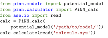
Moreover, the implementation of PiNN as an ASE calculator allows it easily to be interfaced with other codes. For example, the path integral molecular dynamics (PIMD) code i-PIKapil et al. 2019 can communicate with ASE calculators via a socket protocol, allowing PIMD simulations to be run with PiNN energies and forces.

3.4 Pressure calculations
Computing the stress tensor requires attention, especially when the potential is not pairwise-additive Thompson et al. 2009. Although an ANN potential does not look like pairwise-additive, the stress tensor calculated using the pairwise form yields the same result as the atomic form given in Ref. 55. These results were also validated using the finite difference of the potential energy with respect to the change of the volume. Therefore, the instantaneous pressure during an MD simulation is calculated as
| (10) |
where is the derivative of the potential energy with respect to the pairwise displacement vectors Martin 2013, is the momentum of atom , is the mass of that atom and is the system volume. The first term on the right hand side of the equation is the ideal gas contribution and the second term is the virial pressure output from PiNN.
3.5 Visualization of atomic neural networks with PiNNboard
It has been shown that a visualization of the activations can provide insights to their functions in convolutional neural network Zeiler and Fergus 2014. Such a visualization can also serve as a diagnostic tool to inspect and improve network architectures. Therefore, we developed a tool, PiNNboard, to visualize the activations of ANNs in atomic or pair forms. PiNNboard was implemented as a plugin for Tensorboard – TensorFlow’s visualization toolkit Abadi et al. 2016.
Here we demonstrate PiNNboard with the minimalistic PiNet, trained on a subset of the QM9 dataset containing 50604 organic molecules consisting of only C, H and O atoms. The network was trained for 3 million steps on the internal energy at 0 K () and details about the training setups can be found in the Case Studies section below.
In Fig 5, the activations of this minimalistic PiNet for the testing molecule 2,3-Dimethylfuran are visualized using PiNNboard. Colored atoms indicates the contributions of each individual atom to atomic properties. Colored bonds between atoms indicates the pairwise interactions whose contributions are significant. Indeed, most of the interactions identified by the PI layer in PiNet can be recognized as covalent bonds in Fig 5. Interestingly, strong activations in the pairwise interaction are also observed between hydrogen atoms and their second neighbors in the case of the methyl groups.

Notably, three independently trained networks (Fig 6) reach quite different atomic energy partitions as well as different pairwise interactions for the testing molecules, in spite of their identical network structure, hyper-parameters and similar mean absolute error (MAE). Therefore, one needs to be careful when interpreting atomic energies extracted from ANNs, which has also been pointed out recently Gastegger and Marquetand 2018.
We also notice that the trained network (No.1 in Fig 6) which has the smallest prediction error for the testing molecule also provides the best chemical interpretability. This suggests that not only is PiNet capable of providing a state-of-the-art performance but also the good outcome from PiNet can be rationalized in a chemically intuitive manner.
4 Case studies
For all discussed benchmarks, a network with 5 graph convolution (GC) blocks is used. The parameters are given in Table 1. Hyperbolic tangent activation functions were used in all layers, except for the output layer where a linear activation function is used for output.
Unless otherwise stated, a 80:20 dataset splitting was used for case studies, which means 80% of the structures of each dataset were randomly chosen to train the neural network, and the remaining 20% were used for validation. The Adam Kingma and Ba 2017 optimizer in TensorFlow Abadi et al. 2016 was used for gradient descent updates with a batch size of 100 samples, the training rate was set to 0.0003 and decayed by a factor of 0.994 every 100000 steps, other parameters were kept unchanged. A gradient norm clipping strategy was employed to avoid exploding gradient problems Pascanu et al. 2013. The trainings were terminated after 1-3 million gradient descent steps, which typically takes a day with a single NVIDIA TITAN V GPU card.
| Layer | Architecturea | Parameter | Value |
|---|---|---|---|
| PI | [64]10 b | 4.5 Å | |
| II | [64, 64, 64, 64] | GC blocks | 5 |
| PP | [64, 64, 64, 64] | 10 | |
| Output | [64, 1] | 3.0 |
- a
The layer architecture is denoted with the number of nodes in the hidden layers and in the output layer. [64, 64, 64, 64] means a neural network with three hidden layers, each with 64 nodes, and 64 output nodes.
- b
The PI layer does not contain any hidden layer and the output dimension of the PI layer equals to the number of elements in .
Because the purpose of PiNN is not to serve as a singular ANN architecture but to be used as a reliable and general-purpose library for further developments, we will not compare our results exhaustively with all other GCNN variants Schütt et al. 2017; Schütt et al. 2018; Xie and Grossman 2018; Lubbers et al. 2018; Unke and Meuwly 2019; Chen et al. 2019; Zubatyuk et al. 2019. Instead, SchNet Schütt et al. 2018, which pioneered the application of GCNN for modeling both molecules and materials will be quoted as the main reference to put our results into perspective.
4.1 QM9 dataset
The QM9 dataset Ramakrishnan et al. 2014 is a dataset made up of 134k small organic molecules containing computed electronic, energetic and thermodynamic properties at B3LYP/6-31G(2df,p) level of theory Becke 1993; Lee et al. 1988; Stephens et al. 1994, which is often used for benchmarking ANNs. As commonly done in the literature, 30054 structures which failed a consistency check were excluded during training and evaluationSchütt et al. 2018; Unke and Meuwly 2019.
PiNet reaches a MAE of 0.012 eV for the prediction of internal energy at 0 K, in comparison with 0.014 eV from SchNet. It is worth to mention that the so-called chemical accuracy from thermo-chemistry measurements is about 0.043 eV.
As an example of property predictions, we used PiNet to predict partial charges by regressing only the molecular dipole moment :
| (11) |
where is the predicted partial charge on atom . To ensure that the predicted total charge of each molecule is zero, we added a constraint term to the loss function.
By implementing this dipole model in PiNet, we predicted the dipole moment with an MAE of 0.018 for the QM9 dataset. The network used to predict the dipole for the QM9 dataset was trained with a learning rate of 0.0001 and batch size of 200 structures instead.
To further validate the PiNet dipole model, we also calculated partial charges using the CM5 charge model, which has been parameterized to reproduce dipole moments from experiments or high-level quantum mechanical calculations Marenich et al. 2012. The CM5 charges were calculated at the B3LYP/6-31G(2df,p) level of theory using the Gaussian packageFrisch et al., matching the original conditions in which QM9 dataset was generated. Note that CM5 charges were not used in the training of PiNet. When comparing predicted partial charges from PiNet with those from CM5 Marenich et al. 2012, a good correlation was found as shown in Fig. 7, indicating that PiNet can generate physically meaningful partial charges. This result is particularly encouraging in light of the fact that only the scalar dipole moment was used during the fitting Sifain et al. 2018.

4.2 Materials Project and Perovskite datasets
We used the dataset (“MP-crystals-2018.6.1”) provided by MEGNet Chen et al. 2019 which contains DFT-computed energies and band gaps for 69640 crystals extracted from the Materials Project Jain et al. 2013. Training of PiNet was done with 60000 crystal structures from this dataset. The trained PiNet leads to a MAE of 0.029 eV/atom for the prediction of formation energy on the test configurations, in comparison with that of 0.035 eV/atom from SchNet using the same number of structures in the training set. To put these numbers into perspective, we note that the accuracy of experimental measurement of formation energies is about 0.082 eV/atom Kirklin et al. 2015. Thus, PiNet provides also a sub-chemical accuracy for materials modeling.
In addition, PiNet was benchmarked on a dataset consisting of 18928 perovskite structures published by Castelli et al. Castelli et al. 2012. The achieved MAE of the total energy respective to the convex hull (for the purpose of assessing the thermodynamics metastability) from the trained PiNet is 0.042 eV/atom with a 60:40 splitting of the dataset. This is in comparison with the same MAE obtained from Crystal Graph Convolutional Neural Network (CGCNN) with a 80:20 splitting instead Xie and Grossman 2018. The learning curve of PiNet with this dataset is shown in Fig. 8 (in logarithm scale).

4.3 Liquid water dataset
Here we showcase the application of the BPNN implemented in PiNN to liquid water using the dataset published by Morawietz et.al Morawietz and Behler 2019 based on the BLYP functional Becke 1988; Lee et al. 1988. To facilitate the training, we also augmented this dataset using the original BPNN implementation Morawietz and Behler 2019 (See Supporting Information for details). The set of symmetry functions were chosen to match the original ones Morawietz et al. 2016, however, hyperparameters such as the learning rate and optimizer are specific in PiNN. MD simulations were performed with the Berendsen thermostat Berendsen et al. 1984 implemented in ASE and a patched Berendsen barostat (to include the missing ideal gas contribution in Eq. 10, for details see Ref. 45).
After the training, the BPNN implemented in PiNN reaches a root mean squared error (RMSE) of 7 meV/H2O for energy and 60 meV/Å for force components. These can be compared to 2 meV/H2O and 70 meV/Å for energy and force respectively, reported in Ref. 16. To validate this BPNN potential, we further carried out ab initio molecular dynamics (AIMD) simulations of the liquid water system at both NVT (constant particle, volume and temperature) and NPT (constant particle, pressure and temperature) ensembles with CP2K Hutter et al. 2013 and BLYP functional Becke 1988; Lee et al. 1988. Details of AIMD simulations can be found in the Supporting Information.

As shown in Fig 9, the BPNN potential generated with PiNN reproduces well the structure of liquid water from AIMD simulations, particularly in the NVT ensemble. It is found that at 330 K and 1 bar, this BPNN potential predicts a density of 0.74(2) g/mL, in good agreement with that of 0.79(2) g/mL from AIMD simulations. Note that the AIMD simulations shown in Fig 9 were not used in the training and merely served the purpose of the cross-validation.
4.4 Proton transfer reactions
Finally, we demonstrate that PiNet can be applied to reactive MD simulations in which covalent bonds break and form. In particular, we take the example of proton transfer reactions in aqueous NaOH solutions.
We reused and slightly modified the dataset for NaOH(aq) solutions from Ref. 74, generated with the RPBE density functionalHammer et al. 1999 and Grimme’s D3 dispersion correction Grimme et al. 2010. This dataset was originally constructed for use with BPNN and the resulting BPNN potential was tested for various thermodynamic and dynamical properties of NaOH solutions Hellström and Behler 2017; Hellström et al. 2018.

In this case, we used smaller layers in PiNet (with 16 nodes per layer rather than 64) as compared to the other case studies to prevent overfitting, and optimized the parameters primarily to minimize the error in the predicted forces. We obtained an excellent RMSE of 0.11 eV/Å for the force components for both the training and validation sets, indicating that the fit did not suffer from overfitting.
Environment-dependent proton transfer free energy profiles for NaOH solutions were calculated with PiNet (Figure 10). For each , the proton transfer coordinate is calculated as the difference in length between the hydrogen bond along which the proton is transferred, and the covalent O-H distance for the bond that becomes broken Tuckerman et al. 2002. Corresponding equilibrium MD simulations were run using an interface with the Amsterdam Modeling Suite (AMS) Rüger et al. and technical settings of MD simulations were chosen to be the same as in Ref. 74 for the sake of comparison.
Figure 10 illustrates how the free-energy landscape for proton transfer depends on the local hydrogen-bonding environments around and . Just as revealed in the previous work using BPNNs Hellström and Behler 2016 and ab initio simulations Tuckerman et al. 2002, proton transfer occurs predominately via a presolvation mechanism: mostly accepts four hydrogen bonds in its equilibrium structure, but the forward PT barrier is quite high in this case (blue curve). Instead, if via a hydrogen bond fluctuation the only accepts three hydrogen bonds (red curve), then the forward PT barrier is much smaller.
Figure 11 shows the time required to evaluate the energy and forces for different system sizes of liquid water (averaged over 100 samples), using the PiNet model parameterized for NaOH. This highlights one of the appealing features of ANNs in which the computational cost grows linearly with the number of atoms.

5 Conclusion
Here we present PiNN – an open-source Python library for building ANNs of molecules and materials. In the current version of PiNN, BPNN and our GCNN variant PiNet have been implemented and benchmarked against several publicly available datasets as well as in-house data.
Built with the TensorFlow framework, PiNN allows for fast training of ANNs with GPUs. PiNN interfaces with ASE and AMS and provides several useful package features such as analytical stress tensor calculations and a visualizer of trained ANNs called PiNNBoard.
With modularized building blocks, PiNN can be used not only as a standalone package but also as a chain of tools to develop novel ANNs. In this work, we showed how such ANNs can be used for approximating potential energy surfaces, allowing for fast and accurate reactive MD simulations, or for directly predicting several different physico-chemical properties of molecules and materials, such as dipole moments and partial charges.
In the current implementation of PiNN, the primary focus is on predicting atomic properties. In the near future, we aim to include predictions of electronic properties such as polarization as well as the coupling to the external field in periodic systems. These extensions will be quite important for modeling electrochemical systems with finite field MD simulations Zhang et al. 2019; Zhang et al. 2016. Moreover, we are interested in incorporating active learning and on-the-fly potential generation.
Last but not least, PiNN will take advantage of the evolving TensorFlow ecosystem which allows to access novel optimization methods implemented in its peripheral packages such as K-FAC (Kronecker-Factored Approximated Curvature) Martens and Grosse 2015 for fast training of ANNs.
Details of liquid water dataset augmentation and AIMD simulations of liquid water.
References
- Dirac (1929) Dirac, P. A. M. Quantum mechanics of many-electron systems. Proc. R. Soc. London, Ser. A 1929, 123, 714–733.
- Bartók et al. (2017) Bartók, A. P.; De, S.; Poelking, C.; Bernstein, N.; Kermode, J. s. R.; Csányi, G.; Ceriotti, M. Machine learning unifies the modeling of materials and molecules. Sci. Adv. 2017, 3, e1701816.
- Aspuru-Guzik et al. (2018) Aspuru-Guzik, A.; Lindh, R.; Reiher, M. The Matter Simulation (R)evolution. ACS Cent. Sci. 2018, 4, 144–152.
- Butler et al. (2018) Butler, K. T.; Davies, D. W.; Cartwright, H.; Isayev, O.; Walsh, A. Machine learning for molecular and materials science. Nature 2018, 559, 1–9.
- Behler and Parrinello (2007) Behler, J.; Parrinello, M. Generalized Neural-Network Representation of High-Dimensional Potential-Energy Surfaces. Phys. Rev. Lett. 2007, 98, 146401.
- Schütt et al. (2017) Schütt, K. T.; Arbabzadah, F.; Chmiela, S.; Müller, K.-R.; Tkatchenko, A. Quantum-chemical insights from deep tensor neural networks. Nat. Commun. 2017, 8, 13890.
- Gassner et al. (1998) Gassner, H.; Probst, M.; Lauenstein, A.; Hermansson, K. Representation of Intermolecular Potential Functions by Neural Networks. J. Phys. Chem. A 1998, 102, 4596–4605.
- Behler (2011) Behler, J. Atom-centered symmetry functions for constructing high-dimensional neural network potentials. J. Chem. Phys. 2011, 134, 074106.
- Behler (2015) Behler, J. Constructing High-Dimensional Neural Network Potentials: A Tutorial Review. Int. J. Quantum Chem. 2015, 115, 1032–1050.
- Smith et al. (2017) Smith, J. S.; Isayev, O.; Roitberg, A. E. ANI-1: an extensible neural network potential with DFT accuracy at force field computational cost. Chem. Sci. 2017, 8, 3192–3203.
- Gastegger et al. (2017) Gastegger, M.; Behler, J.; Marquetand, P. Machine learning molecular dynamics for the simulation of infrared spectra. Chem. Sci. 2017, 8, 6924–6935.
- Yao et al. (2018) Yao, K.; Herr, J. E.; Toth, D. W.; Mckintyre, R.; Parkhill, J. The TensorMol-0.1 model chemistry: a neural network augmented with long-range physics. Chem. Sci. 2018, 9, 2261–2269.
- Schran et al. (2018) Schran, C.; Uhl, F.; Behler, J.; Marx, D. High-dimensional neural network potentials for solvation: The case of protonated water clusters in helium. J. Chem. Phys. 2018, 148, 102310.
- Khaliullin et al. (2011) Khaliullin, R. Z.; Eshet, H.; Kühne, T. D.; Behler, J.; Parrinello, M. Nucleation mechanism for the direct graphite-to-diamond phase transition. Nat. Mater. 2011, 10, 693–697.
- Artrith and Kolpak (2015) Artrith, N.; Kolpak, A. M. Grand canonical molecular dynamics simulations of Cu-Au nanoalloys in thermal equilibrium using reactive ANN potentials. Comput. Mater. Sci. 2015, 110, 20.
- Morawietz et al. (2016) Morawietz, T.; Singraber, A.; Dellago, C.; Behler, J. How van der Waals interactions determine the unique properties of water. Proc. Natl. Acad. Sci. U.S.A 2016, 113, 8368–8373.
- Hellström et al. (2019) Hellström, M.; Quaranta, V.; Behler, J. One-dimensional vs. two-dimensional proton transport processes at solid–liquid zinc-oxide–water interfaces. Chem. Sci. 2019, 10, 1232–1243.
- Krizhevsky et al. (2012) Krizhevsky, A.; Sutskever, I.; Hinton, G. E. ImageNet classification with deep convolutional neural networks. Advances in Neural Information Processing Systems. 2012; pp 1097–1105.
- Duvenaud et al. (2015) Duvenaud, D.; Maclaurin, D.; Aguilera-Iparraguirre, J.; Gómez-Bombarelli, R.; Hirzel, T. i.; Aspuru-Guzik, A.; Adams, R. P. Convolutional networks on graphs for learning molecular fingerprints. Advances in Neural Information Processing Systems. 2015; pp 2224–2232.
- Kearnes et al. (2016) Kearnes, S.; McCloskey, K.; Berndl, M.; Pande, V.; Riley, P. Molecular graph convolutions: moving beyond fingerprints. J. Comput. Aided Mol. Des. 2016, 30, 595–608.
- Schütt et al. (2018) Schütt, K. T.; Sauceda, H. E.; Kindermans, P.-J.; Tkatchenko, A.; Müller, K.-R. SchNet — A deep learning architecture for molecules and materials. J. Chem. Phys. 2018, 148, 241722.
- Xie and Grossman (2018) Xie, T.; Grossman, J. C. Crystal Graph Convolutional Neural Networks for an Accurate and Interpretable Prediction of Material Properties. Phys. Rev. Lett. 2018, 120, 145301.
- Lubbers et al. (2018) Lubbers, N.; Smith, J. S.; Barros, K. Hierarchical modeling of molecular energies using a deep neural network. J. Chem. Phys. 2018, 148, 241715.
- Unke and Meuwly (2019) Unke, O. T.; Meuwly, M. PhysNet: A Neural Network for Predicting Energies, Forces, Dipole Moments, and Partial Charges. J. Chem. Theory Comput. 2019, 15, 3678–3693.
- Chen et al. (2019) Chen, C.; Ye, W.; Zuo, Y.; Zheng, C.; Ong, S. P. Graph Networks as a Universal Machine Learning Framework for Molecules and Crystals. Chem. Mater. 2019, 31, 3564–3572.
- Zubatyuk et al. (2019) Zubatyuk, R.; Smith, J. S.; Leszczynski, J.; Isayev, O. Accurate and transferable multitask prediction of chemical properties with an atoms-in-molecules neural network. Sci. Adv. 2019, 5, eaav6490.
- Chen et al. (2018) Chen, X.; Jørgensen, M. S.; Li, J.; Hammer, B. Atomic Energies from a Convolutional Neural Network. J. Chem. Theory Comput. 2018, 14, 3933–3942.
- Schütt et al. (2019) Schütt, K. T.; Gastegger, M.; Tkatchenko, A.; Müller, K.-R. In Explainable AI: Interpreting, Explaining and Visualizing Deep Learning; Samek, W., Montavon, G., Vedaldi, A., Hansen, L. K., Müller, K.-R., Eds.; Springer International Publishing: Cham, 2019; pp 311–330.
- Khorshidi and Peterson (2016) Khorshidi, A.; Peterson, A. A. Amp: A modular approach to machine learning in atomistic simulations. Comput. Phys. Commun. 2016, 207, 310–324.
- Artrith and Urban (2016) Artrith, N.; Urban, A. An implementation of artificial neural-network potentials for atomistic materials simulations: Performance for TiO2. Comput. Mater. Sci. 2016, 114, 135–150.
- Wang et al. (2018) Wang, H.; Zhang, L.; Han, J.; E, W. DeePMD-kit: A deep learning package for many-body potential energy representation and molecular dynamics. Comput. Phys. Commun. 2018, 228, 178–184.
- Singraber et al. (2019) Singraber, A.; Behler, J.; Dellago, C. Library-Based LAMMPS Implementation of High-Dimensional Neural Network Potentials. J. Chem. Theory Comput. 2019, 15, 1827–1840.
- Schütt et al. (2019) Schütt, K. T.; Kessel, P.; Gastegger, M.; Nicoli, K. A.; Tkatchenko, A.; Müller, K.-R. SchNetPack: A Deep Learning Toolbox For Atomistic Systems. J. Chem. Theory Comput. 2019, 15, 448–455.
- Huang and Von Lilienfeld (2016) Huang, B.; Von Lilienfeld, O. A. Communication: Understanding molecular representations in machine learning: The role of uniqueness and target similarity. J. Chem. Phys. 2016, 145, 161102.
- Gastegger et al. (2018) Gastegger, M.; Schwiedrzik, L.; Bittermann, M.; Berzsenyi, F.; Marquetand, P. wACSF—Weighted atom-centered symmetry functions as descriptors in machine learning potentials. J. Chem. Phys. 2018, 148, 241709.
- Faber et al. (2018) Faber, F. A.; Christensen, A. S.; Huang, B.; Von Lilienfeld, O. A. Alchemical and structural distribution based representation for universal quantum machine learning. J. Chem. Phys. 2018, 148, 241717.
- Zhang et al. (2018) Zhang, L.; Han, J.; Wang, H.; Car, R.; E, W. Deep Potential Molecular Dynamics: A Scalable Model with the Accuracy of Quantum Mechanics. Phys. Rev. Lett. 2018, 120, 143001.
- Willatt et al. (2019) Willatt, M. J.; Musil, F.; Ceriotti, M. Atom-density representations for machine learning. J. Chem. Phys. 2019, 150, 154110.
- Bartók et al. (2013) Bartók, A. P.; Kondor, R.; Csányi, G. On representing chemical environments. Phys. Rev. B 2013, 87, 184115.
- Drautz (2019) Drautz, R. Atomic cluster expansion for accurate and transferable interatomic po tentials. Phys. Rev. B 2019, 99, 014104.
- Glielmo et al. (2018) Glielmo, A.; Zeni, C.; De Vita, A. Efficient nonparametric -body force fields from machine learning. Phys. Rev. B 2018, 97, 184307.
- Gilmer et al. (2017) Gilmer, J.; Schoenholz, S. S.; Riley, P. F.; Vinyals, O.; Dahl, G. E. Neural Message Passing for Quantum Chemistry. Proceedings of the 34th International Conference on Machine Learning - Volume 70. 2017; pp 1263–1272.
- Xu et al. (2019) Xu, K.; Hu, W.; Leskovec, J.; Jegelka, S. How Powerful are Graph Neural Networks? International Conference on Learning Representations. 2019.
- Abadi et al. (2016) Abadi, M. et al. TensorFlow: Large-Scale Machine Learning on Heterogeneous Distributed Systems. 2016.
- (45) PiNN documentation. https://teoroo-pinn.readthedocs.io/en/latest, Accessed: 2019-10-08.
- Ramakrishnan et al. (2014) Ramakrishnan, R.; Dral, P. O.; Rupp, M.; Von Lilienfeld, O. A. Quantum chemistry structures and properties of 134 kilo molecules. Sci. Data 2014, 1, 140022.
- Smith et al. (2017) Smith, J. S.; Isayev, O.; Roitberg, A. E. ANI-1, A data set of 20 million calculated off-equilibrium conformations for organic molecules. Sci. Data 2017, 4, 170193.
- van der Walt et al. (2011) van der Walt, S.; Colbert, S. C.; Varoquaux, G. The NumPy Array: A Structure for Efficient Numerical Computation. Comput. Sci. Eng. 2011, 13, 22–30.
- Larsen et al. (2017) Larsen, A. H. et al. The atomic simulation environment—a Python library for working with atoms. J. Phys. Condens. Matter 2017, 29, 273002.
- Behler (2017) Behler, J. First Principles Neural Network Potentials for Reactive Simulations of Large Molecular and Condensed Systems. Angew. Chem. Int. Edit. 2017, 56, 12828–12840.
- Hutter et al. (2013) Hutter, J.; Iannuzzi, M.; Schiffmann, F.; VandeVondele, J. CP2K: atomistic simulations of condensed matter systems. Wiley Interdiscip. Rev. Comput. Mol. Sci. 2013, 4, 15–25.
- (52) Rüger, R.; Franchini, M.; Trnka, T.; Yakovlev, A.; van Lenthe, E.; Philipsen, P.; Klumpers, B.; Soini, T. AMS 2019. http://www.scm.com, SCM, Theoretical Chemistry, Vrije Universiteit, Amsterdam, The Netherlands.
- Allen and Tildesley (2017) Allen, M. P.; Tildesley, D. J. Computer Simulation of Liquids: Second Edition; Oxford University Press, 2017.
- Kapil et al. (2019) Kapil, V. et al. i-PI 2.0: A universal force engine for advanced molecular simulations. Comput. Phys. Commun. 2019, 236, 214–223.
- Thompson et al. (2009) Thompson, A. P.; Plimpton, S. J.; Mattson, W. General formulation of pressure and stress tensor for arbitrary many-body interaction potentials under periodic boundary conditions. J. Chem. Phys. 2009, 131, 154107.
- Martin (2013) Martin, R. M. Electronic Structure: Basic Theory and Practical Methods; Cambridge University Press: Cambridge, 2013.
- Zeiler and Fergus (2014) Zeiler, M. D.; Fergus, R. Visualizing and Understanding Convolutional Networks. Computer Vision – ECCV 2014. Cham, 2014; pp 818–833.
- Gastegger and Marquetand (2018) Gastegger, M.; Marquetand, P. Molecular Dynamics with Neural-Network Potentials. arXiv:1812.07676 [physics, stat] 2018, arXiv: 1812.07676.
- Kingma and Ba (2017) Kingma, D. P.; Ba, J. Adam: A Method for Stochastic Optimization. arXiv:1412.6980 [cs] 2017, arXiv: 1412.6980.
- Pascanu et al. (2013) Pascanu, R.; Mikolov, T.; Bengio, Y. On the Difficulty of Training Recurrent Neural Networks. Proceedings of the 30th International Conference on International Conference on Machine Learning - Volume 28. 2013; pp 1310–1318.
- Becke (1993) Becke, A. D. Density-functional thermochemistry. III. The role of exact exchange. J. Chem. Phys. 1993, 98, 5648–5652.
- Lee et al. (1988) Lee, C.; Yang, W.; Parr, R. G. Development of the Colle-Salvetti correlation-energy formula into a functional of the electron density. Phys. Rev. B 1988, 37, 785–789.
- Stephens et al. (1994) Stephens, P. J.; Devlin, F. J.; Chabalowski, C. F.; Frisch, M. J. Ab Initio Calculation of Vibrational Absorption and Circular Dichroism Spectra Using Density Functional Force Fields. J. Phys. Chem. 1994, 98, 11623–11627.
- Marenich et al. (2012) Marenich, A. V.; Jerome, S. V.; Cramer, C. J.; Truhlar, D. G. Charge Model 5: An Extension of Hirshfeld Population Analysis for the Accurate Description of Molecular Interactions in Gaseous and Condensed Phases. J. Chem. Theory Comput. 2012, 8, 527–541.
- (65) Frisch, M. J. et al. Gaussian 09 Revision D.01. Gaussian Inc. Wallingford CT 2009.
- Sifain et al. (2018) Sifain, A. E.; Lubbers, N.; Nebgen, B. T.; Smith, J. S.; Lokhov, A. Y.; Isayev, O. e.; Roitberg, A. E.; Barros, K.; Tretiak, S. Discovering a Transferable Charge Assignment Model Using Machine Learning. J. Phys. Chem. Lett. 2018, 9, 4495–4501.
- Jain et al. (2013) Jain, A.; Ong, S. P.; Hautier, G.; Chen, W.; Richards, W. D.; Dacek, S.; Cholia, S.; Gunter, D.; Skinner, D.; Ceder, G.; Persson, K. a. The Materials Project: A materials genome approach to accelerating materials innovation. APL Mater. 2013, 1, 011002.
- Kirklin et al. (2015) Kirklin, S.; Saal, J. E.; Meredig, B.; Thompson, A.; Doak, J. W.; Aykol, M.; Rühl, S.; Wolverton, C. The Open Quantum Materials Database (OQMD): assessing the accuracy of DFT formation energies. Npj Comput. Mater. 2015, 1, 15010.
- Castelli et al. (2012) Castelli, I. E.; Olsen, T.; Datta, S.; Landis, D. D.; Dahl, S.; Thygesen, K. S.; Jacobsen, K. W. Computational screening of perovskite metal oxides for optimal solar light capture. Energy Environ. Sci. 2012, 5, 5814–5819.
- Xie and Grossman (2018) Xie, T.; Grossman, J. C. Hierarchical visualization of materials space with graph convolutional neural networks. J. Chem. Phys. 2018, 149, 174111.
- Morawietz and Behler (2019) Morawietz, T.; Behler, J. HDNNP training data set for H2O. 2019; https://zenodo.org/record/2634098.
- Becke (1988) Becke, A. D. Density-functional exchange-energy approximation with correct asymptotic behavior. Phys. Rev. A 1988, 38, 3098–3100.
- Berendsen et al. (1984) Berendsen, H. J. C.; Postma, J. P. M.; van Gunsteren, W. F.; DiNola, A.; Haak, J. R. Molecular dynamics with coupling to an external bath. J. Chem. Phys. 1984, 81, 3684–3690.
- Hellström and Behler (2016) Hellström, M.; Behler, J. Concentration-Dependent Proton Transfer Mechanisms in Aqueous NaOH Solutions: From Acceptor-Driven to Donor-Driven and Back. J. Phys. Chem. Lett. 2016, 7, 3302–3306.
- Hammer et al. (1999) Hammer, B.; Hansen, L. B.; Nørskov, J. K. Improved adsorption energetics within density-functional theory using revised Perdew-Burke-Ernzerhof functionals. Phys. Rev. B 1999, 59, 7413–7421.
- Grimme et al. (2010) Grimme, S.; Antony, J.; Ehrlich, S.; Krieg, H. A consistent and accurate ab initio parametrization of density functional dispersion correction (DFT-D) for the 94 elements H-Pu. J. Chem. Phys. 2010, 132, 154104.
- Hellström and Behler (2017) Hellström, M.; Behler, J. Structure of aqueous NaOH solutions: insights from neural-network-based molecular dynamics simulations. Phys. Chem. Chem. Phys. 2017, 19, 82–96.
- Hellström et al. (2018) Hellström, M.; Ceriotti, M.; Behler, J. Nuclear Quantum Effects in Sodium Hydroxide Solutions from Neural Network Molecular Dynamics Simulations. J. Phys. Chem. B 2018, 122, 10158–10171.
- Tuckerman et al. (2002) Tuckerman, M. E.; Marx, D.; Parrinello, M. The nature and transport mechanism of hydrated hydroxide ions in aqueous solution. Nature 2002, 417, 925–929.
- Zhang et al. (2019) Zhang, C.; Hutter, J.; Sprik, M. Coupling of Surface Chemistry and Electric Double Layer at TiO2 Electrochemical Interfaces. J. Phys. Chem. Lett. 2019, 10, 3871–3876.
- Zhang et al. (2016) Zhang, C.; Hutter, J.; Sprik, M. Computing the Kirkwood g-Factor by Combining Constant Maxwell Electric Field and Electric Displacement Simulations: Application to the Dielectric Constant of Liquid Water. J. Phys. Chem. Lett. 2016, 7, 2696–2701.
- Martens and Grosse (2015) Martens, J.; Grosse, R. Optimizing Neural Networks with Kronecker-Factored Approximate Curvature. Proceedings of the 32nd International Conference on International Conference on Machine Learning - Volume 37. 2015; pp 2408–2417.