Topology-Induced Spontaneous Non-reciprocal Pumping in Cold-Atom Systems with Loss

Linhu Li Email: phylli@nus.edu.sg Affiliation: Department of Physics, National University of Singapore, Singapore 117551, Republic of Singapore Ching Hua Lee Email: calvin-lee@ihpc.a-star.edu.sg Affiliation: Institute of High Performance Computing, A*STAR, Singapore, 138632. Affiliation: Department of Physics, National University of Singapore, Singapore 117551, Republic of Singapore Jiangbin Gong Email: phygj@nus.edu.sg Affiliation: Department of Physics, National University of Singapore, Singapore 117551, Republic of Singapore

August 11, 2026

Abstract

We propose a realistic cold-atom quantum setting where nontrivial energy-band topology induces non-reciprocal pumping. This is an intriguing non-Hermitian phenomenon that illustrates how topology, when assisted with atom loss, can act as a “switch” for non-Hermitian skin effect (NHSE), rather than as a passive property that is modified by the NHSE. In particular, we present a lattice-shaking scenario to realize a two-dimensional cold-atom platform, where non-reciprocity is switched on only in the presence of both atom loss and topological localization due to time-reversal symmetry breaking. Such spontaneous non-reciprocal pumping is manifested by asymmetric dynamical evolution, detectable by atomic populations along the system edges. Our results may trigger possible applications in non-reciprocal atomtronics, where loss and topological mechanisms conspire to control atomic transport.

Introduction. – Cold atoms on optical lattices provide a highly promising platform for demonstrating interesting topological and many-body physics Bloch et al. 2008; Goldman et al. 2016. Recent advances in lattice shaking technology have enabled unprecedented tuning of effective tunneling amplitudes, leading to pioneering observations of various exotic topological states Lignier et al. 2007; Struck et al. 2011; Struck et al. 2012; Hauke et al. 2012; Jotzu et al. 2014; Kang et al. 2018; Kang et al.. Beyond realizing conventional static and Floquet topological phases Goldman et al. 2010; Liu et al. 2013a; Liu et al. 2013b; Liu et al. 2014; Potirniche et al. 2017; Li et al. 2018a; Lee et al. 2018; Zhou and Gong 2018; Yang et al. 2018, cold-atoms in optical systems are also suitable quantum platforms for simulating higher-order topological phases Benalcazar et al. 2017a; Benalcazar et al. 2017b; Schindler et al. 2018; Wang et al. 2018; Zeng et al. 2019; Luo and Zhang 2019 and non-Hermitian effects Bender and Boettcher 1998; Rotter 2009a; Li et al. 2019a, two classes of phenomena of intense current interest. Indeed, non-Hermiticity can be experimentally implemented through optically-induced depopulating losses Li et al. 2019a, and be fine-tuned to exhibit non-Hermitian topological degeneracies Xu et al. 2017; Luo and Zhang 2019 like exceptional points Berry 2004; Rotter 2009b; Heiss 2012; Hassan et al. 2017; Hu et al. 2017, lines Xu et al. 2017; Carlström and Bergholtz 2018; Moors et al. 2019; Wang et al. 2019; Yang and Hu 2019; Carlström et al. 2019; Yoshida et al. 2019; Luo et al.; Yoshida and Hatsugai and surfaces Zhou et al. 2019; Okugawa and Yokoyama 2019, all possessing rich geometric structure without Hermitian analogs Shen et al. 2018; Yin et al. 2018; Li et al. 2019b.

In this work, we propose the cold-atom realization of a novel phenomenon where topological localization in one direction spontaneously breaks the reciprocity of a two-dimensional (2D) lattice system in the presence of atom loss, leading to non-reciprocal pumping in the transverse direction. This is orthogonal in spirit to much contemporary theoretical Yao and Wang 2018; Kunst et al. 2018; Xiong 2018; Jin and Song 2019; Lee and Thomale 2019; Lee et al.; Song et al. 2019a; Longhi 2019a; Longhi 2019b and experimental Helbig et al.; Hofmann et al.; Ghatak et al.; Xiao et al. literature, which focuses on the breakdown of conventional topological bulk-boundary correspondences (BBCs) caused by non-reciprocal pumping i.e. the non-Hermitian skin effect (NHSE). Our proposal instead illustrates how nontrivial topology can conversely cause non-reciprocal pumping, as illustrated in Fig. 1(e). The resultant topology-induced NHSE pumping, with non-Hermiticity implemented via atom loss only, is marked by corner mode accumulation scaling extensively with the system length Lee et al. 2019, fundamentally unlike higher-order topological corner modes, Hermitian or otherwise Liu et al. 2019; Edvardsson et al. 2019; Ezawa; Liu et al. 2018; Luo and Zhang 2019. Our results may stimulate further work on non-reciprocal atomtronics, exploiting both atom loss and topological mechanisms to control atomic transport. Relying on a quantum platform, our proposal is also intrinsically poised for further exploring non-Hermitian effects with tunable many-body interactions.

Our setup consists of an optically shaken lattice accommodating cold atoms, designed such that lattice anisotropy and antiphase shaking conspire to yield nontrivial first-order topology generating one-dimensional (1D) topological edge modes. The required atom loss is introduced through selective depopulation, by exciting the atoms into an excited state with a resonant beam. Due to the extreme robustness of both Chern topology and the resultant nonreciprocal pumping, our topology-induced corner modes are stable across a large region in the parameter space, as evident in Fig. 3(e). They can be distinguished from higher-order topological corner modes via their asymmetric dynamical evolution arising from tspontaneously broken reciprocity (Fig. 4).

2D optical lattice and model Hamiltonian. – Consider a gas of Fermionic atoms in a two-frequency periodically driven 2D superlattice formed by three directed optical standing waves, described by the potential [Fig. 1(a)]

	$\displaystyle V(x,y)=2V_{y}\left[\sin^{2}\left(\frac{2\pi}{\lambda_{L}}y\right)+\cos^{2}\left(\frac{4\pi}{\lambda_{L}}y\right)\right]$	(1)
$\displaystyle+$	$\displaystyle 2V_{-}(\omega_{2}t)\cos^{2}\{\frac{2\pi}{\lambda_{L}}[\beta(x-x_{1}(\omega_{1}t))+y/2]+\frac{\pi}{4}\}$
$\displaystyle+$	$\displaystyle 2V_{+}(\omega_{2}t)\sin^{2}\{\frac{2\pi}{\lambda_{L}}[\beta(x-x_{1}(\omega_{1}t))-y/2]+\frac{\pi}{4}\},$

where $\lambda_{L}/2$ sets the lattice constant along the $y$ -direction. $V_{y}$ describes a static double-well potential along the $y$ -direction, realizable with two pairs of interfering laser beams Peil et al. 2003; Fölling et al. 2007; Trotzky et al. 2008; Atala et al. 2013. The other two potentials with coefficients $V_{\pm}$ have oblique orientations determined by $\beta$ , and are time-dependent with oscillations controlled by frequency $\omega_{1}$ through $x_{1}(\omega_{1}t)=-d_{1}\cos\omega_{1}t$ , induced by sinusoidally modulating the frequency difference between the interfering laser beams Gemelke et al. 2005; Lignier et al. 2007; Zheng and Zhai 2014; Zhang and Zhou 2014; Kang et al.; and small-amplitude driving with frequency $\omega_{2}$ through $V_{\pm}(\omega_{2}t)=V_{xy}[1\pm A\cos(\omega_{2}t+\varphi)]/2$ , $|A|\leqslant 1$ . These dynamical potential modulations of dissimilar frequencies break TR symmetry, and can induce Chern topology. In particular, the oppositely modulated $V_{\pm}$ amplitudes gives rise to a lattice of potential minima $x_{0}^{\tau}(t)$ with its two sublattices $\tau=a,b$ (white, gray) shaken in opposite directions [arrows in Fig. 1(b)]: $x^{\tau}_{0}(t)=x_{1}(t)-d_{2}\cos(\omega_{2}t+\varphi_{\tau})$ , where $\varphi_{a}=\varphi_{b}+\pi=\varphi$ and effective shaking amplitude $d_{2}\approx\frac{d}{2\beta\pi}\tan^{-1}\left[\sqrt{5/3}A\right]$ Sup. While our setup is valid for generic parameter values, we shall set $\beta=1$ , $\lambda_{L}=532$ nm in the numerics that follow, and consider small shaking amplitudes $d_{2}=d_{1}/20=\lambda_{L}/200$ ¹¹ 1 Larger amplitudes lead to a greater number of nontrivial couplings without necessarily introducing new physics..

Refer to caption — Figure 1: (a) 2D optical lattice depicted by Eq. 1, with snapshot taken when $x_{1}(\omega_{1}t)=0$ and $V_{-}(\omega_{2}t)=V_{+}(\omega_{2}t)=V_{y}/2$ . (b) The corresponding lattice structure of (a), with its two sublattices shaken in opposite directions (black arrows). (c) Effective 1D potential experienced by each sublattice along the $x$ direction, with $|\uparrow\rangle$ and $|\downarrow\rangle$ pseudospins representing the $s$ and $p_{x}$ orbitals. Atoms in the $|\downarrow\rangle$ state are resonantly excited to a third state $|e\rangle$ , leading to loss. (d) Two-leg system (Eq. 3) for each sublattice (white/gray rows in Fig. 1(b)), with yellow/green sites representing up/down pseudospins. (e) Mechanism for topology-induced non-reciprocal corner modes. The reciprocity of the lattice is spontaneously broken when topological boundary modes localize on the upper/lower sublattices along the upper/lower edge, such that non-reciprocal pumping towards the right/left dominates.

To obtain a suitable effective tight-binding Hamiltonian, we consider (unless otherwise stated) bi-chromatic driving Kang et al. with resonant frequency values $\omega_{2}=2\omega_{1}\approx\epsilon_{sp_{x}}/\hbar$ , $\epsilon_{sp_{x}}$ the on-site energy difference between the $s$ and $p_{x}$ orbitals of the fermions. These orbitals are in turn coupled by two-photon inter-orbital resonant couplings Zheng and Zhai 2014; Zhang and Zhou 2014; Kang et al. arising from a momentum term induced by $x$ -direction shaking, which do not couple different $p_{y}$ orbitals. As such, $p_{y}$ orbitals are decoupled from the $p_{x}$ and $s$ orbitals, labeled as pseudospins $|\uparrow\rangle$ and $|\downarrow\rangle$ respectively. Finally, to introduce nontrivial non-Hermiticity, on-site atom loss is asymmetrically introduced on the $|\downarrow\rangle$ state by using a resonant optical beam to transfer the atoms to an excited state $|e\rangle$ [Fig. 1(c)] Li et al. 2019a.

In the high frequency regime with small oscillation amplitudes, the Magnus expansion approximation gives the effective static Hamiltonian $H({\bm{k}})=\Psi^{\dagger}({\bm{k}})h_{\rm 2D}({\bm{k}})\Psi({\bm{k}})$ with $\Psi^{\dagger}({\bm{k}})=(\hat{a}^{\dagger}_{\uparrow{\bm{k}}},\hat{b}^{\dagger}_{\uparrow{\bm{k}}},\hat{a}^{\dagger}_{\downarrow{\bm{k}}},\hat{b}^{\dagger}_{\downarrow{\bm{k}}})$ creating states on $a,b$ sublattices and $|\uparrow\rangle,|\downarrow\rangle$ pseudospins, and Sup

\displaystyle h_{\rm 2D}(\bm{k})

\displaystyle=

\displaystyle h^{+}_{\sigma}(\bm{k})\sigma_{0}+h^{-}_{\sigma}(\bm{k})\sigma_{3}+h^{+}_{\tau}(\bm{k})\tau_{0}+h^{-}_{\tau}(\bm{k})\tau_{3},

	$\displaystyle h^{\pm}_{\sigma}(\bm{k})$	$\displaystyle=$	$\displaystyle-(2t_{\pm,x}\cos k_{x}-\Delta_{\pm}\pm ig)\tau_{0}-\{t_{\pm,y}+t^{\prime}_{\pm,y}[\cos k_{y}+\cos(k_{y}-k_{x})]\}\tau_{1}-t^{\prime}_{\pm,y}[\sin k_{y}+\sin(k_{y}-k_{x})]\tau_{2},$
	$\displaystyle h^{-}_{\tau}(\bm{k})$	$\displaystyle=$	$\displaystyle(t_{v}\cos\varphi)\sigma_{1}+(t_{v}\sin\varphi)\sigma_{2},~h^{+}_{\tau}(\bm{k})=(2t_{d}\sin k_{x})\sigma_{2},$		(3)

$\tau_{i}$ and $\sigma_{i}$ ( $i=1,2,3$ ) two sets of Pauli matrices acting on the sublattice and pseudospin spaces respectively, with $\tau_{0}$ and $\sigma_{0}$ their corresponding two by two identity matrices. The various coupling amplitudes $t_{v},t_{d}$ , $t_{\pm,\alpha}=(t_{\uparrow,\alpha}\pm t_{\downarrow,\alpha})/2$ and $t^{\prime}_{\pm,\alpha}=(t^{\prime}_{\uparrow,\alpha}\pm t^{\prime}_{\downarrow,\alpha})/2$ arise from overlap integrals between the atomic orbitals, as detailed in the Supplementary Material Sup. Since these couplings do not connect different pseudospin and sublattice components simultaneously, $h_{\rm 2D}(\bm{k})$ can be visualized as the lattice in Fig. 1(b) with each $\tau\in\{a,b\}$ row represented by a two-leg lattice with couplings between $s$ and $p_{x}$ orbitals differing by a $\pi$ phase i.e. $\varphi_{a}=\varphi_{b}+\pi$ ( Fig. 1(d)). The shaking-induced inter-orbital coupling $t_{v}$ and $t_{d}$ breaks the TR and inversion symmetries respectively, giving rise to Chern topology Jotzu et al. 2014. Note that, non-Hermiticity enters here through $-ig\tau_{0}(\sigma_{0}-\sigma_{3})$ , depicting a loss mechanism acting only on the $|\downarrow\rangle$ pseudospin sector. This pseuedospin down sector is energetically offset from the $|\uparrow\rangle$ sector by $\Delta_{-}$ . There is no atom gain introduced to the system. The $\Delta_{+}$ term represents an overall energy shift that we can be neglected). For concreteness in our numerics, we have considered a lattice loaded with a Fermionic gas of ¹⁷³Yb atoms, although our scheme is also applicable for other cold atoms.

Edge modes from topological localization. – In the static ( $\omega_{1}=\omega_{2}=0$ ) Hermitian limit, our $h_{\rm 2D}(\bm{k})$ system posseses sublattice symmetry, and is topologically nontrivial with $Z$ -quantized 1D Berry phase

\displaystyle\gamma^{y}_{n}(k_{x})=-{\rm Im}\oint_{0}^{2\pi}dk_{y}\langle u_{n}(k_{x},k_{y})|\partial_{k_{y}}|u_{n}(k_{x},k_{y})\rangle

(4)

for each $n$ -th band $|u_{n}(k_{x},k_{y})\rangle$ . When TR symmetry is broken through lattice shaking at nonzero $\omega_{2}=2\omega_{1}$ Sup, its resultant topological boundary modes along the $y$ -edge crossover to Chern chiral edge modes, analogous to the zigzag-edge edge modes of Graphene or other honeycomb lattices under a circularly polarized laser Usaj et al. 2014; Perez-Piskunow et al. 2014; Sentef et al. 2015. As evident in Fig. 2 with open boundary conditions (OBCs) along $y$ , these Chern edge states (red) are however only weakly separated due to the small shaking amplitudes and hence small inter-pseudospin coupling. This weak coupling also yields almost quantized Berry phases $\gamma_{1}^{y}$ and $\gamma_{4}^{y}$ shown in Fig. 2. The average Berry phase $\bar{\gamma}^{y}_{n}=\sum_{k_{x}}\gamma^{y}_{n}(k_{x})/N_{x}$ used later gives the ratio of the total number of 1D edge modes to $N_{x}$ under $x$ -PBC/ $y$ -OBC, which turns out to be proportional to the corner mode accumulation strength Lee et al. 2019 and hence spontaneous non-reciprocal pumping elaborated below.

Topology-induced nonreciprocal corner modes.– The non-Hermiticity introduced by on-site atom loss does not merely perturb the spectrum to complex values [Fig. 3(a)]. Interestingly, it also produces strong mode accumulation at two opposite corners, as conceptually sketched in Fig. 1(e) and quantitatively plotted in Fig. 3(b). Fundamentally unlike corner modes arising from higher-order topology, our corner mode density scales extensively with the system length, as elucidated in Fig. 3(c) by the linear scaling behavior of the total mode intensity $\rho_{\text{sum}}(x,y)=\sum_{n,\sigma}|\psi_{n}(\sigma,x,y)|^{2}$ with system length $N_{x}$ at the nontrivial corner $(x,y)=(N_{x},1)$ . (or at the other corner $(1,N_{y})$ , not shown). Since the number of topological boundary modes is fixed by the topological invariant, this extensive scaling of mode intensity must have alternatively originated from some form of the NHSE ²² 2 The NHSE is characterized by extensive mode accumulation along a boundary in the simultaneous presence of non-reciprocity and non-Hermiticity.. Indeed, we have realized one form of hybrid corner modes Lee et al. 2019 by exploiting atom loss.

To understand this enigmatic corner mode accumulation, first note that the loss term $-ig\tau_{0}(\sigma_{0}-\sigma_{3})$ in the $|\downarrow\rangle$ sector hardly changes the topological modes, as evident from comparing the Re $[E]$ inset of Fig. 3(a) with the dissipationless bandstructure in Fig. 2. With chosen experimental parameters producing considerably weak inter-orbital couplings $t_{v}$ and $t_{d}$ , one can also largely confine the damping effects within the $|\downarrow\rangle$ sector (orange in Fig. 3(a) with large -Im $[E]$ ), and observe non-reciprocal effects in the $|\uparrow\rangle$ sector possessing almost real eigenenergies.

We can obtain intuition about how these non-reciprocal effects can be topology-induced from a Gedanken experiment of tuning the couplings $(t_{\sigma,y},t^{\prime}_{\sigma,y})\rightarrow c(t_{\sigma,y},t^{\prime}_{\sigma,y})$ , where $c\in[0,1]$ interpolates between the decoupled limit and the full values of these couplings. In the fictitious $c=0$ decoupled limit, $t_{\sigma,y}=t^{\prime}_{\sigma,y}=0$ , and the system is decoupled into a series of 1D two-leg ladders as in Fig. 1(d), with $\varphi_{a,b}$ differing by $\pi$ between the sublattices $a$ and $b$ . Upon rotating $\sigma_{1}$ , $\sigma_{2}$ and $\sigma_{3}$ , the decoupled 1D two-leg ladders of each sublattice resemble the Su-Schrieffer-Heeger (SSH) model with non-Hermitian hoppings Sup. Hence they exhibit extensive skin mode accumulation at either the left ( $x=1$ ) or right ( $x=N_{x}$ ) edge. This is already an interesting aspect of our optical lattice design insofar as our system is reciprocal. The combined motion of both sublattices is still reciprocal when $\sin\varphi_{a}=-\sin\varphi_{b}$ Sup, which is automatically satisfied since $\varphi_{a}-\varphi_{b}=\pi$ . Nevertheless, topological localization on one sublattice breaks this delicate reciprocity.

The physical spatial eigenmode distribution is obtained by restoring the $t_{\sigma,y}$ and $t^{\prime}_{\sigma,y}$ couplings, i.e. by tuning $c$ from $0$ to $1$ . This couples the two SSH-like sublattices, leading to destructive interference of the equal and opposite NHSEs unless both sublattices are not symmetrically occupied. Since the $\tau=a,b$ sub-lattices of our $h_{\rm 2D}(\bm{k})$ take similar forms, bulk modes are necessarily equitably distributed, and thus experience very little residual non-reciprocal pumping and hence mode accumulation. However, its topological modes along the top ( $y=N_{y}$ ) and bottom ( $y=1$ ) are intrinsically sublattice-polarized. As such, we expect the top-most and bottom-most rows of sites to experience equal and opposite uncancelled NHSEs, leading to extensive mode accumulation at two of the four corners (Fig. 1(f)). This mode accumulation within each sublattice row $y$ can be quantified by the inverse participation ratio (IPR) in the $x$ direction:

\displaystyle\text{IPR}^{x}(y)=\sum_{x}\left[\frac{\sum_{\sigma,n}|\psi_{n}(\sigma,x,y)|^{2}}{\sum_{x}\sum_{\sigma,n}|\psi_{n}(\sigma,x,y)|^{2}}\right]^{2}

(5)

with ${\psi}_{n}(\sigma,x,y)$ the $n$ -th eigenstate of the system, as plotted for various rows $y$ as a function of $c$ in Fig. 3(d). In particular, in the fictitious decoupled limit $c=0$ , $\text{IPR}^{x}(y)$ takes the same value for different $y$ , indicative of equally strong NHSE for each decoupled 1D two-leg ladder. As $c$ increases to physically realistic values, the ladders couple, and $\text{IPR}^{x}(y)$ rapidly decrease to the uniform limit $1/N_{x}$ in the bulk ( $1<y<N_{y}$ ), implying full delocalization along the $x$ direction. However, at the bottom/top boundaries at $y=1,N_{y}$ (blue curves), $\text{IPR}^{x}(y)$ stabilizes at values much higher than $1/N_{x}$ as $c$ is increased, thereby indicative of left/right mode accumulation which, in 2D, gives corner mode accumulation [Fig. 3(b)]. The obtained non-reciprocal pumping can be also regarded as a strong manifestation of topological localization along $y$ .

These observations are further digested in the phase diagram of Fig. 3(e). Intuitively, corner accumulation should be expected if 1D edge states exist in the non-dissipative limit, e.g., whenever the average Berry phase $\bar{\gamma}^{y}\equiv\bar{\gamma}^{y}_{4}$ of the least dissipative (4-th) band is non-vanishing. In addition, Fig. 3(e) reveals that the corner mode localization, now quantified by the IPR ${}^{x}_{\uparrow}$ of the $|\uparrow\rangle$ sector only (since the least dissipative band is almost $|\uparrow\rangle$ -polarized), also varies strongly with optical lattice parameters $\varphi$ and $V_{xy}/V_{y}$ . Indeed, a weaker $V_{xy}$ indicates stronger Hermitian couplings along the $x$ direction, which effectively weakens the nonreciprocal pumping. Also, the NHSE completely disappears when $\varphi=0$ or $\pi$ restores the TR symmetry. Since $\bar{\gamma}^{y}=0$ when $V_{xy}/V_{y}\gtrsim 2.1$ (i.e., no more edge states), most pronounced corner accumulation occurs at moderate $V_{xy}/V_{y}$ and $\varphi=\pm\pi/2$ , with the sign determining the chirality of the corner accumulation.

Dynamical behavior from non-reciprocal pumping. – While the IPR can measure the extent of induced localization, its purported non-reciprocal origin has to be verified through dynamical behavior. We compare the time evolution of initial states $\Psi_{\rm ini}^{L/R}=\sum_{x,y}\sum_{\sigma=\uparrow,\downarrow}\psi_{\rm ini}^{L/R}(\sigma,x,y)\hat{\tau}^{\dagger}_{\sigma,x,y}|0\rangle$ localized on the left/right corners, i.e. $\psi_{\rm ini}^{L}(\uparrow,1,N_{y})=1$ and $\psi_{\rm ini}^{R}(\uparrow,N_{x},N_{y})=1$ respectively, with vanishing amplitudes for $|\downarrow\rangle$ and all other sites. For these two cases, the evolved states at time $t$ are given by $\Psi_{t}^{L/R}=e^{-iHt/\hbar}\Psi_{\rm ini}^{L/R}.$ The presence of topology-induced non-reciprocal pumping can be saliently observed in snapshots of $\Psi_{t}^{L/R}$ after a fixed time $t=t_{0}$ . Figs. 4(a-d) illustrate the spatial densities $\rho_{t_{0}}^{L/R}(x,y)=\sum_{\sigma}|\psi_{t_{0}}^{L/R}(\sigma,x,y)|^{2}$ , $\sigma=\uparrow,\downarrow$ for a representative $t_{0}=2$ ms, with (a,c) showcasing $\rho_{t_{0}}^{R}$ and (b,d) showcasing $\rho_{t_{0}}^{L}$ , as indicated by the vertical dashed lines. In the presence of topological edge modes (i.e. nonzero $\bar{\gamma}^{y}$ ), the eigenstates are asymmetrically distributed across the sublattices, and are thus subjected to asymmetric gain/loss as it spreads in either direction. As illustrated in Figs. 4(a,b) for the case with right-to-left non-reciprocal pumping at $y=N_{y}$ row, $\Psi_{t}^{L}$ [Fig. 4(b)] spreads from the left corner towards the right, and is significantly more attenuated than $\Psi_{t}^{R}$ [Fig. 4(a)] that is launched from the left. On the other hand, when topological localization is absent [Figs. 4(c,d)], both $\Psi_{t}^{R}$ and $\Psi_{t}^{L}$ dissipate rapidly with time, and do not even propagate much along the boundaries albeit having the same loss mechanism. This asymmetry in dynamical propagation can be further quantified through the decaying of the population

\displaystyle n^{L/R}(t)=\sum_{x,y}\rho_{t}^{L/R}=\sum_{x,y}\sum_{\sigma}|\Psi_{t}^{L/R}(\sigma,x,y)|^{2}.

(6)

In Fig. 4(e), the initial state $\Psi^{R}$ in the nontrivial ( $\bar{\gamma}^{y}>0$ ) phase, depicted by Fig. 4(a), indeed gets to decay the slowest. Both $\Psi^{R},\Psi^{L}$ in the non-topological cases [Figs. 4(c,d)] decays even faster than $\Psi^{L}$ with $\bar{\gamma}^{y}>0$ .

Discussion. –With most non-Hermitian effects realized only in classical systems, simulating non-Hermitian physics in tunable quantum systems is still in its infancy. Via lattice shaking, we have proposed a versatile quantum platform accommodating both topological band structures and atom loss. In opposite conceptual flow to existing literature focusing on non-reciprocal pumping as a route towards unconventional topological BBCs, our proposal instead shows how nontrivial topology, assisted by loss, can induce non-reciprocal pumping.

Our large parameter space may afford further exploration into various topical issues. In principle, the effective two-leg ladders of each sublattice possess 1D $Z$ -type topology, and hence also support topological edge localization along the $x$ direction. The combination of such localizations along both $x$ and $y$ directions can lead to higher-order topological corner modes Li et al. 2018b in an extended parameter range Sup. Our proposed system also paves the way for exploring more exotic physics, such as the interplay of many-body interaction, atom loss, and topological phase transitions.

Acknowledgements.

Acknowledgements.– J.G. acknowledges support from the Singapore NRF grant No. NRF-NRFI2017-04 (WBS No. R-144-000-378-281).

References

Bloch et al. (2008) Immanuel Bloch, Jean Dalibard, and Wilhelm Zwerger, “Many-body physics with ultracold gases,” Rev. Mod. Phys. 80, 885–964 (2008).
Goldman et al. (2016) N. Goldman, J. C. Budich, and P. Zoller, “Topological quantum matter with ultracold gases in optical lattices,” Nat Phys 12, 639–645 (2016).
Lignier et al. (2007) H. Lignier, C. Sias, D. Ciampini, Y. Singh, A. Zenesini, O. Morsch, and E. Arimondo, “Dynamical control of matter-wave tunneling in periodic potentials,” Phys. Rev. Lett. 99, 220403 (2007).
Struck et al. (2011) Julian Struck, Christoph Ölschläger, R Le Targat, Parvis Soltan-Panahi, André Eckardt, Maciej Lewenstein, Patrick Windpassinger, and Klaus Sengstock, “Quantum simulation of frustrated classical magnetism in triangular optical lattices,” Science 333, 996–999 (2011).
Struck et al. (2012) J. Struck, C. Ölschläger, M. Weinberg, P. Hauke, J. Simonet, A. Eckardt, M. Lewenstein, K. Sengstock, and P. Windpassinger, “Tunable gauge potential for neutral and spinless particles in driven optical lattices,” Phys. Rev. Lett. 108, 225304 (2012).
Hauke et al. (2012) Philipp Hauke, Olivier Tieleman, Alessio Celi, Christoph Ölschläger, Juliette Simonet, Julian Struck, Malte Weinberg, Patrick Windpassinger, Klaus Sengstock, Maciej Lewenstein, and André Eckardt, “Non-abelian gauge fields and topological insulators in shaken optical lattices,” Phys. Rev. Lett. 109, 145301 (2012).
Jotzu et al. (2014) Gregor Jotzu, Michael Messer, Rémi Desbuquois, Martin Lebrat, Thomas Uehlinger, Daniel Greif, and Tilman Esslinger, “Experimental realization of the topological haldane model with ultracold fermions,” Nature 515, 237 (2014).
Kang et al. (2018) Jin Hyoun Kang, Jeong Ho Han, and Y. Shin, “Realization of a cross-linked chiral ladder with neutral fermions in a 1d optical lattice by orbital-momentum coupling,” Phys. Rev. Lett. 121, 150403 (2018).
(9) Jin Hyoun Kang, Jeong Ho Han, and Yong il Shin, “Topological creutz ladder in a resonantly shaken 1d optical lattice,” 1902.10304v1 .
Goldman et al. (2010) Nathan Goldman, I Satija, P Nikolic, Alejandro Bermudez, Miguel Angel Martin-Delgado, M Lewenstein, and IB Spielman, “Realistic time-reversal invariant topological insulators with neutral atoms,” Physical review letters 105, 255302 (2010).
Liu et al. (2013a) Xiong-Jun Liu, Kam-Tuen Law, Tai-Kai Ng, and Patrick A Lee, “Detecting topological phases in cold atoms,” Physical review letters 111, 120402 (2013a).
Liu et al. (2013b) Dong E Liu, Alex Levchenko, and Harold U Baranger, “Floquet majorana fermions for topological qubits in superconducting devices and cold-atom systems,” Physical review letters 111, 047002 (2013b).
Liu et al. (2014) Xiong-Jun Liu, KT Law, and TK Ng, “Realization of 2d spin-orbit interaction and exotic topological orders in cold atoms,” Physical Review Letters 112, 086401 (2014).
Potirniche et al. (2017) I-D Potirniche, Andrew C Potter, Monika Schleier-Smith, Ashvin Vishwanath, and Norman Y Yao, “Floquet symmetry-protected topological phases in cold-atom systems,” Physical review letters 119, 123601 (2017).
Li et al. (2018a) Linhu Li, Ching Hua Lee, and Jiangbin Gong, “Realistic floquet semimetal with exotic topological linkages between arbitrarily many nodal loops,” Physical review letters 121, 036401 (2018a).
Lee et al. (2018) Ching Hua Lee, Wen Wei Ho, Bo Yang, Jiangbin Gong, and Zlatko Papić, “Floquet mechanism for non-abelian fractional quantum hall states,” Physical review letters 121, 237401 (2018).
Zhou and Gong (2018) Longwen Zhou and Jiangbin Gong, “Floquet topological phases in a spin- $1/2$ double kicked rotor,” Phys. Rev. A 97, 063603 (2018).
Yang et al. (2018) Yan-Bin Yang, L-M Duan, and Yong Xu, “Dynamical weyl points and 4d nodal rings in cold atomic gases,” arXiv preprint arXiv:1801.08255 (2018).
Benalcazar et al. (2017a) Wladimir A Benalcazar, B Andrei Bernevig, and Taylor L Hughes, “Quantized electric multipole insulators,” Science 357, 61–66 (2017a).
Benalcazar et al. (2017b) Wladimir A. Benalcazar, B. Andrei Bernevig, and Taylor L. Hughes, “Electric multipole moments, topological multipole moment pumping, and chiral hinge states in crystalline insulators,” Phys. Rev. B 96, 245115 (2017b).
Schindler et al. (2018) Frank Schindler, Zhijun Wang, Maia G. Vergniory, Ashley M. Cook, Anil Murani, Shamashis Sengupta, Alik Yu. Kasumov, Richard Deblock, Sangjun Jeon, Ilya Drozdov, Hélène Bouchiat, Sophie Guéron, Ali Yazdani, B. Andrei Bernevig, and Titus Neupert, “Higher-order topology in bismuth,” Nature Physics 14, 918 (2018).
Wang et al. (2018) Zhijun Wang, Benjamin J Wieder, Jian Li, Binghai Yan, and B Andrei Bernevig, “Higher-order topology, monopole nodal lines, and the origin of large fermi arcs in transition metal dichalcogenides xte2 (x= mo, w),” arXiv preprint arXiv:1806.11116 (2018).
Zeng et al. (2019) Chuanchang Zeng, T. D. Stanescu, Chuanwei Zhang, V. W. Scarola, and Sumanta Tewari, “Majorana corner modes with solitons in an attractive hubbard-hofstadter model of cold atom optical lattices,” Phys. Rev. Lett. 123, 060402 (2019).
Luo and Zhang (2019) Xi-Wang Luo and Chuanwei Zhang, “Higher-order topological corner states induced by gain and loss,” Phys. Rev. Lett. 123, 073601 (2019).
Bender and Boettcher (1998) Carl M. Bender and Stefan Boettcher, “Real spectra in non-hermitian hamiltonians having $pt$ symmetry,” Phys. Rev. Lett. 80, 5243–5246 (1998).
Rotter (2009a) Ingrid Rotter, “A non-hermitian hamilton operator and the physics of open quantum systems,” Journal of Physics A: Mathematical and Theoretical 42, 153001 (2009a).
Li et al. (2019a) Jiaming Li, Andrew K. Harter, Ji Liu, Leonardo de Melo, Yogesh N. Joglekar, and Le Luo, “Observation of parity-time symmetry breaking transitions in a dissipative floquet system of ultracold atoms,” Nat. Comm. 10, 855 (2019a).
Xu et al. (2017) Yong Xu, Sheng-Tao Wang, and L.-M. Duan, “Weyl exceptional rings in a three-dimensional dissipative cold atomic gas,” Phys. Rev. Lett. 118, 045701 (2017).
Berry (2004) Michael V Berry, “Physics of nonhermitian degeneracies,” Czechoslovak journal of physics 54, 1039–1047 (2004).
Rotter (2009b) Ingrid Rotter, “A non-hermitian hamilton operator and the physics of open quantum systems,” Journal of Physics A: Mathematical and Theoretical 42, 153001 (2009b).
Heiss (2012) WD Heiss, “The physics of exceptional points,” Journal of Physics A: Mathematical and Theoretical 45, 444016 (2012).
Hassan et al. (2017) Absar U. Hassan, Bo Zhen, Marin Soljačić, Mercedeh Khajavikhan, and Demetrios N. Christodoulides, “Dynamically encircling exceptional points: Exact evolution and polarization state conversion,” Phys. Rev. Lett. 118, 093002 (2017).
Hu et al. (2017) Wenchao Hu, Hailong Wang, Perry Ping Shum, and Y. D. Chong, “Exceptional points in a non-hermitian topological pump,” Phys. Rev. B 95, 184306 (2017).
Carlström and Bergholtz (2018) Johan Carlström and Emil J. Bergholtz, “Exceptional links and twisted fermi ribbons in non-hermitian systems,” Phys. Rev. A 98, 042114 (2018).
Moors et al. (2019) Kristof Moors, Alexander A. Zyuzin, Alexander Yu. Zyuzin, Rakesh P. Tiwari, and Thomas L. Schmidt, “Disorder-driven exceptional lines and fermi ribbons in tilted nodal-line semimetals,” Phys. Rev. B 99, 041116 (2019).
Wang et al. (2019) Huaiqiang Wang, Jiawei Ruan, and Haijun Zhang, “Non-hermitian nodal-line semimetals with an anomalous bulk-boundary correspondence,” Phys. Rev. B 99, 075130 (2019).
Yang and Hu (2019) Zhesen Yang and Jiangping Hu, “Non-hermitian hopf-link exceptional line semimetals,” Phys. Rev. B 99, 081102 (2019).
Carlström et al. (2019) Johan Carlström, Marcus Stålhammar, Jan Carl Budich, and Emil J. Bergholtz, “Knotted non-hermitian metals,” Phys. Rev. B 99, 161115 (2019).
Yoshida et al. (2019) Tsuneya Yoshida, Robert Peters, Norio Kawakami, and Yasuhiro Hatsugai, “Symmetry-protected exceptional rings in two-dimensional correlated systems with chiral symmetry,” Phys. Rev. B 99, 121101 (2019).
(40) Kaifa Luo, Jiajin Feng, Y. X. Zhao, and Rui Yu, “Nodal manifolds bounded by exceptional points on non-hermitian honeycomb lattices and electrical-circuit realizations,” 1810.09231v1 .
(41) Tsuneya Yoshida and Yasuhiro Hatsugai, “Exceptional rings protected by emergent symmetry for mechanical systems,” 1904.10764v1 .
Zhou et al. (2019) Hengyun Zhou, Jong Yeon Lee, Shang Liu, and Bo Zhen, “Exceptional surfaces in pt-symmetric non-hermitian photonic systems,” Optica 6, 190–193 (2019).
Okugawa and Yokoyama (2019) Ryo Okugawa and Takehito Yokoyama, “Topological exceptional surfaces in non-hermitian systems with parity-time and parity-particle-hole symmetries,” Phys. Rev. B 99, 041202 (2019).
Shen et al. (2018) Huitao Shen, Bo Zhen, and Liang Fu, “Topological band theory for non-hermitian hamiltonians,” Phys. Rev. Lett. 120, 146402 (2018).
Yin et al. (2018) Chuanhao Yin, Hui Jiang, Linhu Li, Rong Lü, and Shu Chen, “Geometrical meaning of winding number and its characterization of topological phases in one-dimensional chiral non-hermitian systems,” Phys. Rev. A 97, 052115 (2018).
Li et al. (2019b) Linhu Li, Ching Hua Lee, and Jiangbin Gong, “Geometric classification of non-hermitian topological systems through the singularity ring,” (2019b), 1905.04965v1 .
Yao and Wang (2018) Shunyu Yao and Zhong Wang, “Edge states and topological invariants of non-hermitian systems,” Phys. Rev. Lett. 121, 086803 (2018).
Kunst et al. (2018) Flore K. Kunst, Elisabet Edvardsson, Jan Carl Budich, and Emil J. Bergholtz, “Biorthogonal bulk-boundary correspondence in non-hermitian systems,” Phys. Rev. Lett. 121, 026808 (2018).
Xiong (2018) Ye Xiong, “Why does bulk boundary correspondence fail in some non-hermitian topological models,” Journal of Physics Communications 2, 035043 (2018).
Jin and Song (2019) L. Jin and Z. Song, “Bulk-boundary correspondence in a non-hermitian system in one dimension with chiral inversion symmetry,” Phys. Rev. B 99, 081103 (2019).
Lee and Thomale (2019) Ching Hua Lee and Ronny Thomale, “Anatomy of skin modes and topology in non-hermitian systems,” Phys. Rev. B 99, 201103 (2019).
(52) Ching Hua Lee, Guangjie Li, Yuhan Liu, Tommy Tai, Ronny Thomale, and Xiao Zhang, “Tidal surface states as fingerprints of non-hermitian nodal knot metals,” 1812.02011 .
Song et al. (2019a) Fei Song, Shunyu Yao, and Zhong Wang, “Non-hermitian skin effect and chiral damping in open quantum systems,” arXiv preprint arXiv:1904.08432 (2019a).
Longhi (2019a) Stefano Longhi, “Probing non-hermitian skin effect and non-bloch phase transitions,” Physical Review Research 1, 023013 (2019a).
Longhi (2019b) Stefano Longhi, “Topological phase transition in non-hermitian quasicrystals,” Physical Review Letters 122, 237601 (2019b).
(56) Tobias Helbig, Tobias Hofmann, Stefan Imhof, Mohamed Abdelghany, Tobias Kiessling, Laurens W. Molenkamp, Ching Hua Lee, Alexander Szameit, Martin Greiter, and Ronny Thomale, “Observation of bulk boundary correspondence breakdown in topolectrical circuits,” 1907.11562v1 .
(57) Tobias Hofmann, Tobias Helbig, Frank Schindler, Nora Salgo, Marta Brzezińska, Martin Greiter, Tobias Kiessling, David Wolf, Achim Vollhardt, Anton Kabaši, Ching Hua Lee, Ante Bilušić, Ronny Thomale, and Titus Neupert, “Reciprocal skin effect and its realization in a topolectrical circuit,” 1908.02759v1 .
(58) Ananya Ghatak, Martin Brandenbourger, Jasper van Wezel, and Corentin Coulais, “Observation of non-hermitian topology and its bulk-edge correspondence,” 1907.11619v1 .
(59) Lei Xiao, Tianshu Deng, Kunkun Wang, Gaoyan Zhu, Zhong Wang, Wei Yi, and Peng Xue, “Observation of non-hermitian bulk-boundary correspondence in quantum dynamics,” 1907.12566v1 .
Lee et al. (2019) Ching Hua Lee, Linhu Li, and Jiangbin Gong, “Hybrid higher-order skin-topological modes in nonreciprocal systems,” Phys. Rev. Lett. 123, 016805 (2019).
Liu et al. (2019) Tao Liu, Yu-Ran Zhang, Qing Ai, Zongping Gong, Kohei Kawabata, Masahito Ueda, and Franco Nori, “Second-order topological phases in non-hermitian systems,” Phys. Rev. Lett. 122, 076801 (2019).
Edvardsson et al. (2019) Elisabet Edvardsson, Flore K. Kunst, and Emil J. Bergholtz, “Non-hermitian extensions of higher-order topological phases and their biorthogonal bulk-boundary correspondence,” Phys. Rev. B 99, 081302 (2019).
(63) Motohiko Ezawa, “Electric-circuit realization of non-hermitian higher-order topological systems,” 1810.04527v1 .
Liu et al. (2018) Yuhan Liu, Yuzhu Wang, Nai Chao Hu, Jun Yu Lin, Ching Hua Lee, and Xiao Zhang, “Topological corner modes in a brick lattice with nonsymmorphic symmetry,” arXiv preprint arXiv:1812.11846 (2018).
Peil et al. (2003) S Peil, James V Porto, B Laburthe Tolra, JM Obrecht, BE King, M Subbotin, SL Rolston, and William D Phillips, “Patterned loading of a bose-einstein condensate into an optical lattice,” Physical Review A 67, 051603 (2003).
Fölling et al. (2007) Simon Fölling, Stefan Trotzky, Patrick Cheinet, Michael Feld, Robert Saers, Artur Widera, Torben Müller, and Immanuel Bloch, “Direct observation of second-order atom tunnelling,” Nature 448, 1029 (2007).
Trotzky et al. (2008) Stefan Trotzky, Patrick Cheinet, Simon Fölling, Michael Feld, Ute Schnorrberger, Ana Maria Rey, Anatoli Polkovnikov, Eugene A Demler, Mikhail D Lukin, and Immanuel Bloch, “Time-resolved observation and control of superexchange interactions with ultracold atoms in optical lattices,” Science 319, 295–299 (2008).
Atala et al. (2013) Marcos Atala, Monika Aidelsburger, Julio T Barreiro, Dmitry Abanin, Takuya Kitagawa, Eugene Demler, and Immanuel Bloch, “Direct measurement of the zak phase in topological bloch bands,” Nature Physics 9, 795 (2013).
Gemelke et al. (2005) N. Gemelke, E. Sarajlic, Y. Bidel, S. Hong, and S. Chu, “Parametric amplification of matter waves in periodically translated optical lattices,” Phys. Rev. Lett. 95, 170404 (2005).
Zheng and Zhai (2014) Wei Zheng and Hui Zhai, “Floquet topological states in shaking optical lattices,” Phys. Rev. A 89, 061603 (2014).
Zhang and Zhou (2014) Shao-Liang Zhang and Qi Zhou, “Shaping topological properties of the band structures in a shaken optical lattice,” Phys. Rev. A 90, 051601 (2014).
(72) “Supplemental materials,” Supplemental Materials .
(73) Larger amplitudes lead to a greater number of nontrivial couplings without necessarily introducing new physics.
Usaj et al. (2014) Gonzalo Usaj, Pablo Matías Perez-Piskunow, LEF Foa Torres, and Carlos Antonio Balseiro, “Irradiated graphene as a tunable floquet topological insulator,” Physical Review B 90, 115423 (2014).
Perez-Piskunow et al. (2014) PM Perez-Piskunow, Gonzalo Usaj, CA Balseiro, and LEF Foa Torres, “Floquet chiral edge states in graphene,” Physical Review B 89, 121401 (2014).
Sentef et al. (2015) MA Sentef, M Claassen, AF Kemper, B Moritz, T Oka, JK Freericks, and TP Devereaux, “Theory of floquet band formation and local pseudospin textures in pump-probe photoemission of graphene,” Nature communications 6, 7047 (2015).
(77) The NHSE is characterized by extensive mode accumulation along a boundary in the simultaneous presence of non-reciprocity and non-Hermiticity.
Li et al. (2018b) Linhu Li, Muhammad Umer, and Jiangbin Gong, “Direct prediction of corner state configurations from edge winding numbers in two- and three-dimensional chiral-symmetric lattice systems,” Phys. Rev. B 98, 205422 (2018b).
Mei et al. (2014) Feng Mei, Jia-Bin You, Dan-Wei Zhang, X. C. Yang, R. Fazio, Shi-Liang Zhu, and L. C. Kwek, “Topological insulator and particle pumping in a one-dimensional shaken optical lattice,” Phys. Rev. A 90, 063638 (2014).
Su et al. (1979) W. P. Su, J. R. Schrieffer, and A. J. Heeger, “Solitons in polyacetylene,” Phys. Rev. Lett. 42, 1698–1701 (1979).
Song et al. (2019b) Fei Song, Shunyu Yao, and Zhong Wang, “Non-hermitian skin effect and chiral damping in open quantum systems,” (2019b), 1904.08432v1 .

Supplementary Materials

I Derivation of the 2D tight-binding model

I.1 The lattice potential

Our cold-atom setup is described by a 2D superlattice formed by three sets of optical standing waves, described by the lattice potential

$\displaystyle V(x,y)$	$\displaystyle=$	$\displaystyle V_{y}\left[2\sin^{2}\left(\frac{\pi}{d}y\right)+2\cos^{2}\left(\frac{2\pi}{d}y\right)\right]$
		$\displaystyle+2V_{-}(\omega_{2}t)\cos^{2}\{\frac{\pi}{d}[\beta(x-x_{1}(\omega_{1}t))+y/2]+\frac{\pi}{4}\}$
		$\displaystyle+2V_{+}(\omega_{2}t)\sin^{2}\{\frac{\pi}{d}[\beta(x-x_{1}(\omega_{1}t))-y/2]+\frac{\pi}{4}\},$
	$\displaystyle=$	$\displaystyle V_{y}(-\cos[\frac{2\pi}{d}y]+\cos[\frac{4\pi}{d}y])+2V_{y}$
		$\displaystyle-V_{-}(\omega_{2}t)\sin\{\frac{2\pi}{d}[\beta(x-x_{1}(\omega_{1}t))+y/2]\}$
		$\displaystyle+V_{+}(\omega_{2}t)\sin\{\frac{2\pi}{d}[\beta(x-x_{1}(\omega_{1}t))-y/2]\}+V_{xy},$

where $x_{1}(t)$ represents a uniform lattice position shaking along $x$ direction,

\displaystyle x_{1}(\omega_{1}t)=-d_{1}\cos(\omega_{1}t),

(S2)

which can be induced by sinusoidally modulating the frequency difference between the two interfered laser beams Gemelke et al. 2005; Lignier et al. 2007; Zheng and Zhai 2014; Zhang and Zhou 2014; Kang et al.. The double-well potential $V_{y}$ induces two sublattices in our system, allowing the emergence of 1D nontrivial topology and edge modes along $y$ -direction. The lattice constant along $y$ direction is given by $d=\lambda_{L}/2$ with $\lambda_{L}$ the wave-length of the corresponding laser beams. The other two potentials $V_{\pm}$ have oblique orientations determined by $\beta$ , which are mirror-symmetric to each other regarding the $y$ -axis. Therefore, by tuning off and on these two oblique potentials alternatively (through the $\omega_{2}$ driving), we can have the lattice structure switching between different configurations, and the positions of the two sublattices shifting toward opposite directions, as shown in Fig. S1. Here we choose

\displaystyle V_{\pm}=\frac{1\pm f(\omega_{2}t)}{2},

(S3)

thus the switching between the two oblique potentials can be conveniently described by the varying of $f(\omega_{2}t)$ from $-1$ to $1$ . The explicit form of $f(\omega_{2}t)$ will be defined in latter discussion when analyzing the shaking of the two sublattices. We also note that while in the main text we have set $\beta=1$ , the following discussion is for a generic value of $\beta$ , unless specified otherwise.

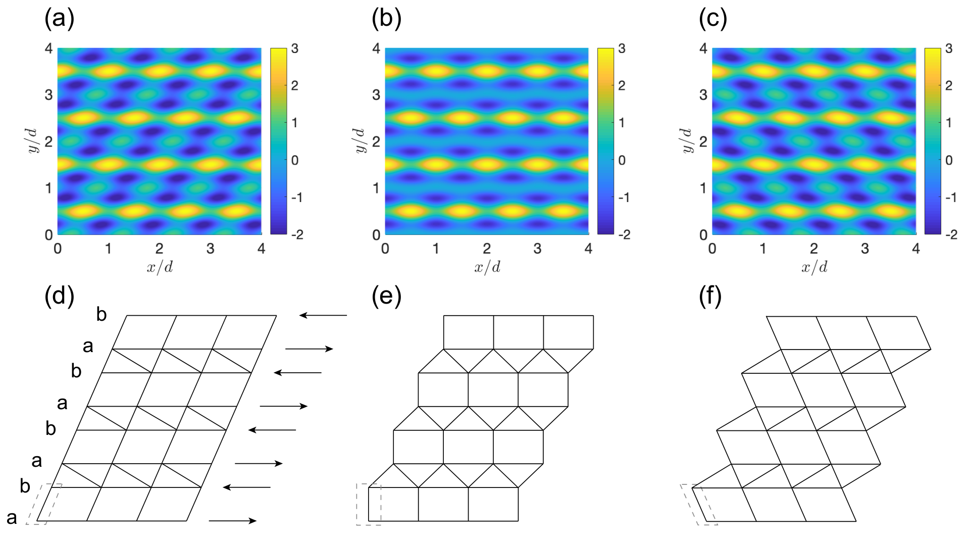
I.2 Positions of the lattice sites

We first derive the time-dependence of the effective lattice site positions by solving for the potential minima. The partial derivatives of the potential $V(x,y)$ give

	$\displaystyle\frac{\partial V(x,y)}{\partial x}$	$\displaystyle=$	$\displaystyle\frac{2\pi\beta}{d}V_{xy}\left[f(\omega_{2}t)\cos\frac{2\pi\beta(x-x_{1})}{d}\cos\frac{\pi y}{d}+\sin\frac{2\pi\beta(x-x_{1})}{d}\sin\frac{\pi y}{d}\right],$
	$\displaystyle\frac{\partial V(x,y)}{\partial y}$	$\displaystyle=$	$\displaystyle\frac{2\pi}{d}V_{y}(1-4\cos\frac{2\pi y}{d})\sin\frac{2\pi y}{d}-\frac{2\pi}{d}\frac{V_{xy}}{2}\left[f(\omega_{2}t)\sin\frac{2\pi\beta(x-x_{1})}{d}\sin\frac{\pi y}{d}+\cos\frac{2\pi\beta(x-x_{1})}{d}\cos\frac{\pi y}{d}\right].$

At oscillation turning points $f(\omega_{2}t)=\pm 1$ , the stationary points of the potential satisfy

	$\displaystyle\pm\cos\frac{2\pi\beta(x-x_{1})}{d}\cos\frac{\pi y}{d}+\sin\frac{2\pi\beta(x-x_{1})}{d}\sin\frac{\pi y}{d}$	$\displaystyle=$	$\displaystyle 0,$
	$\displaystyle\left(1-4\cos\frac{2\pi y}{d}\right)\sin\frac{2\pi y}{d}$	$\displaystyle=$	$\displaystyle 0,$		(S5)

and the minima of $V(x,y)$ are found to be at

	$\displaystyle\frac{2\pi}{d}(x_{0}^{a},y_{0}^{a})_{n_{x},n_{y}}$	$\displaystyle=$	$\displaystyle\left[\frac{2\pi}{d}(x_{1}\pm d_{2}^{a})+(n_{y}-1)\pi+2(n_{x}-1)\pi,\arccos\frac{1}{4}+2(n_{y}-1)\pi\right],$
	$\displaystyle\frac{2\pi}{d}(x_{0}^{b},y_{0}^{b})_{n_{x},n_{y}}$	$\displaystyle=$	$\displaystyle\left[\frac{2\pi}{d}(x_{1}\mp d_{2}^{b})+(n_{y}-1)\pi+2(n_{x}-1)\pi,(2\pi-\arccos\frac{1}{4})+2(n_{y}-1)\pi\right],$		(S6)

with

\displaystyle d_{2}^{a}=-d_{2}^{b}=\frac{d}{4\beta\pi}(\arccos\frac{1}{4}-\pi).

(S7)

When $f(\omega_{2}t)=0$ , the minima of $V(x,y)$ are found to be at

	$\displaystyle\frac{2\pi}{d}(x_{0}^{a},y_{0}^{a})_{n_{x},n_{y}}$	$\displaystyle=$	$\displaystyle\left[\frac{2\pi}{d}x_{1}+(n_{y}-1)\pi+2(n_{x}-1)\pi,\frac{2\pi}{d}d_{y}^{a}+2(n_{y}-1)\pi\right],$
	$\displaystyle\frac{2\pi}{d}(x_{0}^{b},y_{0}^{b})_{n_{x},n_{y}}$	$\displaystyle=$	$\displaystyle\left[\frac{2\pi}{d}x_{1}+(n_{y}-1)\pi+2(n_{x}-1)\pi,\frac{2\pi}{d}d_{y}^{b}+2(n_{y}-1)\pi\right],$		(S8)

with $d_{y}^{a}$ and $d_{y}^{b}$ the first two minima of the potential at $x=0$ and $f(\omega_{2}t)=0$ ,

\displaystyle V(x=0,y)=V_{y}(-\cos\left[\frac{2\pi}{d}y\right]+\cos\left[\frac{4\pi}{d}y\right])-V_{xy}\sin\frac{\pi}{d}y+2V_{y}+V_{xy}.

(S9)

Thus the $f(\omega_{2}t)$ driving induces an oscillation of $y$ -minima with an amplitude of $d_{y,2}=|d_{y}^{a}-\frac{d}{2\pi}\arccos\frac{1}{4}|=|d_{y}^{b}-d+\frac{d}{2\pi}\arccos\frac{1}{4}|$ , and an oscillation of $x$ -minima with an amplitude of $d_{x,2}=\frac{d}{4\beta\pi}(\pi-\arccos\frac{1}{4})$ . We can see that $d_{y,2}$ has a dependence on the ratio of $V_{y}/V_{xy}$ , and is much smaller than $d_{x,2}$ in the parameter region we consider (e.g. $d_{y,2}/d_{x,2}\approx 1/7$ for $V_{xy}=1.5V_{y}$ and $\beta=1$ as chosen for Fig. 2 in main text), hence we shall ignore the shaking along $y$ hereafter, and denote $d_{x,2}$ as $d_{2}$ for simplicity.

The time-dependent position of $x_{0}^{\tau}(t)=x_{1}(t)+x_{2}^{\tau}(t)$ with $\tau\in\{a,b\}$ is given by $\partial V(x,y)/\partial x=0$ , which yields

	$\displaystyle x_{0}^{\tau}$	$\displaystyle=$	$\displaystyle x_{1}+x_{2}^{\tau},$
	$\displaystyle x_{2}^{\tau}$	$\displaystyle=$	$\displaystyle\frac{d}{2\beta\pi}\left[\arctan\left[-f(\omega_{2}t)\cot\left(\frac{\pi y_{0}^{\tau}}{d}\right)\right]+2(n_{x}-1)\pi\right],$		(S10)

with $y_{0}^{\tau}$ the $y$ position of the $\tau$ sublattice. As we have omitted the small shaking along $y$ direction, here we use

\displaystyle\frac{2\pi}{d}y_{0}^{a}=\arccos\frac{1}{4}+2(n_{y}-1)\pi,~~\frac{2\pi}{d}y_{0}^{b}=2\pi-\arccos\frac{1}{4}+2(n_{y}-1)\pi,

(S11)

i. e. the results from Eq. (S6). As in the main text, we choose

\displaystyle f(\omega_{2}t)=A\cos(\omega_{2}t+\varphi),

(S12)

with $\varphi$ a phase factor, and the position shifting of $x_{2}^{\tau}$ has a time period of $2\pi$ . From Eq. (S10) we can also see that $x_{2}^{a}=-x_{2}^{b}$ , which can be represented by a $\pi$ phase difference of the phase factors of the two sublattices, $\varphi_{a}=\varphi_{b}+\pi$ . By choosing $\omega_{2}=2\omega_{1}$ , we can realize the bichromatic tuning Kang et al. with a $\pi$ phase difference between the two sublattices, except that the $f(\omega_{2}t)$ driving corresponds to a position shift described by Eq. S10. The amplitude of the $\omega_{2}$ oscillation can be controlled by tuning $A$ or $\beta$ , resulting in a total amplitude of $d_{2}=\frac{d}{2\beta\pi}\arctan\left[\sqrt{5/3}A\right]$ .

While the actual form of the $\omega_{2}$ oscillation is given by Eq. (S10), it is very similar to a cosine function, especially when $A$ is small, as shown in Fig. S2. In the main text we have considered the case with $d_{2}=d/100$ , corresponding to $A\approx 0.05$ , where the position shifting is almost identical with a cosine function. Therefore, in the following calculations we take $x_{0}^{\tau}=-d_{1}\cos(\omega_{1}t)-d_{2}\cos(\omega_{2}t+\varphi_{\tau})$ with $\varphi_{a}=\varphi_{b}+\pi=\varphi$ , so that we can apply the high frequency approximation to obtain a relatively simple tight-binding model.

Figure S2: Approximation of Eq. (S10) by a single fourier harmonic. The position shifting

x_{2}^{a}

of the first unit cell with different values of

A

. The yellow solid lines are for the actual shifting obtained from Eq. (S10),

x_{2}^{a}=\frac{d}{2\beta\pi}\arctan\left[-\sqrt{5/3}A\cos(\omega_{2}t+\varphi)\right]

, and the black dash lines are for

x_{2}^{a}=-d_{2}\cos(\omega_{2}t+\varphi_{a})

with

d_{2}=\frac{d}{2\beta\pi}\arctan\left[\sqrt{5/3}A\right]

. The shaking of

b

sublattice is given by

x_{2}^{b}=-x_{2}^{a}

. Here we choose the lattice constant to be

d=1

, and

\beta=1

I.3 Effective Hamiltonian

Next we derive the time-dependent Hamiltonian of the above potential. The shaking of the lattice can be effectively described by $x_{0}^{\tau}=-d_{1}\cos(\omega_{1}t)-d_{2}\cos(\omega_{2}t+\varphi_{\tau})$ , and each of the two sublattices corresponds to a series of two-leg ladders with opposite shaking direction of $\omega_{2}$ . The stationary part of the whole 2D system can be given by the potential when each shaking component vanishes, i.e. $f(\omega_{2}t)=0$ and $x_{1}=0$ , with the lattice structure given by Fig. 1(a) in the main text. Thus the static potential is given by

\displaystyle V_{\rm stat}(x,y)=V_{y}(-\cos\left[\frac{2\pi}{d}y\right]+\cos\left[\frac{4\pi}{d}y\right])-V_{xy}\cos\left[\frac{2\pi}{d}\beta x\right]\sin\frac{\pi}{d}y+2V_{y}+V_{xy}.

(S13)

As each lattice site represents a minimum of the potential, we can do the Taylor expansion near it and keep up to the 2nd order term. Due to the translational symmetry, here we consider the two lattice sites of the first unit cell $(n_{x},n_{y})=(1,1)$ as an example. The static lattice position is given by

\displaystyle(x_{0,s}^{a},y_{0,s}^{a})=(0,d_{y}^{a}),~~(x_{0,s}^{b},y_{0,s}^{b})=(0,d_{y}^{b}),

(S14)

where $d_{y}^{a}$ and $d_{y}^{b}$ are the same as Eq. (S8). Near these points the potential can be expanded as

	$\displaystyle\tilde{V}_{\rm stat}(x,y)$	$\displaystyle=$	$\displaystyle V(x_{0,s}^{\tau},y_{0,s}^{\tau})+V_{xy}\frac{2\pi^{2}\beta^{2}}{d^{2}}\sin\left(\frac{\pi}{d}d_{y}^{\tau}\right)x^{2}$		(S15)
			$\displaystyle+\frac{\pi^{2}}{d^{2}}\left[2V_{y}\cos\left(\frac{2\pi}{d}d_{y}^{\tau}\right)-8V_{y}\cos\left(\frac{4\pi}{d}d_{y}^{\tau}\right)+\frac{V_{xy}}{2}\sin\left(\frac{\pi}{d}d_{y}^{\tau}\right)\right](y-d_{y}^{\tau})^{2}.$		(S15)

The corresponding wave-function of $H=\frac{p_{x}^{2}+p_{y}^{2}}{2m}+\tilde{V}_{\rm stat}(x,y)$ takes the same form for the two sublattices, i.e.

\displaystyle\psi_{l_{x},l_{y}}=\sqrt{\frac{1}{2^{l_{x}+l_{y}}l_{x}!l_{y}!}}\left(\frac{m}{\pi\hbar}\right)^{1/2}\left(\omega_{x}\omega_{y}\right)^{1/4}\exp\left[-\frac{m}{2\hbar}(\omega_{x}\delta_{x}^{2}+\omega_{y}\delta_{y}^{2})\right]H_{l_{x}}\left(\sqrt{\frac{m\omega_{x}}{\hbar}}\delta_{x}\right)H_{l_{y}}\left(\sqrt{\frac{m\omega_{y}}{\hbar}}\delta_{y}\right),

(S16)

with $\delta_{x}=x-x_{0,s}^{\tau}$ , $\delta_{y}=y-y_{0,s}^{\tau}$ , $l_{x/y}$ being the quantum numbers of the harmonic oscillators along $x$ and $y$ directions,

\displaystyle H_{l}(z)=(-1)^{l}e^{z^{2}}\frac{d^{n}}{dz^{n}}\left(e^{-z^{2}}\right)

(S17)

the Hermite polynomials, and

	$\displaystyle\omega_{x}$	$\displaystyle=$	$\displaystyle\sqrt{\frac{V_{xy}}{m}\sin\left(\frac{\pi}{d}d_{y}^{\tau}\right)}\frac{2\pi\beta}{d},$
	$\displaystyle\omega_{y}$	$\displaystyle=$	$\displaystyle\frac{2\pi}{d}\sqrt{\frac{1}{m}\left[V_{y}\cos\left(\frac{2\pi}{d}d_{y}^{\tau}\right)-4V_{y}\cos\left(\frac{4\pi}{d}d_{y}^{\tau}\right)+\frac{V_{xy}}{4}\sin\left(\frac{\pi}{d}d_{y}^{\tau}\right)\right]}$		(S18)

the effective frequencies of the oscillators, which take the same values for the two sublattices. The corresponding energy levels are given by

\displaystyle E_{l_{x},l_{y}}=\hbar\left[\omega_{x}(l_{x}+\frac{1}{2})+\omega_{y}(l_{y}+\frac{1}{2})\right]+V(x_{0,s}^{\tau},y_{0,s}^{\tau}).

(S19)

This wave-function approximately gives the Wannier state of the system. Here the $s$ orbital is given by $(l_{x},l_{y})=(0,0)$ , and there are two $p$ orbitals of $p_{x}:~(l_{x},l_{y})=(1,0)$ and $p_{y}:~(l_{x},l_{y})=(0,1)$ . However, as shown later, the inter-orbital couplings are given solely by the periodic shaking, which involves only the first derivative of $x$ . Therefore $p_{y}$ orbital does not couple with the rest two as they involve different $y$ orbitals, and we shall only consider the subspace of $s$ and $p_{x}$ orbital in the following discussion. For simplicity, we shall refer to the $p_{x}$ orbital as $p$ orbital hereafter. Note that in the main text we have labeled the $p$ and $s$ orbitals as pseudopin up and down respectively, to give a simpler picture of the system. In this supplementary material, however, we shall use the language of $p$ and $s$ orbitals, to have a clearer description of how the two orbitals interact with each other under the periodic shaking.

With the above wave-function, we can now calculate the coupling strengths and construct a tight-binding model of the system. While we consider a 2D system, the shaking of the lattice positions is mostly along $x$ -direction for the parameters we choose, making the lattice structure along $y$ -direction irrelevant to the shaking-induced inter-orbital couplings. This is because this shaking only induces a $x$ -momentum term to the Hamiltonian, which commutes with the $y$ -component of the Wannier state. Since the coupling strength is given by the overlap integral of the Wannier states and the Hamiltonian, the $y$ -component shall only give a coefficient of unity to this term if the Wannier states are of the same $y$ -orbital at the same $y$ -position, and $0$ otherwise. Therefore, as the total position shaking $x_{0}^{\tau}$ has a dependence on the sublattice index $\tau\in\{a,b\}$ , we can use different effective Hamiltonians $H^{\tau}$ for the two sublattices to determine the shaking-induced couplings,

\displaystyle H^{\tau}=\frac{p_{x}^{2}+p_{y}^{2}}{2m}+V_{y}\left(-\cos\left[\frac{2\pi}{d}y\right]+\cos\left[\frac{4\pi}{d}y\right]\right)-V_{xy}\sin\left[\frac{\pi}{d}y\right]\cos\left[\frac{2\pi}{d}\beta[x-x_{0}^{\tau}(t)]\right]+2V_{y}+V_{xy}.

(S20)

By transforming to the co-moving frame Mei et al. 2014; Zheng and Zhai 2014; Kang et al., $x\rightarrow x+x_{0}^{\tau}(t)$ , the Hamiltonians becomes $H^{\tau}=H_{\rm stat}+\delta H^{\tau}(t)$ with the same stationary part given by

\displaystyle H_{\rm stat}

\displaystyle=

\displaystyle\frac{p_{x}^{2}+p_{y}^{2}}{2m}+V_{y}\left(-\cos\left[\frac{2\pi}{d}y\right]+\cos\left[\frac{4\pi}{d}y\right]\right)-V_{xy}\sin\left[\frac{\pi}{d}y\right]\cos\left[\frac{2\pi}{d}\beta x\right]+2V_{y}+V_{xy},

(S21)

which is consistent with the the stationary part of the original potential, given by Eq. (S13). The time-dependent terms are given by

\displaystyle\delta H^{\tau}(t)

\displaystyle=

\displaystyle-\omega_{1}d_{1}\sin(\omega_{1}t)p_{x}-\omega_{2}d_{2}\sin(\omega_{2}t+\varphi_{\tau})p_{x}.

(S22)

Thus the tight-binding Hamiltonian is given by

	$\displaystyle H_{\rm TB}$	$\displaystyle=$	$\displaystyle\sum_{n_{x},n_{y}}\sum_{\tau=a,b}\{\Psi^{\dagger}_{\tau,{n_{x},n_{y}}}K_{\tau}(t)\Psi_{\tau,{n_{x},n_{y}}}-[\Psi^{\dagger}_{\tau,{n_{x},n_{y}}}J_{x,\tau}(t)\Psi_{\tau,{n_{x},n_{y}}+1}+H.c.]\}$		(S23)
			$\displaystyle-\sum_{n_{x},n_{y}}[\Psi^{\dagger}_{a,{n_{x},n_{y}}}J_{y}(t)\Psi_{b,{n_{x},n_{y}}}+\Psi^{\dagger}_{b,{n_{x},n_{y}}}J^{\prime}_{y,+}(t)\Psi_{a,{n_{x},n_{y}+1}}+\Psi^{\dagger}_{b,{n_{x},n_{y}}}J^{\prime}_{y,-}(t)\Psi_{a,{n_{x}-1,n_{y}+1}}+H.c.],$		(S23)

where $\Psi^{\dagger}_{\tau,{n_{x},n_{y}}}=(\hat{\tau}^{\dagger}_{{n_{x},n_{y}},p},\hat{\tau}^{\dagger}_{{n_{x},n_{y}},s})$ , $\hat{\tau}^{\dagger}_{j,\sigma}$ with $\hat{\tau}\in\{\hat{a},\hat{b}\}$ is the creation operator for the atom on lattice site $(n_{x},n_{y})$ in orbital $\sigma\in\{p,s\}$ , $s$ and $p$ correspond to the orbitals of $(l_{x},l_{y})=(0,0)$ and $(1,0)$ respectively. The $K$ and $J$ matrices $K(t)$ are given by

$\displaystyle K_{\tau}(t)$	$\displaystyle=$	$\displaystyle\left(\begin{matrix}\epsilon_{p}&-i[h_{0}^{sp}\sin(\omega_{1}t)+\tilde{h}_{0}^{sp}\sin(\omega_{2}t+\varphi_{\tau})]\\ i[h_{0}^{sp}\sin(\omega_{1}t)+\tilde{h}_{0}^{sp}\sin(\omega_{2}t+\varphi_{\tau})]&\epsilon_{s}\end{matrix}\right),$
$\displaystyle J_{x,\tau}(t)$	$\displaystyle=$	$\displaystyle\left(\begin{matrix}t_{p}-i[h_{1}^{pp}\sin(\omega_{1}t)+\tilde{h}_{1}^{pp}\sin(\omega_{2}t+\varphi_{\tau})]&i[h_{1}^{sp}\sin(\omega_{1}t)+\tilde{h}_{1}^{sp}\sin(\omega_{2}t+\varphi_{\tau})]\\ -i[h_{1}^{sp}\sin(\omega_{1}t)+\tilde{h}_{1}^{sp}\sin(\omega_{2}t+\varphi_{\tau})]&t_{s}-i[h_{1}^{ss}\sin(\omega_{1}t)+\tilde{h}_{1}^{ss}\sin(\omega_{2}t+\varphi_{\tau})]\end{matrix}\right),$
$\displaystyle J_{y}$	$\displaystyle=$	$\displaystyle\left(\begin{matrix}t_{p}^{\rm intra}&0\\ 0&t_{s}^{\rm intra}\end{matrix}\right),~~J^{\prime}_{y,\pm}=\left(\begin{matrix}t_{p,\pm}^{\rm inter}&0\\ 0&t_{s,\pm}^{\rm inter}.\end{matrix}\right),$	(S24)

with

$\displaystyle\epsilon_{\sigma}$	$\displaystyle=$	$\displaystyle\int\int dxdy\psi_{\sigma}(x,y-y_{0}^{\tau})H_{\rm stat}\psi_{\sigma}(x,y-y_{0}^{\tau}),$
$\displaystyle t_{\sigma}$	$\displaystyle=$	$\displaystyle-\int\int dxdy\psi_{\sigma}(x,y-y_{0}^{\tau})H_{\rm stat}\psi_{\sigma}(x-\frac{d}{\beta},y-y_{0}^{\tau}),$
$\displaystyle h_{l}^{\sigma\sigma^{\prime}}$	$\displaystyle=$	$\displaystyle\hbar\omega_{1}d_{1}\int\int dxdy\psi_{\sigma}(x,y-y_{0}^{\tau}){\partial_{x}}\psi_{\sigma^{\prime}}(x-\frac{ld}{\beta},y-y_{0}^{\tau}),$
$\displaystyle\tilde{h}_{l}^{\sigma\sigma^{\prime}}$	$\displaystyle=$	$\displaystyle\hbar\omega_{2}d_{2}\int\int dxdy\psi_{\sigma}(x,y-y_{0}^{\tau}){\partial_{x}}\psi_{\sigma^{\prime}}(x-\frac{ld}{\beta},y-y_{0}^{\tau}),$
$\displaystyle t^{\rm intra}_{\sigma}$	$\displaystyle=$	$\displaystyle-\int\int dxdy\psi_{\sigma}(x,y-y_{0}^{a})H_{\rm stat}\psi_{\sigma}(x,y-y_{0}^{b}),$
$\displaystyle t^{\rm inter}_{\sigma,\pm}$	$\displaystyle=$	$\displaystyle-\int\int dxdy\psi_{\sigma}(x,y-y_{0}^{b})H_{{\rm stat}}\psi_{\sigma}(x\mp\frac{d}{2\beta},y-y_{0}^{a}-d).$	(S25)

Here $\phi_{\sigma}$ is given by $\psi_{l_{x},l_{y}}$ with $(l_{x},l_{y})=(1,0)$ [ $(0,0)$ ] for $\sigma=p$ ( $s$ ), and each of the first four integrals takes the same value for $\tau=a$ or $b$ .

The tight-binding Hamiltonian can be written in terms of two sets of Pauli matrices and identity matrices, $\sigma_{i}$ and $\tau_{i}$ with $i=0,1,2,3$ , acting on the $sp$ -orbital space and the $ab$ -sublattice space respectively. Here we rewrite the Hamiltonian in momentum space, i.e.

\displaystyle H_{\rm TB}(\bm{k})=\sum_{\bm{k}}\Psi^{\dagger}_{\bm{k}}h_{\rm TB}(\bm{k})\Psi_{\bm{k}}

(S26)

with $\Psi^{\dagger}_{\bm{k}}=(\hat{a}_{p,{\bm{k}}},\hat{a}_{s,{\bm{k}}},\hat{b}_{p,{\bm{k}}},\hat{b}_{s,{\bm{k}}})$ , and

$\displaystyle h_{\rm TB}(k_{x},k_{y})$	$\displaystyle=$	$\displaystyle\left[\bar{\epsilon}-2t_{+,x}\cos k_{x}-2h_{1,+}^{x}\sin k_{x}\sin(\omega_{1}t)\right]\sigma_{0}\tau_{0}-2\tilde{h}_{1,+}^{x}\sin k_{x}\sin(\omega_{2}t+\varphi)\sigma_{0}\tau_{3}$	(S27)
		$\displaystyle+\left[\frac{\epsilon_{sp}}{2}-2t_{-,x}\cos k_{x}-2h_{1,-}^{x}\sin k_{x}\sin(\omega_{1}t)\right]\sigma_{3}\tau_{0}-2\tilde{h}_{1,-}^{x}\sin k_{x}\sin(\omega_{2}t+\varphi)\sigma_{3}\tau_{3}$
		$\displaystyle+\left[h_{0}^{sp}\sin(\omega_{1}t)+2h_{1}^{sp}\cos k_{x}\sin(\omega_{1}t)\right]\sigma_{2}\tau_{0}+\left[\tilde{h}_{0}^{sp}\sin(\omega_{2}t+\varphi)+2\tilde{h}_{1}^{sp}\cos k_{x}\sin(\omega_{2}t+\varphi)\right]\sigma_{2}\tau_{3}$
		$\displaystyle-\{t_{+,y}+t^{\prime}_{+,y}\left[\cos k_{y}+\cos(k_{y}-k_{x})\right]\}\sigma_{0}\tau_{1}-t^{\prime}_{+,y}\left[\sin k_{y}+\sin(k_{y}-k_{x})\right]\sigma_{0}\tau_{2}$
		$\displaystyle-\{t_{-,y}+t^{\prime}_{-,y}\left[\cos k_{y}+\cos(k_{y}-k_{x})\right]\}\sigma_{3}\tau_{1}-t^{\prime}_{-,y}\left[\sin k_{y}+\sin(k_{y}-k_{x})\right]\sigma_{3}\tau_{2},$

with

	$\displaystyle\bar{\epsilon}=\frac{\epsilon_{p}+\epsilon_{s}}{2},~~\epsilon_{sp}=\epsilon_{p}-\epsilon_{s},$
	$\displaystyle t_{\pm,x}=\frac{t_{p}\pm t_{s}}{2},~~t_{\pm,y}=\frac{t^{\rm intra}_{p}\pm t^{\rm intra}_{s}}{2},~~t^{\prime}_{\pm,y}=\frac{t^{\rm inter}_{p}\pm t^{\rm inter}_{s}}{2},$
	$\displaystyle h^{x}_{1,\pm}=\frac{h_{1}^{pp}\pm h_{1}^{ss}}{2},~~\tilde{h}^{x}_{1,\pm}=\frac{\tilde{h}_{1}^{pp}\pm\tilde{h}_{1}^{ss}}{2}.$

Finally, following Ref. Kang et al., we consider the effects of the photon-assisted inter-orbital resonant coupling, and obtain the Hamiltonian in a rotating reference frame with frequency $\omega_{2}=2\omega_{1}$ , taking a unitary transformation of

\displaystyle U(t)=\cos(\frac{\omega_{2}}{2}t)\sigma_{0}\tau_{0}-i\sin(\frac{\omega_{2}}{2}t)\sigma_{3}\tau_{0}.

(S28)

The final Hamiltonian takes the form of

$\displaystyle h^{\prime}_{\rm TB}(k_{x},k_{y})$	$\displaystyle=$	$\displaystyle\left[\bar{\epsilon}-2t_{+,x}\cos k_{x}-2h_{1,+}^{x}\sin k_{x}\sin(\omega_{1}t)\right]\sigma_{0}\tau_{0}-2\tilde{h}_{1,+}^{x}\sin k_{x}\sin(\omega_{2}t+\varphi)\sigma_{0}\tau_{3}$	(S29)
		$\displaystyle+\left[(\epsilon_{sp}-\hbar\omega_{2})/2-2t_{-,x}\cos k_{x}-2h_{1,-}^{x}\sin k_{x}\sin(\omega_{1}t)\right]\sigma_{3}\tau_{0}-2\tilde{h}_{1,-}^{x}\sin k_{x}\sin(\omega_{2}t+\varphi)\sigma_{3}\tau_{3}$
		$\displaystyle+\cos(\omega_{2}t)\left[h_{0}^{sp}\sin(\omega_{1}t)+2h_{1}^{sp}\cos k_{x}\sin(\omega_{1}t)\right]\sigma_{2}\tau_{0}+\cos(\omega_{2}t)\left[\tilde{h}_{0}^{sp}\sin(\omega_{2}t+\varphi)+2\tilde{h}_{1}^{sp}\cos k_{x}\sin(\omega_{2}t+\varphi)\right]\sigma_{2}\tau_{3}$
		$\displaystyle+\sin(\omega_{2}t)\left[h_{0}^{sp}\sin(\omega_{1}t)+2h_{1}^{sp}\cos k_{x}\sin(\omega_{1}t)\right]\sigma_{1}\tau_{0}+\sin(\omega_{2}t)\left[\tilde{h}_{0}^{sp}\sin(\omega_{2}t+\varphi)+2\tilde{h}_{1}^{sp}\cos k_{x}\sin(\omega_{2}t+\varphi)\right]\sigma_{1}\tau_{3}$
		$\displaystyle-\{t_{+,y}+t^{\prime}_{+,y}\left[\cos k_{y}+\cos(k_{y}-k_{x})\right]\}\sigma_{0}\tau_{1}-t^{\prime}_{+,y}\left[\sin k_{y}+\sin(k_{y}-k_{x})\right]\sigma_{0}\tau_{2}$
		$\displaystyle-\{t_{-,y}+t^{\prime}_{-,y}\left[\cos k_{y}+\cos(k_{y}-k_{x})\right]\}\sigma_{3}\tau_{1}-t^{\prime}_{-,y}\left[\sin k_{y}+\sin(k_{y}-k_{x})\right]\sigma_{3}\tau_{2}.$

Next we consider the high frequency regime of the oscillation, where the effective Floquet Hamiltonian can be given by the Magnus expansion approximation,

\displaystyle h_{\rm eff}=h_{0}+\sum_{n=1}^{\infty}\frac{[h_{n},h_{-n}]}{n\hbar\omega_{1}},

(S30)

where $h_{n}$ is the $n$ th Fourier component of $h^{\prime}_{\rm TB}(\bm{k})$ , i.e.

\displaystyle h^{\prime}_{\rm TB}=\sum_{n}h_{n}e^{in\omega_{1}t}.

(S31)

Specifically, we have

$\displaystyle h_{0}$	$\displaystyle=$	$\displaystyle\left[\bar{\epsilon}-2t_{+,x}\cos k_{x}\right]\sigma_{0}\tau_{0}+\left[(\epsilon_{sp}-\hbar\omega_{2})/2-2t_{-,x}\cos k_{x}\right]\sigma_{3}\tau_{0}$
		$\displaystyle+\frac{1}{2}(\tilde{h}_{0}^{sp}+2\tilde{h}_{1}^{sp}\cos k_{x})\left[\sin(\varphi)\sigma_{2}+\cos(\varphi)\sigma_{1}\right]\tau_{3}$
		$\displaystyle-\{t_{+,y}+t^{\prime}_{+,y}\left[\cos k_{y}+\cos(k_{y}-k_{x})\right]\}\sigma_{0}\tau_{1}-t^{\prime}_{+,y}\left[\sin k_{y}+\sin(k_{y}-k_{x})\right]\sigma_{0}\tau_{2}$
		$\displaystyle-\{t_{-,y}+t^{\prime}_{-,y}\left[\cos k_{y}+\cos(k_{y}-k_{x})\right]\}\sigma_{3}\tau_{1}-t^{\prime}_{-,y}\left[\sin k_{y}+\sin(k_{y}-k_{x})\right]\sigma_{3}\tau_{2},$
$\displaystyle h_{1}$	$\displaystyle=$	$\displaystyle ih_{1,+}^{x}\sin k_{x}\sigma_{0}\tau_{0}+ih_{1,-}^{x}\sin k_{x}\sigma_{3}\tau_{0}+\frac{1}{4}(h_{0}^{sp}+2h_{1}^{sp}\cos k_{x})(\sigma_{1}+i\sigma_{2})\tau_{0}$
$\displaystyle h_{2}$	$\displaystyle=$	$\displaystyle i\tilde{h}^{x}_{1,+}\sin k_{x}e^{i\varphi}\sigma_{0}\tau_{3}+i\tilde{h}^{x}_{1,-}\sin k_{x}e^{i\varphi}\sigma_{3}\tau_{3}$
$\displaystyle h_{3}$	$\displaystyle=$	$\displaystyle-\frac{1}{4}(h_{0}^{sp}+2h_{1}^{sp}\cos k_{x})(\sigma_{1}+i\sigma_{2})\tau_{0}$
$\displaystyle h_{4}$	$\displaystyle=$	$\displaystyle-\frac{1}{4}(\tilde{h}_{0}^{sp}+2\tilde{h}_{1}^{sp}\cos k_{x})e^{i\varphi}(\sigma_{1}+i\sigma_{2})\tau_{3},$	(S32)

and $h_{-n}=h_{n}^{\dagger}$ . Thus the effective Hamiltonian is given by

$\displaystyle h_{\rm eff}$	$\displaystyle=$	$\displaystyle h_{0}-\frac{h_{1,-}^{x}h_{0}^{sp}\sin(k_{x})+h_{1,-}^{x}h_{1}^{sp}\sin(2k_{x})}{\hbar\omega_{1}}\sigma_{2}\tau_{0}$	(S33)
		$\displaystyle+\frac{(h_{0}^{sp})^{2}+4h_{0}^{sp}h_{1}^{sp}\cos(k_{x})+2(h_{1}^{sp})^{2}+2(h_{1}^{sp})^{2}\cos(2k_{x})}{3\hbar\omega_{1}}\sigma_{3}\tau_{0}$
		$\displaystyle+\frac{(\tilde{h}_{0}^{sp})^{2}+4\tilde{h}_{0}^{sp}\tilde{h}_{1}^{sp}\cos(k_{x})+2(\tilde{h}_{1}^{sp})^{2}+2(\tilde{h}_{1}^{sp})^{2}\cos(2k_{x})}{16\hbar\omega_{1}}\sigma_{3}\tau_{3}.$

With $\hbar\omega_{1}>h_{0}^{sp}\gg h_{1}^{sp}$ , and $h_{l}^{\sigma\sigma^{\prime}}\gg\tilde{h}_{l}^{\sigma\sigma^{\prime}}$ (providing $d_{1}\gg d_{2}$ ), the Hamiltonian is approximated as

$\displaystyle h_{\rm eff}$	$\displaystyle\approx$	$\displaystyle\left[\Delta_{+}-2t_{+,x}\cos k_{x}\right]\sigma_{0}\tau_{0}+\left[\Delta_{-}-2(t_{-,x}-\frac{2h_{0}^{sp}h_{1}^{sp}}{3\hbar\omega_{1}})\cos k_{x}\right]\sigma_{3}\tau_{0}$	(S34)
		$\displaystyle+t_{v}\cos k_{x}\left[\sin(\varphi)\sigma_{2}+\cos(\varphi)\sigma_{1}\right]\tau_{3}-2t_{d}\sin(k_{x})\sigma_{2}\tau_{0}$
		$\displaystyle-\{t_{+,y}+t^{\prime}_{+,y}\left[\cos k_{y}+\cos(k_{y}-k_{x})\right]\}\sigma_{0}\tau_{1}-t^{\prime}_{+,y}\left[\sin k_{y}+\sin(k_{y}-k_{x})\right]\sigma_{0}\tau_{2}$
		$\displaystyle-\{t_{-,y}+t^{\prime}_{-,y}\left[\cos k_{y}+\cos(k_{y}-k_{x})\right]\}\sigma_{3}\tau_{1}-t^{\prime}_{-,y}\left[\sin k_{y}+\sin(k_{y}-k_{x})\right]\sigma_{3}\tau_{2},$

with

	$\displaystyle\Delta_{+}=\bar{\epsilon},~~\Delta_{-}=(\epsilon_{sp}-2\hbar\omega_{1})/2+\frac{(h_{0}^{sp})^{2}}{3\hbar\omega_{1}},$
	$\displaystyle t_{v}=\frac{1}{2}\tilde{h}_{0}^{sp},~~t_{d}=\frac{h_{1,-}^{x}h_{0}^{sp}}{2\hbar\omega_{1}}.$

Note the here the term $\frac{2h_{0}^{sp}h_{1}^{sp}}{3\hbar\omega_{1}}$ is added to $t_{-,x}$ , thus it also contributes to the intra-orbital couplings of $t_{p}$ and $t_{s}$ along $x$ direction. The parameters $t_{\uparrow,x}$ , $t_{\downarrow,x}$ , and $t_{-,x}$ in the main text are given by $t_{p}-\frac{2h_{0}^{sp}h_{1}^{sp}}{3\hbar\omega_{1}}$ , $t_{s}+\frac{2h_{0}^{sp}h_{1}^{sp}}{3\hbar\omega_{1}}$ , and $t_{-,x}-\frac{2h_{0}^{sp}h_{1}^{sp}}{3\hbar\omega_{1}}$ of the above discussion respectively. Finally, we note that when $V_{y}$ is much larger than $V_{xy}$ , the couplings along $y$ -direction become extremely weak, and the 2D model reduces to a series of decoupled 1D chains analogous to that of Ref. Kang et al..

II Edge states with inter-orbital couplings and atom loss

Here we elaborate on the Gedanken experiment of tuning the inter-sublattice couplings, as introduced in the main text. When the shaking frequencies $\omega_{1}=\omega_{2}=0$ , the two orbitals are decoupled, resulting in two $2\times 2$ subsystems described by

\displaystyle h_{p}(\bm{k})=-(2t_{p,x}\cos k_{x}-\epsilon_{p})\tau_{0}-\{t_{p,y}+t^{\prime}_{p,y}\left[\cos k_{y}+\cos(k_{y}-k_{x})\right]\}\tau_{1}-t^{\prime}_{p,y}\left[\sin k_{y}+\sin(k_{y}-k_{x})\right]\tau_{2}

(S35)

and

\displaystyle h_{s}(\bm{k})=-(2t_{s,x}\cos k_{x}-\epsilon_{s}+2ig)\tau_{0}-\{t_{s,y}+t^{\prime}_{s,y}\left[\cos k_{y}+\cos(k_{y}-k_{x})\right]\}\tau_{1}-t^{\prime}_{s,y}\left[\sin k_{y}+\sin(k_{y}-k_{x})\right]\tau_{2}

(S36)

for the two orbitals respectively, each of which possesses a 1D $Z$ -type topology due to the absence of the third Pauli matrix $\tau_{3}$ . Consequently, under $x$ -PBC/ $y$ -OBC, the system shall have a pair of degenerate edge modes for each subsystem in a certain range of $k_{x}$ , as shown in Fig. S3(a). The high-frequency shaking we consider couples the two orbitals through the photon-assisted inter-orbital resonant couplings and mixes the energy bands of the two orbitals, as shown in Fig. S3(b). On the other hand, by comparing Figs. S3(a) and (b), we can see that the region of $k_{x}$ that hosts 1D edge modes remains roughly unchanged, except for some $k_{x}$ the edge modes overlap with the bulk bands, due to the mixing of the bands. Therefore we can still use the Berry phase for this decoupled scenario to characterize the edge modes under nonzero frequencies $\omega_{1}$ and $\omega_{2}$ .

By introducing atom loss to the $s$ orbital, the two pairs of energy bands, mainly given by the two orbitals respectively, acquire different imaginary energies and thus possess an imaginary gap, as shown in Fig. (S3)(c,d). The edge modes are now once again fully separated from the bulk bands, while their existence is almost not affected.

III Non-Hermitian skin effect of the effective 1D Hamiltonian of the two-leg ladder along $x$ direction

As discussed in the main text, when tuning off the coupling along $y$ direction, the 2D system we consider can be viewed as a series of two-leg ladders of the two sublattices $a$ and $b$ . For each sublattice $\tau=a,b$ , the effective 1D Hamiltonian is $H_{\rm 1D}^{\tau,x}=\sum_{k_{x}}\hat{\Psi}^{\dagger}_{\tau,k_{x}}h_{\rm 1D}^{\tau,x}({k_{x}})\hat{\Psi}_{\tau,k_{x}}$ , with

$\displaystyle h_{\rm 1D}^{\tau,x}({k_{x}})$	$\displaystyle=$	$\displaystyle-(2t_{+,x}\cos{k_{x}}+ig)\sigma_{0}+(t_{v}\cos\varphi_{\tau})\sigma_{1}$	(S37)
		$\displaystyle+(t_{v}\sin\varphi_{\tau}+2t_{d}\sin{k_{x}})\sigma_{2}$
		$\displaystyle-(2t_{-,x}\cos{k_{x}}-\Delta_{-}-ig)\sigma_{3},$

with $\hat{\Psi}^{\dagger}_{\tau,k_{x}}=(\hat{\tau}^{\dagger}_{\uparrow,k_{x}},\hat{\tau}^{\dagger}_{\downarrow,k_{x}})$ , and $\varphi_{a}=\varphi_{b}+\pi=\varphi$ . In the simplest case of $\varphi=\pi/2$ , the system possesses only two of the three Pauli matrices, and is exactly equivalent to the Su-Schrieffer-Heeger (SSH) model Su et al. 1979 upon a basis rotation $\sigma_{3}\rightarrow\sigma_{2}\rightarrow\sigma_{1}\rightarrow\sigma_{3}$ and a $\pi/2$ shift of the quasi-momentum $k_{x}$ . With this rotation, the non-Hermitian term of $ig\sigma_{3}$ in Eq. S37 is transformed into the usual non-reciprocal coupling $ig\sigma_{2}$ for the SSH model, which is associated with the NHSE Yao and Wang 2018. Through such basis rotations, we can show that the NHSE generically occurs whenever non-Hermiticity and TR breaking are simultaneously present, even if not within the same coupling, as in dissipative on-site mechanisms on a TR-broken lattice Song et al. 2019b.

The eigenenergies of the effective 1D Hamiltonian are given by

\displaystyle E^{\tau}_{\pm}(k_{x})=-(2t_{+,x}\cos{k_{x}}+ig)\pm\sqrt{f_{0}+f_{1}(k_{x})+f^{\tau}_{2}(k_{x})},

(S38)

with

$\displaystyle f_{0}$	$\displaystyle=$	$\displaystyle t_{v}^{2}+\Delta_{-}^{2}-g^{2}+2i\Delta_{-}g,$
$\displaystyle f_{1}(k_{x})$	$\displaystyle=$	$\displaystyle 4t_{d}^{2}\sin^{2}k_{x}+4t^{2}_{-,x}\cos^{2}k_{x}-4\Delta_{-}t_{-,x}\cos k_{x}-4it_{-,x}g\cos k_{x},$
$\displaystyle f_{2}^{\tau}(k_{x})$	$\displaystyle=$	$\displaystyle 4t_{v}t_{d}\sin\varphi_{\tau}\sin k_{x}.$	(S39)

The non-Hermitian skin effect (NHSE) in this system can be described by a non-Bloch variation of the Hamiltonian, $H(k+i\kappa_{x})$ , which recovers the OBC spectrum (exact for possible topological edge states), and the imaginary flux $\kappa_{x}$ has an correspondence to the inverse localization length of the skin localization Lee and Thomale 2019; Lee et al. 2019; Li et al. 2019b. In our model, we can see that the eigenenergies satisfy

\displaystyle E^{a}_{\pm}(k_{x}+i\kappa_{x})=E^{b}_{\pm}(-k_{x}-i\kappa_{x}),

(S40)

which suggests that the two-leg ladders of the two sublattices correspond to opposite skin-localization lengths, i.e. opposite directions of the nonreciprocal pumping.

IV reflection of the non-reciprocal pumping in a finite-size system

In a finite-size system, the non-reciprocal pumping along $x$ direction of a prepared state will eventually reach the boundary of the system. Unlike 2D topological chiral edge states which circularly move along the 1D boundaries, the motion of a wavepacket in our system is governed by a different mechanism and will be reflected when hitting the boundary. The wavepacket shall move towards the opposite direction hereafter, and hence suffers a different decaying rate.

In Fig. S4(a,b), we illustrate the spatial densities at different evolution time for $\Psi^{L/R}$ defined in the main text. As we can see, in both cases the prepared states hit the other ends of the system at $\sim 4$ ms. After that, the wavepacket begins to move toward the opposite direction, which can be see from its average $x$ position shown in Fig. S4(e). In Fig. S4(c,d) we demonstrate the population distributions $n(t)$ of the two cases, and their time derivatives. We can see that $\Psi^{R}$ decays faster after $\sim 4$ ms as it now moves against the non-reciprocal pumping direction [pink arrows in panel (a,b)]. On the other hand, in contrast to $\Psi_{R}$ , the decaying rate of $\Psi^{L}$ does not change dramatically for the same evolution time. This is because both of $\Psi^{L/R}$ also slowly diffuse into the bulk in the evolution, and since $\Psi^{L}$ decays faster at the boundary, its diffusion is more dominated. As in our system the non-reciprocal pumping is only along the boundaries, a wavepacket diffused into the bulk is no longer governed by this mechanism.

V Second-order topological phases of the 2D lattice without dissipation.

Here we discuss the connection between our setup and second-order topological corner modes, which also appear in a geometrically similar lattice. Such second-order modes, which are not the focus of our work, can only be mathematically realized by extending the parameters of our setup to physically not-so-realistic values.

In our construction, the effective two-leg ladders within each sublattice are analogs of the SSH model at $\varphi=\pm\pi/2$ , hence they possess 1D Z-type topology and support topological edge localization also along the $x$ direction. These topological edge modes cannot induce non-reciprocal pumping along $y$ direction, as the atom loss considered here does not induce to NHSE along that direction. However, the combination of topological edge localizations along the $x$ and $y$ directions can lead to 2nd-order topological corner modes Benalcazar et al. 2017a; Benalcazar et al. 2017b; Li et al. 2018b in an extended parameter range, as shown in Fig. S5. The existence of these 2nd-order topological corner modes in Fig. S5(a) is protected by the band gap at the zero energy.

Topology-Induced Spontaneous Non-reciprocal Pumping in Cold-Atom Systems with Loss

Abstract

Acknowledgements.

References

I Derivation of the 2D tight-binding model

I.1 The lattice potential

I.2 Positions of the lattice sites

I.3 Effective Hamiltonian

II Edge states with inter-orbital couplings and atom loss

III Non-Hermitian skin effect of the effective 1D Hamiltonian of the two-leg ladder along xx direction

IV reflection of the non-reciprocal pumping in a finite-size system

V Second-order topological phases of the 2D lattice without dissipation.

III Non-Hermitian skin effect of the effective 1D Hamiltonian of the two-leg ladder along $x$ direction