Spaces of Geodesic Triangulations of SurfacesThanks: The author was supported in part by NSF Grant DMS-1719582.

Given a triangulation $T=(V,E,F)$ of the 2-disk with vertices $V$, edges $E$ and faces $F$, the $1$-skeleton of $T$ is a planar graph. Tutte [22] provided a constructive method to generate a straight-line embedding of a 3-vertex-connected planar graph shown in Figure 2. The procedure starts by setting one face of the graph as a convex polygon, then solves for the coordinates of the other vertices with a system of linear equations.

Using a discrete maximum principle, Floater [12] extended Tutte’s result for the case of triangulations of the 2-disk.

Theorem 2.1 is a discrete version of the Rado-Kneser-Choquet theorem [11], which states that a smooth harmonic map from the unit 2-disk to a convex domain bounded by a Jordan curve in the plane is homeomorphic, when its restriction to the boundary of the 2-disk is homeomorphic. Moreover, it gives a constructive method to produce geodesic triangulations of a convex polygon with the combinatorial type of $T$ as follows.

Step 1. Assign a positive weight $c_{ij}$ to a directed edge $(i,j)\in\vec{E}$, where $\vec{E}$ is the set of directed edges of $T$. Then normalize the weights to make the sum of all outgoing weights around each interior vertex equal to $1$

The set $N(v_{i})$ consists of all the vertices that are neighbors of the vertex $v_{i}\in V_{I}$. Notice that we don’t impose symmetry condition $w_{ij}=w_{ji}$.

Step 2. Fix the coordinates of boundary vertices $V_{B}$, which together form a convex $n$-sided polygon $\Omega$,

The coordinates of vertices in $V_{B}$ are determined by the map $\phi$.

Step 3. Solve the coordinates for interior vertices with boundary coordinates given by Step 2,

Step 4. Put the vertices in the positions given by these coordinates, and connect the vertices with line segments based on the combinatorics of the triangulation $T$.

Theorem 2.1 states that the result is a geodesic triangulation of $\Omega$ with the combinatorial type of $T$. The linear system in Step 3 implies that the $x$-coordinate (or $y$-coordinate) of one interior vertex is a convex combination of the $x$-coordinates (or $y$-coordinates) of its neighbors. The coefficient matrix of this system is not necessarily symmetric but it is diagonally dominant, so the solution exists and is unique. This procedure is called Tutte’s method.

This method has been generalized to surfaces with non-trivial topologies. Colin de Verdiere [10] and Hass and Scott [16] showed that every triangulation of a closed surface with a metric of non-positive curvature can be realized as a geodesic triangulation. Gortler, Gotsman, and Thurston [15] reproved Tutte’s theorem using discrete one forms and generalized it to the cases of flat tori and multiple-connected polygonal regions, with appropriate assumptions on the boundaries. Aigerman and Lipman [1] further extended this method to Euclidean orbifolds with spherical topology.

The building block is the polygon $\mathcal{P}$ in the Figure 4. The triangulation $T$ of $\mathcal{P}$ is given in Figure 4 with three interior vertices $P$, $L$, and $R$. For simplicity, in the remaining part of this paper, we only draw a part of the triangulation shown in Figure 4(B) instead of the full triangulation shown in Figure 4(A). Notice that we can add edges back to produce the full triangulation, once the positions of the interior vertices are fixed.

Set $c=(2+\sqrt{2})/(3+\sqrt{2})$. The coordinates of boundary vertices of $\mathcal{P}$ are

Reflect the vertices $A$, $B$, $C$, and $D$ about $y$-axis to determine the remaining boundary vertices $A^{\prime}$, $B^{\prime}$, $C^{\prime}$, and $D^{\prime}$.

The idea of the construction of $\mathcal{P}$ originates from the example given by Bing and Starbird [3]. Let us consider an isosceles wedge $\angle A^{\prime}KA$ in Figure 5 defined by

Let the vertex $P=(t,kt-k)$ move along the edge $KA$ for $t\in(0,1)$. The lines $PB$ and $PB^{\prime}$ are

Set $R$ as the intersection of $PB$ with $x=c$, and $L$ as the intersection of $PB^{\prime}$ with $x=-c$. The line $LR$ is given by

The $y$-intercept $H$ of $LR$ is

Note that the function $h(t,k)$ is not a monotonic function of $t$, but a monotonic decreasing function of $k$. The maximum of $h(t,k)$ in $0\leq t\leq c$ given below, denoted as $\mathbf{h}(k)$, is a continuous monotonically decreasing function of $k$

This corresponds to a clear geometric interpretation: if $k$ increases, the vertex $K$ moves downward, then the vertex $L$ and $R$ moves downward, so $\mathbf{h}(k)$ decreases.

The polygon $\mathcal{P}$ corresponds to the case $k=1/2$. The function $h(t,1/2)$ achieves its maximum at $t_{0}=3-2\sqrt{2}$, with the maximal value

Recall that $G=(0,1/2)^{T}$. This implies that as $P$ moves along $KA$, the edge $LR$ stays below $G$ shown in Figure 5(A) and 5(C), except at $t=t_{0}$, when $G$ lies on $LR$ shown in Figure 5(B).

We highlight the properties of $\mathcal{P}$ by Lemma 4.2 below. It states that the space $X(\mathcal{P},T)$ is not path-connected, but becomes path-connected after perturbations of vertices $G$ and $K$. We characterize these perturbations in the following definition.

We will see that if $\mathcal{P}^{\prime}$ is an admissible perturbation of $\mathcal{P}$, we can slide the vertex $P$ from the left to right. Let $\textbf{proj}_{x}^{P}$ be the continuous projection from $X(\mathcal{P},T)$ to the $x$-coordinate of the vertex $P$.

The geometric intuition of admissible perturbations is that we can move vertex $K$ downward or move vertex $G$ upward so that $X(\mathcal{P}^{\prime},T)$ is connected. If we move $K$ upward, $G$ needs to be moved upward by a certain amount so that $X(\mathcal{P}^{\prime},T)$ is connected. On the other hand, if we move $K$ upward or $Q$ downward, $X(\mathcal{P}^{\prime},T)$ is not path-connected.

The key to constructing the path $\gamma$ is that the segment $LR$ never intersects $G$ as $P$ moves. Following the argument in Bing and Starbird [3], one can show that $X(\mathcal{P}^{\prime},T)$ is path-connected for an admissible perturbation $\mathcal{P}^{\prime}$ of $\mathcal{P}$.

The main idea to construct a polygon $\Omega^{n}$ with non-trivial $n$-th homotopy group is to stack $n+1$ copies of $\mathcal{P}$ together. The polygon $\Omega^{1}$ is shown in Figure 6. Again, we only draw part of the triangulation $T^{1}$ as before. The full triangulation can be constructed by adding edges back once the interior vertices are fixed.

We illustrate the idea informally when $n=1$. To show that $X(\Omega^{1},T^{1})$ has a non-trivial fundamental group, we construct a non-trivial loop in $X(\Omega^{1},T^{1})$ using the two non-homotopic paths in Figure 7.

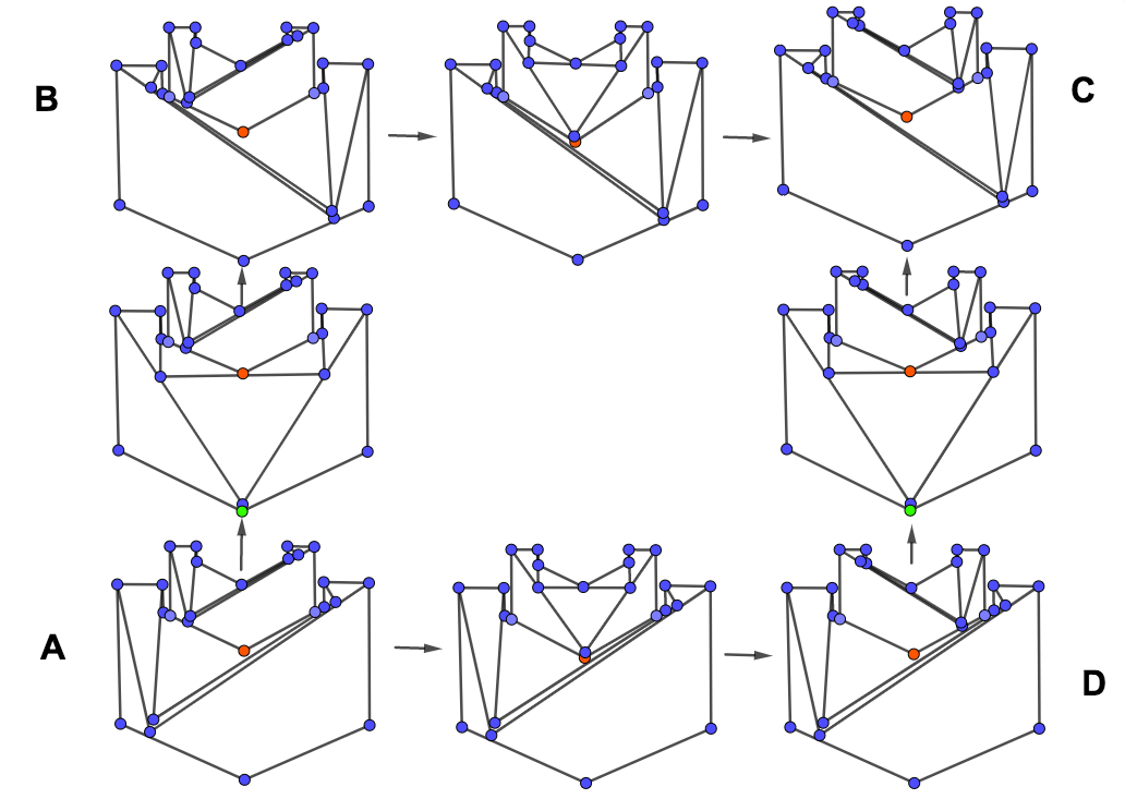
Starting with the configuration $\mathbf{A}$, we construct two paths connecting $\mathbf{A}$ and $\mathbf{C}$, shown as the paths $\mathbf{A}\to\mathbf{B}\to\mathbf{C}$ and $\mathbf{A}\to\mathbf{D}\to\mathbf{C}$. In the first path, move the vertex $G$ upward so that $\mathcal{P}_{1}^{\prime}$ is an admissible perturbation of $\mathcal{P}_{1}$. Then we can slide the vertex $P_{1}$ from the left to right to reach the configuration $\mathbf{B}$. Then move $G$ down so that $\mathcal{P}_{2}^{\prime}$ is an admissible perturbation of $\mathcal{P}_{2}$. Slide the vertex $P_{2}$ from the left to right to the configuration $\mathbf{C}$. In the second path, the order is reversed: first move $G$ down to slide $P_{2}$ from the left to right to the configuration $\mathbf{D}$, then move $G$ up to slide $P_{1}$ to the configuration $\mathbf{C}$.

We claim that the two paths above are not homotopic. Equivalently, the loop $\mathbf{A}\to\mathbf{B}\to\mathbf{C}\to\mathbf{D}\to\mathbf{A}$ represents a non-trivial element in $\pi_{1}(X(\Omega^{1},T^{1}))$.

It follows from two observations: if we project this loop to the $x$-coordinate of the vertex $P_{1}$ and $x$-coordinate of the vertex $P_{2}$ with suitable rescaling, the image of the loop is the cycle in the plane in Figure 8.

The point $(t_{0},t_{0})$ lies inside the cycle, but is not in the image of the projection of $X(\Omega^{1},T^{1})$. If the $x$-coordinate of $P_{1}$ is $t_{0}$, then the vertex $G$ has to be moved upward by Lemma 4.2. Similarly, the fact that the $x$-coordinate of $P_{2}$ equals $t_{0}$ implies that $G$ has to be moved downward. This is a contradiction.

Hence this cycle is not trivial in $\textbf{proj}_{x}^{P}(X(\Omega^{1},T^{1}))$. Hence the loop $\mathbf{A}\to\mathbf{B}\to\mathbf{C}\to\mathbf{D}\to\mathbf{A}$ is not trivial in $X(\Omega^{1},T^{1})$. A rigorous proof is given in the next section.

For any $n\geq 1$, we stack $n+1$ copies of $\mathcal{P}$ together to construct the polygons $\Omega^{n}$ with triangulation $T^{n}$. Denote these copies of $\mathcal{P}$ by $\mathcal{P}_{i}$ for $i\in I=\{1,2,\cdots,n+1\}$. Let $P_{i}$ be the corresponding vertex $P$ of $\mathcal{P}$ in each $\mathcal{P}_{i}$ for $i\in I$.

Start with the first copy $\mathcal{P}_{1}=\mathcal{P}$. Given the fact $\angle A^{\prime}KA+\angle D^{\prime}GD=360^{\circ}$, we can inductively identify the vertex $K_{i+1}$ of $\mathcal{P}_{i+1}$ with the vertex $G_{i}$ of $\mathcal{P}_{i}$, and the wedge $\angle A^{\prime}_{i+1}K_{i+1}A_{i+1}$ with part of $\angle D^{\prime}_{i}G_{i}D_{i}$ by similarity transformations of the plane

to construct $\Omega^{n}$. Define $\mathcal{P}_{i}$ in $\Omega^{n}$ to be the image of $\mathcal{P}$ under the similarity transformations $g_{i}$. Note that $g_{1}$ is the identity map of $\mathbb{R}^{2}$ with $a_{1}=1$ and $b_{1}=0$. Each $\mathcal{P}_{i}$ is a subgraph of the $1$-skeleton of $T^{n}.$

Figure 9 shows the polygon $\Omega^{n}$ with three copies of $\mathcal{P}$ stacked together. Notice that there is a small gap between two consecutive copies of $\mathcal{P}$ by proper choices of similarity transformations. We will show that for any $n>0$, $X(\Omega^{n},T^{n})$ has non-trivial $n$-th homotopy group.

To prove the new result of this paper, we first establish the existence of admissible perturbations of $\mathcal{P}_{i}$ for $i\in J$, where $J$ is strict subset of $I$.

We construct geodesic triangulations on $\Omega^{n}$ by combining geodesic triangulations of each $\mathcal{P}_{i}$, or their admissible perturbations $\mathcal{P}_{i}^{\prime}$ for $i\in I$. Define a path in $X(\mathcal{P}^{\prime}_{i},T)$ by

The path $\gamma(t)$ is constructed in Lemma 4.2 with $c=(2+\sqrt{2})/(3+\sqrt{2})$. A geodesic triangulation in $X(\mathcal{P}^{\prime}_{i},T)$ can be regarded as a part of a geodesic triangulation in $X(\Omega^{n},T^{n})$, determining the positions of $P_{i}$, $L_{i}$, and $R_{i}$. Start with a geodesic triangulation in $X(\Omega^{n},T^{n})$ such that the positions of $P_{i}$, $L_{i}$, and $R_{i}$ are given by $\gamma_{i}(-c)$. The path $\gamma_{i}$ in $X(\mathcal{P}^{\prime}_{i},T)$ produces a path in $X(\Omega^{n},T^{n})$ with $\textbf{proj}_{x}^{P_{i}}(\gamma_{i}(t))=a_{i}t$ for $t\in[-c,c]$. Notice that this path only moves three vertices $P_{i}$, $L_{i}$, and $R_{i}$ in $\mathcal{P}_{i}^{\prime}$ and fixes all the other vertices.

Combining paths above, we can simultaneously move vertices $P_{i}$, $R_{i}$, and $L_{i}$ after suitable admissible perturbations. Start with a geodesic triangulation in $X(\Omega^{n},T^{n})$, whose vertices $P_{i}$, $R_{i}$, and $L_{i}$ are determined by $\gamma_{i}(-c)$. By Lemma 4.3, for any strict subset $J=\{i_{1},i_{2},\cdots,i_{m}\}$ of $I$, there exist admissible perturbations of $\mathcal{P}_{i_{k}}$ such that $X(\mathcal{P}_{i_{k}}^{\prime},T)$ is path-connected for $i_{k}\in J$. Then each $\gamma_{i_{k}}(t)$ for $i_{k}\in J$ defines a path in $X(\Omega^{n},T^{n})$, which restricts to the identity map except in $\mathcal{P}_{i_{k}}^{\prime}$.

For any $(y_{1},\cdots,y_{m})$ with $|y_{k}|\leq c$, we define $\Gamma(\pm c,\cdots,\pm c,y_{1},y_{2},\cdots,y_{m})$ to be the geodesic triangulation in $X(\Omega^{n},T^{n})$ which is determined by $\gamma_{i_{k}}(y_{k})$ for $i_{k}\in J$ and $\gamma_{i}(\pm c)$ for $i\not\in J$. This means that the positions of $P_{i_{k}}$, $L_{i_{k}}$, and $R_{i_{k}}$ are determined by paths $\gamma_{i_{k}}(y_{k})$ if $i_{k}\in J$, and all the other vertices are fixed at $\gamma_{i}(\pm c)$ for $i\not\in J$. Using the map $\Gamma$, we prove that

References

- [1] Noam Aigerman and Yaron Lipman, Orbifold tutte embeddings., ACM Trans. Graph. 34 (2015), no. 6, 190–1.
- [2] Marwan Awartani and David W Henderson, Spaces of geodesic triangulations of the sphere, Transactions of the American Mathematical Society 304 (1987), no. 2, 721–732.
- [3] RH Bing and Michael Starbird, Linear isotopies in , Transactions of the American Mathematical Society 237 (1978), 205–222.
- [4] Ethan D Bloch, Robert Connelly, and David W Henderson, The space of simplexwise linear homeomorphisms of a convex 2-disk, Topology 23 (1984), no. 2, 161–175.
- [5] Steward S Cairns, Deformations of plane rectilinear complexes, The American Mathematical Monthly 51 (1944), no. 5, 247–252.
- [6] Stewart S Cairns, Isotopic deformations of geodesic complexes on the 2-sphere and on the plane, Annals of Mathematics (1944), 207–217.
- [7] Jean Cerf, About the bloch-connelly-henderson theorem on the simplexwise linear homeomorphisms of a convex 2-disk, arXiv preprint math/1910.00240 (2019).
- [8] Robert Connelly, David W Henderson, Chung Wu Ho, and Michael Starbird, On the problems related to linear homeomorphisms, embeddings, and isotopies, Continua, decompositions, manifolds, 1983, pp. 229–239.
- [9] Éric Colin De Verdière, Michel Pocchiola, and Gert Vegter, Tutte’s barycenter method applied to isotopies, Computational Geometry 26 (2003), no. 1, 81–97.
- [10] Y Colin de Verdiere, Comment rendre géodésique une triangulation d’une surface, L?Enseignement Mathématique 37 (1991), 201–212.
- [11] Peter Duren, Harmonic mappings in the plane, vol. 156, Cambridge university press, 2004.
- [12] Michael Floater, One-to-one piecewise linear mappings over triangulations, Mathematics of Computation 72 (2003), no. 242, 685–696.
- [13] Michael S Floater, Mean value coordinates, Computer aided geometric design 20 (2003), no. 1, 19–27.
- [14] Michael S Floater and Craig Gotsman, How to morph tilings injectively, Journal of Computational and Applied Mathematics 101 (1999), no. 1-2, 117–129.
- [15] Steven Gortler, Craig Gotsman, and Dylan Thurston, Discrete one-forms on meshes and applications to 3d mesh parameterization, Computer Aided Geometric Design (2006).
- [16] Joel Hass and Peter Scott, Simplicial energy and simplicial harmonic maps, arXiv preprint arXiv:1206.2574 (2012).
- [17] Chung Wu Ho, On certain homotopy properties of some spaces of linear and piecewise linear homeomorphisms. i, Transactions of the American Mathematical Society 181 (1973), 213–233.
- [18] Michael Kapovich and John J Millson, Universality theorems for configuration spaces of planar linkages, Topology 41 (2002), no. 6, 1051–1107.
- [19] Stephen Smale, Diffeomorphisms of the 2-sphere, Proceedings of the American Mathematical Society 10 (1959), no. 4, 621–626.
- [20] Vitaly Surazhsky and Craig Gotsman, Controllable morphing of compatible planar triangulations, ACM Transactions on Graphics (TOG) 20 (2001), no. 4, 203–231.
- [21] by same author, Intrinsic morphing of compatible triangulations, International Journal of Shape Modeling 9 (2003), no. 02, 191–201.
- [22] William Thomas Tutte, How to draw a graph, Proceedings of the London Mathematical Society 3 (1963), no. 1, 743–767.