Analysis of tensor methods for stochastic models of gene regulatory networks
Abstract
The tensor-structured parametric analysis (TPA) has been recently developed for simulating and analysing stochastic behaviours of gene regulatory networks [Liao et. al., 2015]. The method employs the Fokker-Planck approximation of the chemical master equation, and uses the Quantized Tensor Train (QTT) format, as a low-parametric tensor-structured representation of classical matrices and vectors, to approximate the high-dimensional stationary probability distribution. This paper presents a detailed error analysis of all approximation steps of the TPA regarding validity and accuracy, including modelling error, artificial boundary error, discretization error, tensor rounding error, and algebraic error. The error analysis is illustrated using computational examples, including the death-birth process and a 50-dimensional isomerization reaction chain.
keywords
stochastic chemical reaction networks, tensor method, chemical Fokker-Planck equation, high-dimensional problemsmmsxxxxxxxx–x
1 Introduction
1.1 Stochastic modelling
We briefly review the two widely-used mathematical formulations of stochastic reaction networks. A well-mixed chemically reacting system of distinct molecular species inside a reactor of volume is described, at time , by its -dimensional state vector
where is the number of molecules of the -th chemical species. We assume that molecules interact through reaction channels
| (1) |
where and are the stoichiometric coefficients. The kinetic rate parameters, , characterise the speed of the corresponding chemical reactions. Let be the probability of the system being in the state in the steady state. The exact description of such probability is the stationary chemical master equation (CME) of the form
| (2) |
where denotes the CME operator, and represents the step operator that replaces the arguments of some function by , i.e., . We denote by the -th column of the stoichiometric matrix, , with . The propensity function is an interpretation of the occurrence tendency of the -th reaction. Using the mass action kinetics, the propensity functions are of the form
for , where stands for the order of the reaction . Since the elementary reactions often involve at most interactions of two molecules, it is often assumed that for all .
Seeking satisfying (2) is the problem of finding the kernel of the linear operator . It can be interpreted as finding the eigenfunction corresponding to the zero eigenvalue of . It can be shown that the CME (2) has a unique solution satisfying the natural normalization condition Solving this exactly is intractable in general, however, it is possible to truncate the positive orthant by imposing a sufficiently large maximum copy number of each chemical species based on the reachability of states [4]. Then the solution is approximately computed as the principal eigenfunction of a finite dimensional truncation of .
One of the main disadvantages of the CME (2) is its analytical intractability for reaction systems which involve higher-order reactions. Kramers [10] and Moyal [17, 6] derived a continuous approximation of the stationary CME as a linear, diffusion-convection partial differential equation as
| (3) |
where the diffusion and drift coefficients are respectively given by
| (4) |
The domain of definition, denoted as , is an open domain such that the ellipticity condition is satisfied, i.e.,
| (5) |
Eq. (3) is known as the stationary chemical Fokker-Planck equation (CFPE). It describes how likely the system will be in a certain portion of the state space, rather than a particular integer state in (2). So a major and important difference between the CME and the CFPE is that is a non-negative integer for the CME and a real number for the CFPE.
The question of boundary conditions for the CFPE (4) is delicate, because unlike the CME, which guarantees that the support of the probability density lies within the positive orthant, the CFPE can give rise to negative copy-numbers of the chemical species. We will consider to be a function defined in as a solution of (3), and satisfy the nomalisation condition . It can be shown that, for sufficiently large system volume , the stationary distribution is bounded and unique in , with vanishing values along the boundary . We refer the readers to [32] for details on this issue.
Analytical solutions of CFPE remain elusive for many complex biological systems, and numerical simulation techniques are essential in practical applications.
1.2 Tensor formalism
A fundamental difficulty of the traditional approaches to solve the CME (2) and the CFPE (3) is the so-called curse of dimensionality [27]. It refers a universal feature of classic matrix-vector-based data format that the memory requirements and computational complexity of basic arithmetic operations grow exponentially in the number of dimensions, . As a consequence, both equations (2) and (3) have been historically simulated using the kinetic Monte Carlo methods, such as the Gillespie stochastic simulation algorithm (SSA) [5] and its equivalent formulations [22, 47]. These approaches generate statistically correct trajectories, and sample probability distributions. A disadvantage is that they require many realizations to sample in the very low probability regions, or rare events.
Tensor representation has recently been developed to address the “curse of dimensionality” [38]. Tensors are multidimensional arrays of real numbers, upon which algebraic operations generalizing matrix-vector-based operations can be performed. Through generalizing the singular value decomposition (SVD) for matrices to tensors, one could obtains various low-parametric representations of tensors, such as canonical polyadic (CP) representation [7], Tucker representation [21], tensor train (TT) representation [13], and hierarchical Tucker representation [20]. Recently, the time-dependent version of the CME (2) has been re-formualted into tensor formats, and solved directly using the time-stepping procedures under the tensor framework [39, 34, 42].
In [33], the authors introduced the tensor parametric analysis (TPA) and solved the high-dimensional stationary CFPE (3) using the recently proposed Quantized Tensor Train (QTT) format. Table 1 demonstrates the simulation steps of the TPA method. Each step introduces a different type of approximation, and contributes an additional error to the resulting approximate solution of the stationary CME (2). Therefore, in this paper, we undertake a detailed analysis of the validity of all these approximation steps, and study the convergence of different sources of error that the TPA method incurs.
(a1) The solution of the stationary CME (2), , is approximated by the solution of the stationary CFPE (3), .
(a2) The CFPE is truncated into a bounded domain and approximated by given by a Dirichlet eigenvalue problem .
(a3) The Dirichlet eigenvalue problem in the bounded domain is discretised by a finite difference scheme and is approximated by a discrete solution .
(a4) The discrete problem is solved using the QTT tensor format and the tensor rank of the discrete operator is is truncated. Consequently, the discrete solution is approximated by a tensor format solution .
(a5) The truncated tensor problem is solved by a tensor-structured iterative method. After iterations, the algorithm generates a QTT tensor as an approximation of .
1.3 Error identification
Starting from step (a1) to (a5), the error in each step is identified. Detailed mathematical formulations and studies of all these steps are presented separately in Sections 2–6, and numerical verifications are given in Section 7. We summarise our results below.
Modelling error
In step (a1), the CME (2) is approximated by the CFPE (3). The approximation is obtained by a perfunctory second-order truncation of the Taylor expansion of the CME (see Section 2.1) [6]. A few studies have suggested the CFPE’s validity in the thermodynamic limit, where the system volume approaches to infinity. Kurtz [41] proves that the difference between the jump and continuous Markov processes is of order . Grima et al. [28] used system-size expansion to show the CFPE predictions of the mean and the variance are accurate to order . Here, the tensor methods seek to simulate the whole probability distribution, rather than the summary statistics, the error between the CME and the CFPE distributions are of main interest. In Section 2, we apply the system-size expansion techniques in [28] to estimate the -norm between and . In Theorem 2, we show that the difference is of order for general reaction networks. We also provide a tighter bound as in Theorem 4 for systems satisfying the detailed balanced condition.
Artificial boundary error
In step (a2), the TPA solves the Dirichlet eigenvalue problem on a bounded domain in which the vast majority of the probability density sits, and then uses the resulting principal eigenfunction in to approximate the exact stationary distribution in . We show in Theorem 5 that converges toward as . We also use a numerical experiment (Fig. 1(b)) in Section 7.1 to show the convergence rate of the error between and within agrees well with the maximum gradient at boundaries, i.e., .
Discretization error
In step (a3), the TPA uses the finite difference approximations of the (elliptic) Dirichlet eigenvalue problem. Although many authors [19, 18, 11] have studied the convergence of difference schemes for selfadjoint eigenvalue problems, non-selfadjoint problems in higher dimensions are less studied [2], because it is generally not possible to build a monotone difference scheme using a narrow stencil [46]. Recently, a monotone and conservative difference scheme for elliptic operators with mixed derivatives has been proposed [1, 16, 25]. The scheme is useful to discretise the CFPEs in lower dimensions, but it is difficult to formulate in tensor formats, and thus may hardly be applied to higher dimensions. In Section 4.1, we tailor the difference scheme such that it is capable to address the high-dimensional Fokker-Planck Dirichlet eigenvalue problem, and enjoys precise tensor decomposition (see Section 5.1). The difference scheme generates an irreducible -matrix as the assembled matrix (Lemma 6), under appropriate conditions on the stoichiometric coefficients (Remark 7). We prove in Theorem 8 that it gives a second order accurate approximation of both the principal eigenvalue and eigenfunction, which is also validated numerically (Fig. 1(c)).
Tensor rounding error
Step (a4) of the TPA introduces the tensor representations to the traditional finite difference discretization. Thanks to the new compact difference scheme (in step (a3)), we show in Section 5.1 that the assembled matrix of the CFPE operator admits exact canonical tensor representation as a sum of canonical tensor products (CP format [7]), with tensor ranks bounded by (Proposition 9). In Section 5.2, the CFPE operator in CP format is then restructured into TT format under the same rank bound (Lemma 10). In Section 5.3, the TT matrix operator is further suppressed by the QTT representation, and Theorem 11 gives the storage requirement for the CFPE operator in the QTT format to be of order , where is the number of grid nodes in each dimension. Moreover, once the assembled matrix is already represented in the QTT format, such storage estimate could be further reduced by an algorithm that truncates the tensor separation rank [15]. The truncation introduces perturbations to the entries of the original QTT matrix, and Theorem 12 links the perturbed tensor eigenvalue problem to the traditional matrix perturbation theory [3], and present a linear convergence of the tensor rounding error. In the numerical experiment (Fig. 1(d) in Section 7.1), we find the effect of the tensor rounding could go beyond the linear region.
Algebraic error
In step (a5), the TPA uses a tensor-structured inverse power method to search for a low-rank approximation of the principal eigenfunction in QTT format (see Algorithm 18). In order to legitimise this approach, we derive conditions (assumptions) in Section 6.1, such that there exist desirable low-rank approximations [8]. We show in Proposition 16 that the existence of low-rank QTT approximation of a distribution is determined by the fact that whether the distribution could be expressed by a sum of a minimum number of Gaussian functions. These Gaussian functions should be away from the boundaries, and the boundary effects are not significant (Lemmas 13 and 14). Under such conditions, we show there exists a QTT -approximation with ranks bounded by (see Remark 17). It means that one saves the storage of order by allowing a tensor approximation error . The existence also legitimises our use of the truncated inverse iterations to search for low-rank QTT -approximations. Further in Theorem 20, we show that, if one allows -approximations to all intermediate solutions of the inverse iterations, the whole procedure still converges to the exact principal eigenfunction, with the algebraic error of order (Remark 21). The estimate on the algebraic error is confirmed in the numerical experiment in Fig. 2 of Section 7.1.
2 Modelling error
We will now investigate the convergence of the Fokker-Planck approximation (3) of the master equation (2) in the limit of large volumes , the so-called thermodynamic limit. Specifically, our main interest here is to derive the leading order error in the difference of the distribution,
where and are the solutions of (2) and (3), respectively. We will derive the leading order error by comparing the system size expansions (SSEs) of the CME and the CFPE.
2.1 System-size expansion of the CME and the CFPE
In this section, following the original development by Van Kampen [23], we carry out the system size expansion of the time-dependent CME,
| (6) |
where represents the time-dependent CME distribution. Later, we will extend the SSE to expand the CFPE. The starting point of the SSE is performing the change of variables, or ansatz,
| (7) |
where the instantaneous molecular population is decomposed into a deterministic part and a fluctuation part . The distribution of the fluctuations is denoted by , and in the large volume limit, the change of variable (7) implies .
The derivation of the CME in the new variables is performed by expanding the step operators and the propensity functions. Taylor expanding the step operator yields
where for and . For the propensity functions, the Taylor expansion series can be written as
| (8) |
and further the term can be expanded as
| (9) |
and the coefficients are given by
| (10) |
where denotes the Stirling number of the first kind. Then, substituting (9) into (8) yields the series expansion of the propensities, written as
where for and .
Substituting the expansions (8) and (9) into the CME (6), and rearranging the results in the inverse power of , we have the CME in the new variables as
| (11) |
where, for notational simplicity, we define the operator on order in the form
In (11), the leading order terms cancel out given the condition that satisfies the deterministic reaction rate equation.
Analogously, we can apply the same expansion procedure to the time-dependent CFPE, written as
| (12) |
Let be the transformed version of the CFPE distribution by the change of variables (7). Then, it can be shown that satisfies the following SSE expanded equation of the form
| (13) |
where
2.2 Perturbative analysis of the modelling error
Next, we focus on the stationary case and assume that trajectories of the deterministic reaction rate equation converge to a stable fixed point, . We write the stationary quantities by dropping their time dependence, i.e., and . Next, we perform the perturbative analysis of the CME (11) and the CFPE (13) in new variables to derive the leading order error between and .
We consider expressing distribution in terms of a perturbation series in inverse powers of square root of system volume as
| (14) |
Substituting (14) into (11) and equating the terms of order yields the equation for the expanded coefficients as
| (15) |
with normalisation conditions and , . Analogously, we write the series expansion of the CFPE distribution as , and the equations for the expanded coefficients are given by
| (16) |
satisfying normalisation conditions and , . Both equations (15) and (16) has the similar form where the coefficient are determined by the coefficients and operators on the lower orders, thus the leading order error between and can be found by comparing operators on the increasing orders.
Lemma 1.
For sufficiently large volume size , we have
| (17) |
where is a constant independent of .
Proof.
Given the expansion series as in (14), we can express the error between and in the same form as
| (18) |
where and satisfy (15) and (16), respectively. For , the right-hand sides of both equations equal to zero and thus we have . For , the difference between the operators follows , which is non-zero in general, and thus the coefficients do no equal, i.e., . Hence, the higher order error can be bounded by , which guarantees the convergence in (17). ∎
Given the difference between the distributions of the fluctuations in (17) of Lemma 1, one can back up the error between the CFPE distribution and the CME distribution , using the scaling relationship in (7).
Theorem 2.
For sufficiently large volume size , we have
| (19) |
where is the number of chemical species and is a constant independent of .
2.3 Systems with detailed balanced condition
The error convergence (19) of Theorem 2 applies to the general types of reaction networks (1) that fulfil the assumption that the trajectories of the deterministic reaction rate equation converge to a single fixed point. Next, we consider a type of networks obeying the detailed balanced condition.
Definition 3.
A chemical reaction network is called reversible, if for every reaction of the form (1) with a positive reaction rate , there exists a backward reaction with a positive reaction rate . Further, a reversible reaction network is detailed balanced, if for each pair of reversible reactions, we have
| (20) |
where are the deterministic rate functions defined in (10) with the plus and minus signs referring to the forward and backward reactions, respectively.
Applying the condition (20) of Definition 3 to the equations (15) and (16) of the expansion coefficients, one can derive a higher order convergence between the CME and CFPE distributions.
Theorem 4.
Assuming the detailed balanced condition in Definition 3 is satisfied, then for sufficiently large volume , we have
| (21) |
where is a constant independent of .
Proof.
We have shown in Lemma 1 that and agree on order , and now we prove they also agree on order given the detailed balanced condition. The difference between the operators and is given by
where the last formula is derived from the detailed balanced assumption that the reactions come in pairs and the fact that the stoichiometric coefficients for the backward reaction is the same as the forward one but with the opposite sign. Substituting the condition (20) into the above formula yields , and from (18), we can derive
which is an analogy of Lemma 1. Then as before, reversing back the change of variables in (7) gives the convergence in (21). ∎
3 Artificial boundary error
For the purpose of computation, the stationary CFPE (3) is only considered in a bounded domain, , and the stationary solution is approximated by the positive principal eigenfunction,
| (22) |
where denotes the truncated CFPE operator within , and represents the principal eigenvalue. We consider the homogeneous Dirichlet boundary condition as the artificial boundary condition on , i.e.,
Since is a subset of , the ellipticity condition is satisfied in . In fact, it can be shown that the sufficient conditions for fulfilling the ellipticity condition (5) are (a) for all and all and (b) there is (out of ) linearly independent rows of the stochiometric matrix .
Theorem 5.
If the stationary CFPE (3) admits an bounded solution in , which is unique up to a constant multiplication. Then, for , we have
If further both and are normalised so that for a given , we have the convergence in as .
Proof.
Assuming the existence and uniqueness of solution in (3) implies a zero (generalised) principal eigenvalue of in . Using Proposition 2.3(iv) in [12], we obtain a negative principal eigenvalue of operator in , and its convergence as . The convergence of the eigenfunctions is given in the proof of Theorem 1.4 in [12]. ∎
4 Discretization error
In this section we present and analyse a monotone difference scheme for the (generalized) Fokker-Planck eigenvalue problem (22). We follow the traditional matrix-vector-based routine in the current section where the nodal points are enumerated by one index and the corresponding discretised functions are stacked into a “long” vector, but we will consider storage compression by tensor representation in section 5.
4.1 Difference scheme
In an -dimensional hypercube , , we consider the uniform grid :
with constant grid step . The set of boundary grid points is . Let us consider the following notation conventions of difference operator at grid :
| (23) | ||||
where and represent the partial sums of the positive and negative terms in (4), respectively, i.e.,
| (24) |
Then, the finite difference approximation of (22) of second order reads
| (25) |
where here denotes a huge multi-dimensional matrix, and is the associate principal eigenpair of . The stencil of difference scheme (23) is compact, that uses only surrounding nodes for its discretization in dimensions. For investigation of a priori error estimate of the solution , the following result has been proved in Theorem 3.7 of [32], and we presented in the following lemma.
Lemma 6.
Let us suppose that, for sufficiently small grid size , , the following conditions are satisfied:
| (26) |
then the stiffness matrix in (25) is an irreducible -matrix, and the principal eigenpair of has the following properties: (i) is real and algebraically (and geometrically) simple; (ii) and for every eigenvalue ; and (iii) for all .
Remark 7.
Lemma 6 suggests that the difference scheme (25) satisfies the discrete maximum principle, and is stable and convergent. Note that, if stoichiometric coefficients of (1) satisfy the following inequality
| (27) |
then one can choose which guarantees that condition (26) is satisfied. To fully satisfy the condition of Lemma 6, we further require small enough such that the drift terms in (25) are small enough to keep the positivity of the off-diagonal entries in .
4.2 Convergence of discretization error
Let be the eigenvalues of , considered as approximations to the first eigenvalues of the differential operator in (22). For a positive integer we define to be the eigenvector corresponding to , normalised so that . We will show the convergence rate of and to the continuous problem in (22) as the grid size , , in the following theorem.
Theorem 8.
Let , be principal eigenpairs of with . Let be an eigenfunction of associated with , and let be the vector obtained from by grid point evaluation in . Assume normalised so that . Define for , that satisfies the conditions of Lemma 6 then as , we have
| (28) |
where , are positive constants.
Proof.
Because the difference scheme (25) is properly centered and we assume sufficient smoothness of , we have
| (29) |
where is the truncation error of the difference scheme. One can show, by using Taylor expansion in space [1], that
| (30) |
where is a constant depending on . Now we write as a linear combination of the eigenvectors of , i.e.,
| (31) |
Substituting into (29) gives
| (32) |
Let be the normalised principal left eigenvector of corresponding to , then multiply to both sides of the equation (32) and use the relation in (30), we have
| (33) |
where is a constant depending only on , , , and . We may assume , and divide both sides of the inequality by . This gives the convergence rate of the principal eigenvalue in (28).
Now we derive the convergence of the eigenvector towards . Let be a matrix formed by the columns of the right eigenvectors of , then the matrix form of (31) reads , where denotes a column vector with entries . Similarly, the matrix form of (32) is given by
| (34) |
where is a diagonal matrix with , , as the diagonal entries. From Lemma 6, is a simple eigenvalue of , and is linearly independent with , . Thus we can define a transformation that makes , , orthogonal to . We define matrix as
where denotes the inner product of vectors and . Let , then the first column of is orthogonal to all other columns. Then, multiplying to both sides of (34) gives
| (35) |
From the definition of , the structure of is of the form
where is an submatrix of with the first column vector removed. It can also be verified that
where refers to a vector formed by the first row of matrix except the first element. Further, since is diagonal matrix, we can reduce (35) to
where is a submatrix of with the first row and the first column removed, and is a sub-vector of with entries . Then, we have
| (36) |
with constant , where we have assumed that eigenvectors have bounded entries, i.e., . In above inequality, we notice that . Since we have proved the convergence of the eigenvalue towards , for sufficiently small , there exists a positive constant , such that
We can further bound in (36) by
where is a constant. We may need to assume the eigenvectors, , , are bounded. It then follows that
where is a constant. The above inequality gives the convergence of principal eigenvector in (28). ∎
5 Tensor-structured approximation
In this section we discuss the tensor representation of the difference scheme (25), and the associate error caused by the separation rank truncations.
5.1 Canonical tensor products applied to Fokker-Planck problem
The tensor product (Kronecker product, direct product) of two matrices and , denoted by , can be written as a matrix in block partition form
| (37) |
A detailed account of properties of tensor product is given in [24]. Some of the elementary properties are:
For brevity, we do not indicate explicitly the sizes of the matrices involved; we assume throughout that the sizes of matrices and vectors are compatible with the indicated operations. We will refer the tensor product of matrices as rank-1 tensor matrix, and sum of rank-1 tensor matrices as rank- matrix, both denoted in bold font capitals.
For compact finite difference scheme (23), it is readily verified that the upwind difference and the downwind difference are, respectively, of the form
| (38) |
for , where denotes identity matrix of appropriate sizes. The upwind difference matrix has entries and distributed along its super-diagonal and diagonal, and the downwind difference matrix has them alone its diagonal and sub-diagonal. It follows that the tensor representation of the difference operator in (23) reads
| (39) |
for , where and are the tensor matrix representations of the positive and negative summation of diffusion coefficients, and , in (24) of the form
and is the tensor representation of the drift coefficients, , in (4) of the form
where is a rank-1 representation of propensities, , by
| (40) |
for , and
for , and , where was defined in Section 1. Then the tensor analogy of finite difference discretization of Fokker-Planck equation in (25) reads
| (41) |
where is an exact permuted reformulation of in (25) as a sum of rank-1 tensor matrices, and stands for the canonical tensor representation of the “long” vector . The separation rank bound of is given as follows..
Proposition 9.
The rank bound can be directly derived from the explicit structure of in (41). It scales quadratically in and linearly in , that indicates the storage requirement of the assembled canonical tensor matrix scales as , for , .
5.2 Tensor train representation
The tensor train (TT) representation of the canonical matrix can be described as
| (42) |
where the core tensors are defined as for , for , and for . The generalised mode- product of two TT matrices, and , yields TT matrix with entries . The sizes of bridging dimensions are called the ranks of the TT matrix. The canonical representation (41) can be directly converted to the tensor train representation (42) and the ranks of the resulting TT matrix are given in the following lemma, where stands for the Frobenius norm.
Lemma 10 (Corollary 2.3 in [13]).
If a tensor matrix admits a canonical representation with rank and accuracy , then there exists a TT representation with TT-ranks and accuracy .
5.3 Quantized tensor train representation
We have discussed using the tensor representation to break the curse of dimensionality in physical dimensions of the state space . Now, each of the physical dimension is further quantized into several virtual dimensions, and consequently, each of the core tensors in (42) is further decomposed as the product of quantized core tensors with smaller mode size.
Consider tensor in (42) with core tensors and , , , the mode index can be mapped to binary representation with the quantized indices , , i.e., . Then the quantized decomposition of core tensors , is given by
| (43) |
where for , for , and for . In case where or , the decompositions of the core tensors are identical to (43), except that for , and for .
Substitute the quantized core tensors of the form (43) into the TT representation (42), the resulting decomposition is the so-called quantized tensor train (QTT) [43]. An upper bound on the ranks of QTT representation for the Fokker-Planck operator, , is given in the following theorem.
Theorem 11.
Proof.
A detailed proof of the above theorem is given in section 3.2.2.5 in [32]. ∎
A slightly crude upper rank bound can be derived from Theorem 11. Let , we have
which suggests the QTT-rank is of order . Subsequently, the QTT representation of Fokker-Planck operator has complexity estimate to be , logarithmic scaling in volume size.
5.4 Tensor rounding error
Once the assembled tensor matrix is already in the QTT representation as in (43), we want to have an approximation, , with the “optimal” ranks such that
where is the required accuracy level. Here, denotes any vector norm for vector , and denotes the corresponding matrix norm. Let , , be the QTT-ranks of , and let , under certain assumptions [44], the suboptimal rank bound scales with as
Such a procedure is usually called rounding (truncation or recompression), and as a consequence, the truncated ranks may be significant lower than the rank bound given in Theorem 11.
The approximated elliptic eigenvalue problem after tensor rounding reads
| (45) |
where stands for the principal eigenpair of , and represents the perturbation caused by tensor rounding. It is of interest here to obtain bounds for the differences and . Such error bounds can be analogically obtained as the perturbation bounds for the principal eigenvalues and eigenvectors of corresponding matrices [3]. We state it as following theorem.
6 Algorithm
In this section, we discuss solutions of the tensorised eigenvalue problem. First of all, in section 6.1, we show there exist low-rank tensor approximations to the principal eigenfunctions under certain assumptions. Then, in section 6.2, we present an inverse scheme in tensor formats that aims to search for such low-rank approximations. Finally in section 6.3, we study the algebraic error of the proposed algorithm.
6.1 Existence
As an analogy of (42) with (43), the QTT approximation of with , , reads
| (47) |
where stands for the mode- product of two tensors, and the quantized core tensors are of the form
| (48) |
where for , for , and for . In case where or , the decompositions of the core tensors are identical to (48), except that for , and for . Before presenting any algorithm to seek such an approximation , we are interested in understanding whether there exists a low-rank -approximation, i.e., satisfying .
6.1.1 Gaussian distributions
To answer such a question in a general scenario, we start with the cases where the solution is a Gaussian distribution. In single-dimensional cases, the rank bounds are subject to the following lemma.
Lemma 13 (Lemma 2.4 [35]).
Suppose uniform grid points , , , are given on an interval and the vector is defined by its elements . Suppose in addition that . Then for all sufficiently small there exists the QTT approximation with ranks bounded as
and the accuracy
where is a constant does not depend on , , , or .
Since the multidimensional Gaussian function is a product of one-dimensional counterparts, its canonical separation ranks are equal to 1. By the triangular inequality, an error bound of the QTT approximation in dimensions can be derived. Thus, we extend Lemma 13 to the multidimensional cases in the following lemma.
Lemma 14.
Consider an -dimensional hypercube with discretised by uniform grid nodes , where , , , . Let tensor be its elements
| (49) |
Suppose in addition that . Then for sufficiently small , there exists the QTT approximation with ranks bounded as for , and
| (50) |
and the accuracy
| (51) |
where and is a constant does not depend on , , , , or .
For fixed ’s, a more concentrated Gaussian distribution, with a larger ratio of over , would give rise to smaller separation ranks in (50) and smaller approximation error in (51). On the other hand, this could also be achieved by increasing ’s while fixing ’s and ’s.
Remark 15.
Tolerance implicitly impose restrictions on the choice of and . By requiring , we have , such that and . Thus, an estimate for approximation error w.r.t the tensor ranks could be .
6.1.2 Non-Gaussian distributions
In the following, we generalize the QTT approximation of the Gaussian solutions to the cases of more general classes of -dimensional distributions. Let us consider the class of in (47) equivalent to certain analytical functions by grid point evaluation. We assume that allows the efficient approximation in the set of Gaussian distributions on . Then we prove the following error bound for the QTT approximation.
Proposition 16.
Let with , . Suppose that for a given continuous function , and given , there is an approximation by Gaussian sums such that
| (52) |
where is the -dimensional Gaussian function defined by . In addition, we assume that . Then, consider an -dimensional tensor defined by its entries , for , , where , . It allows an QTT tensor in the form of (47), with ranks bounded by and
| (53) |
for , , and the accuracy
where is a constant does not depend on , , , , , or , and is a constant does not depend on , , or .
Proof.
We define tensors by grid evaluation of the -dimensional Gaussian , for , as in (49). From Lemma 14, there exists an QTT approximation , with ranks bounded by (50) and accuracy given by (51). Hence, we define , as a QTT approximation of , by . Using the addition rules of QTT ranks [43], the bounds in (53) can be justified.
Remark 17.
Back to our question at the beginning of this section about the existence of a low-rank -approximation to the solution of (45). Remark 17 imposes a key condition that the eigenfunctions need to be well approximated by the sum of a minimum number of Gaussian functions. And the peaks of these Gaussian functions have to be significantly away from the boundary . Unfortunately, conditions on the operator are still unclear.
6.2 Higher order inverse iteration
Remark 17 ensures that one class of the eigenvector allows a low rank QTT -approximation as in Proposition 16. To approximate the eigenpair , we use a higher order analogue of the inverse iteration, combined with tensor truncations. The main building block is as follows.
Algorithm 18 (Inverse power method in tensor format).
For till convergence do
, with ;
;
end
When the linear systems are solved precisely, i.e., , Algorithm 18, beginning with an initial tensor , the series would converge to the eigenvector corresponding to the eigenvalue closest to the chosen shift . If we assume the perturbation in (45) is sufficiently small that the matrix corresponding to remains -matrix, then from Lemma 6, any non-negative would lead to the correct convergence direction towards .
However, there are two main reasons that the residue tensor needs to be considered. First, we use the Alternating minimal energy method (AMEN) [36, 37] to conduct inner iterations to solve the linear system in QTT format in Algorithm 18. A highly accurate solution in each inverse iteration requests more computational time, and it is usually not necessary (as we will prove later). Second, tensor rounding procedure needs to be performed after each inverse iteration to avoid uncontrollable growth of the tensor separation rank [13, 31], which also adds to the residual. Therefore, it is of interest to analyse the effect of the residues on the final convergence.
6.3 Algebraic error
The error analysis of Algorithm 18 is analogous to the analysis for the inexact inverse power method [9]. Let for be a complete set of eigentriples of satisfying . It follows that
where is the Kronecker symbol. We assume that the intermediate solution after inverse iterations can be expanded as a linear combination of right eigenvectors:
| (55) |
Now we define a measure of the approximation of to for as
The convergence of is concluded by the corresponding matrix analysis, see Lemma 2 and 3 in [9], and for Algorithm 18, we state the tensor version as below.
Lemma 19.
Let , and . Let columns of tensor matrices and contain all left and right eigenvectors of , respectively. Then,
| (56) |
where .
Then we have the convergence of the algebraic error in the following theorem.
Theorem 20.
Proof.
7 Numerical illustrations
We run all our numerical experiments in Matlab solely on a MacBook Pro laptop (OS X 10.9.5) with a 2 GHz Intel Core i7 processor and 8 GB of physical memory. Our source codes made extensive use of the Tensor Train toolbox [13], and is part of the Stochastic Bifurcation Analyzer toolbox freely available at http://people.maths.ox.ac.uk/liao/stobifan/index.html [33].
7.1 1-D birth-death process
As a first application of our theory, we will estimate all sources of errors discussed in sections 2-6 for the birth-death process. This is the simplest case of a molecular reaction mechanism. The main purpose of considering such a reaction is that both its stationary CME (2) and CFPE (3) are exactly solvable and hence it provides us with a direct test of our expressions in the error estimates. The set of reactions under study are
| (58) |
A single chemical species, denoted as , is produced by some substrates within certain container of volume at a constant rate , and de-gradates with rate constant .
The CME (2) for the birth-death reactions (58) reads
| (59) |
for , where the propensities functions are
The stationary solution of (59) is the Poisson distribution
| (60) |
The corresponding Fokker-Planck approximation (3) of the CME (59) can be written as
| (61) |
for . Integrating over and using the boundary conditions as , we obtain
| (62) |
where the normalisation constant is chosen such that , i.e.
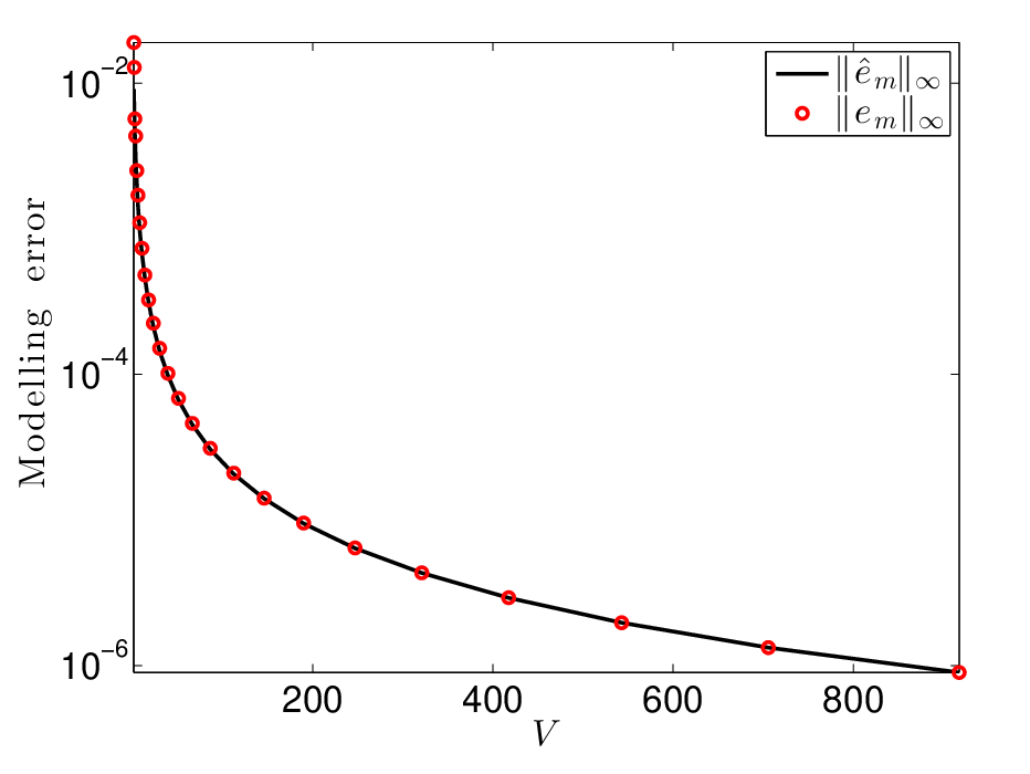
With explicit formulas (60) and (62), we evaluate the exact modelling error , and plot the error measured in -norm in Fig. 1(a) against increasing values of system volume . As comparison, we use the black curve to refer to our estimate in (21) of Theorem 4. By fitting the constant coefficients in (21) to the exact errors , we obtain a good agreement between the exact errors and the estimated ones.
Next, we consider approximating the CFPE (61) within a bounded domain . As discussed in section 3, the stationary solution in (62) is approximated by the positive principal eigenfunction , satisfying
| (63) |
where is the principal eigenvalue. In Fig. 1(b), we show the domain dependence of and . Here, we fix the center of at the mean value , and vary the domain size . In accordance with our convergence statement in Theorem 5, the numerical experiment also shows that and as increases. We also plot the changes of with respect to as the solid cure in Fig. 1(b). Such quantity represents the maximum gradient of the solution at the boundaries. We can observe that the decay rate of is similar to , indicating that both these quantities can be potentially used as error indicators for the artificial boundary error. Unfortunately, we are not able to provide theoretical proof for such argument at the moment.
(a)
 (b)
(b)

(c)
 (d)
(d)

Fig. 1(c) illustrates the grid-size dependence of the discretisation error in numerical solution of (63) using the difference scheme (25) in section 4. The discrete principal eigenfunction is computed using Matlab eigs function. The exact discretization error, , is then approximately computed by by choosing such that is sufficiently small. We could observe that the convergence of the discretization error (red circles) agrees well with our error estimate (dashed curve) derived in (8) of Theorem 28.
Following sections 5.1, 5.2 and 5.3, we now establish the QTT representation (43) of the difference scheme (25) for the eigenvalue problem (63), and test how the tensor rounding procedure of the assembled tensor matrix would cause deflection in the principal eigenpair towards . Since the error in the rounding of the tensor matrix is of the main concern, for different tolerances in tensor rounding, we always first assemble the operator in QTT format, apply TT-rounding algorithm [13] with the prescribed tolerance to truncate to form , unfold tensor matrix into the standard matrix , and then use the Matlab eigs function to compute the principal eigenpair . Here, is the equivalent vector form of the tensor . In this way, we could exactly measure the error caused by tensor rounding of the QTT matrix . In Fig. 1(d), we could see the trend that the error in -norm increases for larger tolerance values. But we could also observe that, for ranges of tolerance values, the tensor rounding error , together with , remains at a constant level. This is not predicted by our Theorem 12. The reason is that the tensor rounding algorithm is SVD-based [13], meaning that the rank truncation is based on the magnitude of the singular values rather than certain matrix norm. Therefore, it is possible that different tolerance values in tensor rounding procedure would generate the same result, especially when there exist large spectrum gaps. Also, as predicted by Theorem 11, the maximum QTT rank (43) of is 24 (see Fig. 1(d)). But even for very small tolerance values, the maximum rank of is reduced to 4, by only causing an error of order in the approximated principal eigenvector.
Next, instead of using the Matlab eigs function, we keep all objects in QTT format and solve for using the higher order inverse iteration presented in Algorithm 18. Setting the shift value , we computed the algebraic error for each of the inverse iterations. The convergences of the algebraic error in -norm under difference stopping tolerances for the tensor linear solver – AMEN [36, 37] are shown in Fig. 2(a). We see that all simulations initially converge with similar rates, and the convergence comes to a halt after certain number of iterations. This matches our prediction in Theorem 20, that for small number of iterations , the term in (57) dominates the algebraic error , while for large , the dominance is taken over by the term in (57) caused by the inexactness of the tensor linear solver (Remark 21). In Fig. 2(b), we only consider the algebraic error after inverse iterations, and plot it against different tolerance in solving the tensor linear systems. The algebraic error agrees well with the reference line in the blue dashed curve, which is the direct result from (57) in Theorem 20 for fixed and . We could also observe the increase in the tensor rank as the tolerance value decreases (solid curve in Fig. 2(b)), and the exponential scaling matches our prediction in Remark 17.
(a)
 (b)
(b)

7.2 A 50-dimensional reversible isomerization reaction chain
In this section, the simple birth-death process (58) is extended to a 50-dimensional reaction chain, where molecules are allowed to transform themselves into different isometric forms, i.e.,
| (64) |
where , , can be interpreted as the -th isometric form of species , and , , are reaction constants. The corresponding stoichiometric matrix is given by
Let be the state vector, then the propensity functions are of the form
Consider , , be the solution of the stationary CME (2) for the isometrization reaction (64), it is a product Poisson distribution [40],
| (65) |
where , , stand for univariate Poisson functions whose mean equal to the stead state solution of a system of reaction rate equations.
In comparison, the analytical formula for the solution of the stationary CFPE (3) for the isomerization reactions (64) is not obvious. Furthermore, because of the very high dimensionality, we would not be able to identify individual sources of errors separately as we did in section 7.1. This is to say that we would only be able to compute the final tensor approximation , whose accuracy depends on the accuracies of all intermediate steps (a1)–(a1) in the TPA (Table 1). Whereas there will be no intermediate solutions available to guide us to choose appropriate parameters in each step. To address this issue, we notice that the isomerization reaction chain (64) could be viewed as an extension of the birth death process (58), and thus our error analysis in section 7.1 could potentially hint the choice of parameters for simulating the extended reaction chain (64).
Let us start with a target that we wish the final tensor solution to be accurate to order in approximating the exact Poisson distribution (65). This means that we should pick simulation parameters such that all sources of errors are kept below . We choose the system volume to be consistent with the simulations of the death-birth process (58). From Fig. 1(a), the modelling error at would be far below . The computational domain is chosen as , and accordingly to Fig. 1(b), the domain size keeps the artificial boundary error below . We choose the equidistant grid size for all 50 dimensions, to keep the discretization error below as suggested by Fig. 1(c). We choose the tolerance of tensor rounding procedure to be such that the tensor rounding error in Fig. 1(d) is not significant. The tolerance for the tensor linear solver, AMEN, in the inverse iterations is chosen to be to keep the algebraic error in Fig. 1(d) below .
(a)
 (b)
(b)

(c)
 (d)
(d)

The simulation results and performances of the TPA are demonstrated in Fig. 3. The computed tensor data agrees well with the exact Poisson distribution (see Fig. 3(a)), and the accuracy meets the pre-set target in all 50 dimensions (see Fig. 3(b)). The error convergence in Fig. 3(c) matches the prediction of Theorem 20 that the error first decreases monotonically and then the convergence comes to a halt due to the inexactness in solving the tensor linear systems. But we also observe the maximum QTT rank increases dramatically in the initial inverse iterations. Larger tensor ranks give rise to quadratic complexity of basic arithmetic, and as a consequence, the first few iterations with large QTT ranks cost almost half of the computational time, while their effect in error convergence is not obvious at all (see Fig. 3(d)). This refers to a major problem in the low-rank tensor computations that, even the final solution admits low-rank approximations, the growth in the ranks of the intermediate solutions might still kills the simulation. This still remains as an open problem in this area.
Our 50-dimensional solution in QTT format has storage requirement to be , whereas this number would be if stored in a standard vector. This demonstrate the effectiveness of the tensor approach for analysing high-dimensional stochastic models of GRNs. It is also worth pointing out that the total computational time is as long as seconds using a personal laptop. Such heavy simulation highlights the crucial role of the error analysis as we have presented in the current paper, because such understanding not only has informed us about the accuracy of the method, but has also guided us with feasible choices of simulations parameters such that unnecessary repetitions could be avoided.
8 Discussion
In this paper we have presented a detailed mathematical and numerical study of the difference sources of errors in the recently proposed tensor approach [33] for simulating high-dimensional stochastic models of GRNs. The five sources of errors include: modelling error due to approximate the CME by a Fokker-Planck-type diffusion process; artificial boundary error due to the truncation of the infinite domain of definition into a computable bounded domain; discretization error in the finite difference approximations; tensor round error due to the tensor rounding procedure; and algebraic error caused by the tensor-structured inverse power method.
These errors are like the stepping stones that bridge the gap between what we get and what we expect. We emphasise in this work that the total error of the TPA, as well as many other simulation methods in the literature, never solely relies on any particular source of errors, but is orchestrated by all of them. On one hand, it warns us with the complication in the choice of simulation parameters to reduce the overall errors. On the other hand, it hints the flexibility to make computational trade-offs through controlling individual sources of errors, especially in high-dimensional computations. As we posed in the birth-death example of section 7.1, if the system volume has induced modelling error of order , it is rarely necessary to pick a small grid size or choose a small tolerance for the tensor linear solver , because it would not reduce the overall error that has already been significantly contributed by the modelling error (see Figs. 1 and 2). It is therefore reasonable to relax the restrictions on and , and the computational efficiency could be improved.
Notwithstanding that the presented analysis has been mainly tailored for the TPA, many results may be useful in a wider range of methods and applications. The modelling error estimate in Theorem 4 could be applied to analyse other stochastic simulation methods based on the Fokker-Planck formulations [6, 26, 30, 29]. The monotone difference scheme described in section 4.1 introduces the idea of applying different stencils to the positive and negative summands of the diffusion coefficients, while the existing schemes mainly separate the positive and negative parts [1]. For many elliptic and parabolic problems, the coefficients may be splitted into the summands that admit a separable form, then using our modified difference scheme, these problems can be directly equipped with tensor representations and solved in higher dimensions. Finally, our study on the algebraic error could be applied to legitimise and analyse the use of inverse power method with tensor rank truncations in many other high-dimensional eigenvalue problems [8, 45].
Acknowledgment
The author would like to thank Professor Radek Erban and Dr Tomáš Vejchodský for all of their careful, constructive and insightful comments that greatly contributed to improving the final version of the paper. The research leading to these results has received funding from the European Research Council under the European Community’s Seventh Framework Programme (FP7/2007–2013)/ERC grant agreement no. 239870.
References
- [1] A. A. Samarskii, P. P. Matus, V. I. Mazhukin, and I. E. Mozolevski, Monotone difference schemes for equations with mixed derivatives, Comput. Math. Appl., 44 (2002), pp. 501–510.
- [2] A. Carasso, Finite-difference methods and the eigenvalue problem for nonselfadjoint Sturm-Liouville operators, Math. Comp., 23 (1969), pp. 717–729.
- [3] A. S. Deif, Rigorous perturbation bounds for eigenvalues and eigenvectors of a matrix, J. Comput. Appl. Math., 57 (1995), pp. 403–412.
- [4] B. Munsky, and M. Khammash, The finite state projection algorithm for the solution of the chemical master equation, J. Chem. Phys., 124 (2006), pp. 044104.
- [5] D. T. Gillespie, Exact Stochastic Simulation of Coupled Chemical Reactions, J. Chem. Phys., 81 (1977), pp. 2340–-2361.
- [6] D. T. Gillespie, The chemical Langevin equation, J. Chem. Phys., 113 (2000), pp 297–306.
- [7] F. L. Hitchcock, The expression of a tensor or a polyadic as a sum of products, J. Math. Phys., 6 (1927), pp. 164–189.
- [8] G. Beylkin, and M. J. Mohlenkamp, Numerical operator calculus in higher dimensions, Proc. Natl. Acad. Sci. USA, 99 (2002), pp. 10246–10251.
- [9] G. Golub and Q. Ye, Inexact inverse iteration for generalized eigenvalue problems, BIT Numerical Mathematics, 40 (2000), pp. 671–684.
- [10] H. A. Kramers, Brownian motion in a field of force and the diffusion model of chemical reactions, Physica 7 (1940), pp 284–304.
- [11] H. B. Keller, On the accuracy of finite difference approximations to the eigenvalues of differential and integral operators, Numer. Math., 7 (1965), pp. 412–419.
- [12] H. Berestycki and L. Rossi, Generalizations and Properties of the Principal Eigenvalue of Elliptic Operators in Unbounded Domains, Comm. Pure Appl. Math., (2014). doi: 10.1002/cpa.21536
- [13] I. V. Oseledets, Tensor-train decomposition, SIAM J. Sci. Comp., 33 (2011), pp. 2295–2317.
- [14] I. V. Oseledets and E. E. Tyrtyshnikov, Breaking the curse of dimensionality, or how to use svd in many dimensions, SIAM J. Sci. Comp., 31 (2009), pp. 3744–3759.
- [15] I. V. Oseledets, E. E. Tyrtyshnikov, and N. Zamarashkin, Tensor-train ranks for matrices and their inverses, Comput. Methods Appl. Math., 11 (2011), pp. 394–403.
- [16] I. V. Rybak, Monotone and conservative difference schemes for elliptic equations with mixed derivatives, Math. Model. Anal., 9 (2004), pp. 169–178.
- [17] J. E. Moyal, The distribution of wars in time, J. R. Stat. Soc., 11 (1949), pp. 446–449.
- [18] J. Gary, Computing eigenvalues of ordinary differential equations by finite differences, Math. Comp., 19 (1965), pp. 365–379.
- [19] J. R. Kuttler, Finite difference approximations for eigenvalues of uniformly elliptic operators, SIAM J. Numer. Anal., 7 (1970), pp. 206–232.
- [20] L. Grasedyck, Hierarchical singular value decomposition of tensors, SIAM. J. Matrix Anal. & Appl., 31 (2010), pp.2029–2054.
- [21] L. R. Tucker, Some mathematical notes on three-mode factor analysis, Psychometrika, 31 (1966), pp. 279–311.
- [22] M. A. Gibson and J. Bruck, Efficient exact stochastic simulation of chemical systems with many species and many channels, J. Phys. Chem. A, 104 (2000), pp 1876–1889.
- [23] N. G. Van Kampen Stochastic processes in physics and chemistry, North-Holland, Amsterdam,1992.
- [24] P. Halmos, Finite dimensional vector spaces, Springer-Verlag, New York, 1974.
- [25] P. Matus, and I. Rybak, Difference schemes for elliptic equations with mixed derivatives, Comput. Methods Appl. Math., 4 (2004), pp. 494–505.
- [26] P. Sjoberg, P. Lotstedt, and J. Elf, Fokker–Planck approximation of the master equation in molecular biology, Comput. Visual. Sci., 12 (2009), pp. 37–50.
- [27] R. Bellman, Adaptive control processes: a guided tour, Princeton university press, Princeton, 1961.
- [28] R. Grima, P. Thomas, and A. V. Straube, How accurate are the nonlinear chemical Fokker-Planck and chemical Langevin equations?, J. Chem. Phys., 135 (2011), pp 084103.
- [29] S. Cotter, T. Vejchodsky, and R. Erban, Adaptive finite element method assisted by stochastic simulation of chemical systems, SIAM J. Sci. Comput., 35 (2013), pp. B107–B131.
- [30] S. Cotter, K. Zygalakis, I. Kevrekidis, and R. Erban, A constrained approach to multiscale stochastic simulation of chemically reacting systems, J. Chem. Phys., 135 (2011), p. 094102.
- [31] S. Holtz, T. Rohwedder, and R. Schneider, The alternating linear scheme for tensor optimization in the tensor train format, SIAM J. Sci. Comp., 34 (2012), pp. A683–A713.
- [32] S. Liao, High-dimensional problems in stochastic modelling of biological processes, PhD thesis, University of Oxford (2016).
- [33] S. Liao, T. Vejchodsky, and R. Erban, Tensor methods for parameter estimation and bifurcation analysis of stochastic reaction networks, J. R. Soc. Interface., 12 (2015).
- [34] S. V. Dolgov, and B. N. Khoromskij, Simultaneous state-time approximation of the chemical master equation using tensor product formats, Numer. Linear Algebra Appl., 22 (2014), pp. 197–219.
- [35] S. V. Dolgov, B. N. Khoromskij, and I. V. Oseledets, Fast solution of parabolic problems in the tensor train/quantized tensor train format with initial application to the Fokker–Planck Equation, SIAM J. Sci. Comp., 34 (2012), pp. A3016–A3038.
- [36] S. V. Dolgov and D. V. Savostyanov, Alternating minimal einergy methods for linear systems in higher dimensions. part I: SPD systems, arXiv preprint arXiv:1301.6068, (2013).
- [37] S. V. Dolgov and D. V. Savostyanov, Alternating minimal einergy methods for linear systems in higher dimensions. part II: faster algorithm and application to nonsymmetric systems, arXiv preprint arXiv:1304.1222, (2013).
- [38] T. G. Kolda and B. W. Bader, Tensor decompositions and applications, SIAM review, 51 (2009), pp. 455–500.
- [39] T. Jahnke and W. Huisinga, A dynamical low-rank approach to the chemical master equation, B. Math. Biol., 70 (2008), pp. 2283–2302.
- [40] T. Jahnke and W. Huisinga, Solving the chemical master equation for monomolecular reaction systems analytically, J. Math. Biol., 54 (2007), pp. 1–26.
- [41] T. G. Kurtz, Strong approximation theorems for density dependent Markov chains, Stoch. Proc. Appl., 6 (1978), pp. 223–240.
- [42] V. A. Kazeev, M. Khammash, M. Nip, and C. Schwab, Direct solution of the chemical master equation using quantized tensor trains, PLoS Comp. Biol., 10 (2014), pp. e1003359.
- [43] V. A. Kazeev and B. N. Khoromskij, Low-rank explicit QTT representation of the Laplace operator and its inverse, SIAM J. Matrix Anal. Appl., 33 (2012), pp 742–758.
- [44] W. Hackbusch, B. N. Khoromskij, and E. E. Tyrtyshnikov, Hierarchical Kronecker tensor-product approximations, J. Numer. Math. 13 (2005), pp. 119–156.
- [45] W. Hackbusch, B. N. Khoromskij, S. Sauter, and E. E. Tyrtyshnikov, Use of tensor formats in elliptic eigenvalue problems, Numer. Linear Algebra Appl., 19 (2012), pp. 133–151.
- [46] X. Feng, R. Glowinski, and M. Neilan, Recent developments in numerical methods for fully nonlinear second order partial differential equations, SIAM Review, 55 (2013), pp. 205–267.
- [47] Y. Cao, D. T. Gillespie, and L. R. Petzold, The slow-scale stochastic simulation algorithm. J. Chem. Phy., 122 (2004), pp. 014116.