Bridging the Chiral symmetry and Confinement with Singularity

1. Introduction: A frequent question for the phase diagram of the quantum chromo dynamics (QCD) Shuryak:2004pry; Yagi:2005yb is why the chiral and the de-confinement transitions are so close, while two are separate concepts. The former is defined when the current quark mass is zero, while the latter is due to the infrared dynamics QCD which is often summarized by the QCD string Mandelstam:1974pi; tHooft:1975yol and its spectrum called Regge trajectory,

The (approximate) coincidence of the phase boundaries will be explained if one can show that one is a consequence of the other.

Some time ago, Gürsey Gursey showed that the spectrum of semi-classical bag model introduced by Lichtenberg et.alLich1982 for the meson follows the Regge trajectory if the quark mass vanishes. In a recent paper Bag2019, the model for non-vanishing quark mass was studied numerically and the spectrum turns out to be highly non-linear. Since the linear confinement appears only for the vanishing quark mass, which allows to define the chiral symmetry, one may wonder if the chiral symmetry is a consequence of the the confinement dynamics.

In this paper, we consider a holographic model which gives the linear confinement in the presence of the quark condensate, so that the confinement is consequence of the quark condensate in this model. This is a holographic fermion model coupled with a neutral scalar. We show that the equation of motion of this model can be mapped to the Lichtenberg model. Considering that two models are based on completely different idea, presence of such mapping is quite remarkable. In both models the presence of current quark mass is inconsistent with Regge trajectory, and the quark mass triggers the change of the singularity type from the hypergeometric type to Heun’s type. The linear trajectory appears at a limit where higher singularity disappears.

We will develop polynomials whose roots gives quantized value of hadron spectrum and we explicitly calculated the hadron spectrum in the presence of the quark mass to understand the spectrum analytically. It turns out that the drastic change of spectrum in the presence of quark mass is a consequence of change of the singularity type, which requests an extra quantization: apart from the energy, one more parameter in the potential should be quantized, which is rather a surprising phenomena. One should notice that this is relevant to general situations: whenever Schrödinger equation has the potential with both even and odd powers of radial coordinate, there are extra quantizations apart from that of energy.

Finally, we also emphasize that the massless limit of the spectrum is singular. Such inconsistencies of the spectrum of hadron in the presence of the quark mass suggests that the chiral symmetry should be tied with the color confinement, although the dynamical mechanism of suppressing the quark mass is still an open question.

2. Holographic fermion as a constituent quark: To consider the hadron mass problem in terms of effective theory, it is convenient to consider a model of constituent quark, where all the correlation by the gluons are encoded into the constituent quark mass. Namely, we consider a fermion $\chi$ in a bag which is dual to the fermion $\psi$ living outside the central region of the AdS. The dynamics of $\psi$ in the warped space determines the mass of the excitation, which we interpret as the constituent quark. Such mass of the constituent quark can be used to describe meson mass as well as baryon mass, by assuming that there is no interaction between constituent quarks.

For this, we consider following fermion action in AdS space with coupling to the scalar describing the bare quark mass and chiral condensation $M$.

where ${\cal D}_{\mu}=\partial_{\mu}+\frac{1}{4}\omega_{ab\mu}\Gamma^{ab}$. One may simply consider this as a model for a Baryon instead of a constituent quark. We consider only $d=3$ for the analytical simplicity. The dynamics of the boson $\Phi$ is given by

We treat all the fields in the probe limit where the metric is fixed as that of AdS₄:

Bulk mass of the boson, $m_{\Phi}^{2}$, is given in terms of the conformal dimension of the dual operator: $m_{\Phi}^{2}=\Delta(\Delta-d)$. We will fix it such that $\Delta=2$, so that $m_{\Phi}^{2}=-2$ in $d=2+1$ and $m_{\Phi}^{2}=-4$ for $d=3+1$. Although $\Delta=2$ for the operator ${\bar{q}q}$ is realized in 4 dimension at the lower boundary of conformal window of $N_{f}/N_{c}$ Kaplan:2009kr, here we consider 2+1 case only. The field equation then gives

which is an exact solution of the scalar field equation in the probe limit.

The equation of motion of (2) is given by

which can be written as a Schrödinger equation

We interpret $m_{n}^{2}$ as the constituent quark mass inside a Hadron and it was shown that for $M_{0}=0$, spectrum is linear Oh:2019zbr

Notice that when $M=0$ we have $m_{n}^{2}=\omega^{2}-k^{2}=0$ so that the only spectrum is massless one with $\omega=k$, which can not be the spectrum of a confined object: the energy of the confined massless quark contribute to the mass of the hadron containing it. That is what we mean by constituent quark mass. Therefore we can say that $M$ is the order parameter of the confinement transition as well as that of the chiral transition. Notice that in 2+1 dimension there is no chiral symmetry. By chiral symmetry breaking(CSB) in this paper, what we meant is ’non-zero quark condensate’ $M$, which is equivalent to CSB in 3+1 dimensional case. The chiral symmetry itself is not relevant to our discussion.

We also emphasize that since $M\sim\langle\bar{q}q\rangle$ is the slope of the Regge trajectory, the linear confinement is consequence of the non-zero quark condensate. Therefore two transitions must be identical in this model. Although it is not clear whether this is a model specific property or a generic property of QCD, above argument explain the coincidence of two transition at least partially in the context of this specific model.

When the quark mass $M_{0}\neq 0$, we will show shortly that it will lead to a type of Heun’s equation.

3. Heun’s equation: If we formally replace $z\to r$,

then eq. (7) defined in AdS4 space becomes

which is a Heun’s equationNIST; Ronv1995; Slavy2000 with 4-singularies. One interesting observation is that above equation is precisely the radial equation coming from the bag model Lich1982; Gursey; Bag2019 for a meson, whose mass squared is given by $4E$. We emphasize that the physical ideas and the spaces in which they are defined are completely different: one in AdS₄ and the other in a flat space ${\bf R}^{3}$.

To reveal the mathematical structure more clearly, we consider slightly generalized one defined by the potential

which is obtained from the potential eq.(14) by shifting $V\to V-a/r-m_{q}^{2}$ and redefining $c=b_{\tau}/2$ and $b=m_{q}b_{\tau}$. Factoring out the behavior near $r=0$ by $u(r)=r^{L+1}f(r)$, above equation becomes

Factoring out near $\infty$ behavior by $f({r})=\exp\left(-\frac{{c}}{2}{r}^{2}-\frac{{b}}{2{c}}{r}\right)y({r})$ and introducing $\rho=\sqrt{{c}}{r}$, $a_{0}={{a}}/{{c}^{1/2}}$, $b_{0}={{b}}/{{c}^{3/2}}$, $\mathcal{E}={{E}}/{{c}}$, we get the bi- confluent Heun’s equation:

with $\mu=-2$, $\varepsilon=-b_{0}$, $\nu=2L+2$ and

It has a regular singularity at the origin and an irregular singularity of rank two NIST; Ronv1995; Slavy2000 at the infinity.

Substituting $y(\rho)=\sum_{n=0}^{\infty}d_{n}\rho^{n}$ into (17), we obtain the recurrence relation:

The first two $d_{n}$’s are given by $d_{1}=A_{0}d_{0}$ and $d_{-1}=0$.

It is essential to notice that when $m_{q}=0$, we have

so that the three term recurrence relation given in eq. (19) is reduced to two term recurrence relation between $d_{n+1}$ and $d_{n-1}$ and the Heun’s equation is reduced to hypergeometric one. That is, the quark mass is precisely the term increasing the singularity order.

Now, unless $y(\rho)$ is a polynomial, $u(r)$ is divergent as $\rho\rightarrow\infty$. Therefore we need to impose regularity conditions by which the solution is normalizable. If we impose two conditions NIST; Ronv1995; Slavy2000,

the series expansion becomes a polynomial of degree $N$: as one can see from eq. (19), eq. (22) is sufficient to give $d_{N+2}=d_{N+3}=\cdots=0$ recursively. Then the solution is a polynomial of order $N$, $y_{N}(\rho)=\sum_{i=0}^{N}d_{i}\rho^{i}.$ The question whether imposing both equations in eq(22) is really necessary was studied numerically in our earlier work Bag2019. In general, $d_{N+1}=0$ will define a $N+1$-th order polynomial ${\cal P}_{N+1}$ in $a_{0},b_{0}$, so that Eq. (22) gives

where the first comes from $B_{N+1}=0$, and it is nothing but the usual energy quantization condition. Below we will examine the meaning of the second equation. To do that we need explicit expressions of a few lower order polynomial ${\cal P}_{N+1}$:

4. Extra Quantization : We have seen that $a_{0},b_{0}$ should be related by ${\cal P}_{N+1}(a_{0},b_{0})=0$. This means that if we fix one of them, the other should be a solution of a polynomial equation. Let’s examine a few low orders in N. We normalize the solution using $d_{0}=1$ for simplicity.

1. 1.

   For $N=0$: ${\cal P}_{1}(a_{0},b_{0})={b_{0}(L+1)-a_{0}}=0$. The eigenfunction is $y_{0}(\rho)=1$.

2. 2.

   For $N=1$, ${\cal P}_{2}(a_{0},b_{0})=0$ defines a hyperbola in $a_{0},b_{0}$ such that there are always two branches because the discriminant $D=b_{0}^{2}+16(L+1)>0$. That is, for a given $b_{0}$, $a_{0}$ always has real solutions. $2a_{0}={b_{0}(2L+3)\pm\sqrt{b_{0}^{2}+16(L+1)}}$. In this case, $y_{1}(\rho)=1+d_{1}\rho$ with $d_{1}=\Big({-b_{0}\pm\sqrt{b_{0}^{2}+16(L+1)}}\Big)/{(4L+4)}$.

3. 3.

   For $2\leq N$, ${\cal P}_{N}=0$ has $N$ branches. ${\cal P}_{4}=0$ is plotted in figure 1. Apart from the central region where $a_{0},b_{0}\sim{\cal O}(1)$ which is shown in figure 1(a) the curves are approximately linear. Such linearity can be confirmed by drawing the same figure in large scale as in figure 1(b), where we used $L=0$. Note that the slopes of the lines: $a_{0}/b_{0}=1,2,3,4$.

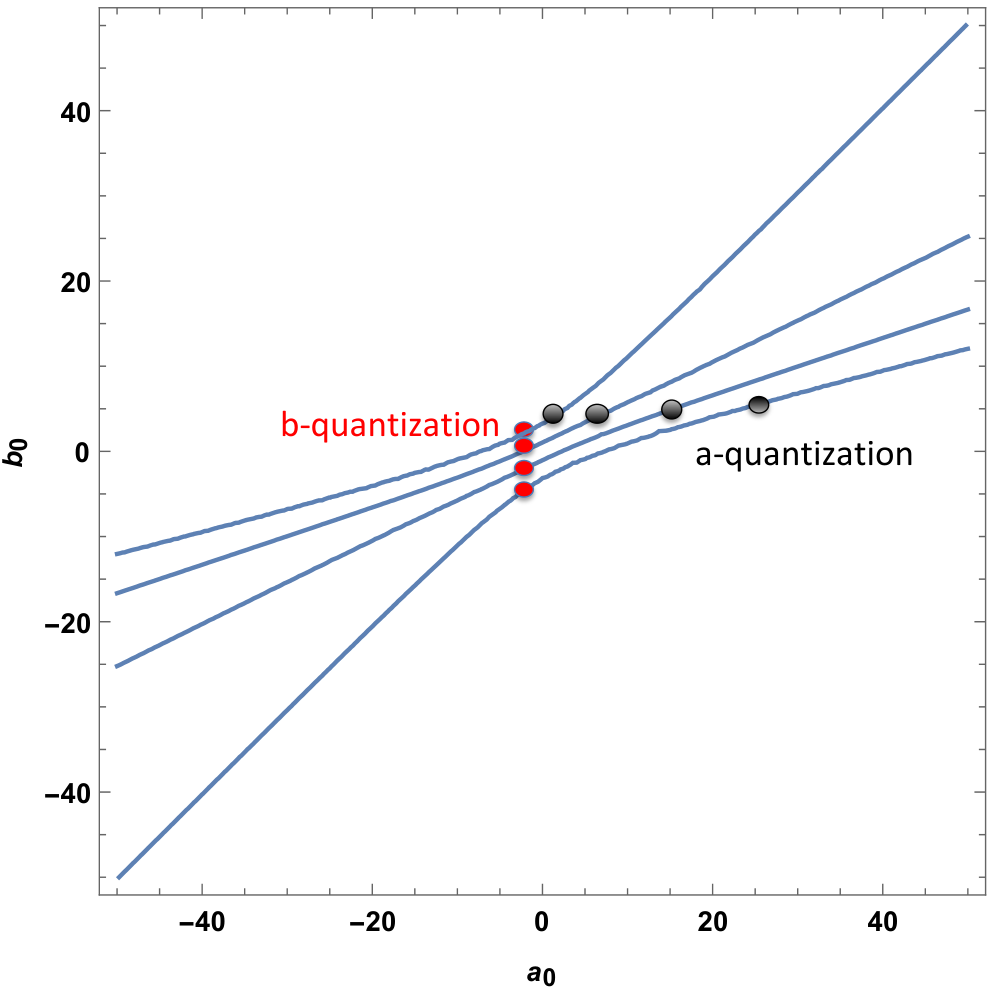
For general $N$, we can show that for large enough $a_{0},b_{0}$, ${\cal P}_{ㅜ+1}(a_{0},b_{0})=0$ gives following relation.

This means that for a given $b_{0}$, there are $N+1$ $a_{0}$’s for any $L$. This is also true for $|a_{0}|,|b_{0}|\leq{\cal O}(1)$ although we can not write down the explicitly. Similarly if we set $a_{0}=0$, the allowed values of $b_{0}$ are given by the crossing points of $N+1$ branches of the ${\cal P}_{N+1}=0$ with the vertical line $a_{0}=0$. We call such fixing $b$-quantization. See figure .

Such extra quantization is a consequence of the Heun’s equation. As we have seen before explicitly, for the hypergeometric equations, the the three term recurrence relation is reduced to two term one after factoring out the asymptotic form so that we need to fine tune only one parameter, the energy, to have a polynomial solution. For the Heun’s equation, its higher singularity requests higher regularity: the three term recurrence relation is not reduced to the two term one, which in turn request an extra quantization of system parameter apart from the energy eigenvalue.

Notice that due to the $N,L$ dependence of $b_{0}$, the spectrum $\mathcal{E}$ is NOT linear in $N$ anymore. Notice also that for $a$-quantization, $\mathcal{E}$ is linear in $N,L$ and does not depend on a quantized value of $a_{0}$ as far as $a_{0}$ is actually given by one of those quantized value that depends on $N$, $L$ and $b_{0}$. Table 1 tells us all possible roots of $a_{0}$’s for each $L$ when $N=4$ and $b_{0}=1$. Similarly, Table 2 shows us all possible roots of $a_{0}$’s for each $L$ when $N=5$ and $b_{0}=1$. As you can see easily from the table, most of the quantized values are in the linear regime where $a_{0}\approx(L+1+K)b_{0}$.

From the explicit calculation, we found the following pattern: List N+1 $a_{0}$ in the increasing order such that $a_{0K}$ is $K$-th one, $K=0,1,\cdots,N$. Then the polynomial solution for the $a_{0K}$ has $K$ nodes. The number of nodes does not depend on $L$.

Figs. 2(a) shows that polynomial $y_{4}$ with $a_{0K}$, $K=0,1,2,3,4$ has $K$ nodes in $N=4$ in the region $\rho>0$. We fixed $L=0$ and $b_{0}=1$. Figs. 2(b) shows that polynomials $y_{5}$ with $a_{03}$ has 3 nodes in $N=5$ independent of the value of $L=0,1,2,3,4,5$. There are two nodes in the unphysical region $\rho<0$.

5. Spectrum for nonzero quark mass: We have seen that two very different models lead to the same Heun’s equation. The spectrum of the Lichtenberg bag model for $m_{q}=0$ was obtained in Gursey and it is linear:

On the other hand, for $m_{q}\neq 0$, $b$ can not be an arbitrary value. It is determined by $b$-quantization because the parameter $a=0$. The value of $b$ for given $N,L$ was determined numerically Bag2019 and given by:

For odd $N$,

For even $N$,

By inserting eq(27) and eq(28) to eq(26), we see that not only the spectrum is highly nonlinear in $N,L$ but also the string tension is vanishingly small in the limit of $m_{q}\to 0$, which is inconsistent with the nature.

From the correspondence of two system given in eq(12), we can read off the spectrum of holographic model from that of the bag model by replacing

Exactly parallel comment for the bag model can be applied to the spectrum.

6. Summary and Discussion:

In this paper, we considered a holographic model where the confinement is consequence of the non-zero quark condensate $M$, so that $M$ play the role of the order parameter for the confinement transition as well as that for the chiral transition. We also showed that the equation of motion of our holographic model can be mapped to the Lichtenberg model. The quark mass triggers the change of the singularity type from the hypergeometric type to Heun’s type. The Regge trajectory appears only at the zero current quark mass limit where higher singularity disappears.

Before we finish, we discuss a similar model in $AdS_{5}$. The scalar solution in AdS5 with $m_{\Phi}^{2}=-4$ is

If the quark mass $M_{0}$ vanishes, we still have $\Phi={M}z^{2}$, which is necessary power in $z$ to give linear confinement. Therefore in this model, exactly the same calculation leads to the same result of AdS4 model. However, there is one subtlety here. $m_{\Phi}^{2}=2(2-4)=-4$ follows from the assumption that the dimension of $\langle\bar{q}q\rangle$ is $\Delta=2$, while its value for the free theory is 3 for 3+1 dimensional boundary theory. Therefore for our senario to work, we need anomalous dimension $\gamma=-1$ In 2+1 dimension, on the other hand, we can simply use the $m_{\Phi}^{2}=-2$ for $\Delta=2$, which is the reason why we used $AdS_{4}$ model in the main text.

References

- (1) E. V. Shuryak, “The QCD vacuum, hadrons and the superdense matter,” World Sci. Lect. Notes Phys. 71, 1 (2004). doi:10.1142/5367
- (2) K. Yagi, T. Hatsuda and Y. Miake, “Quark-gluon plasma: From big bang to little bang,” Camb. Monogr. Part. Phys. Nucl. Phys. Cosmol. 23, 1 (2005).
- (3) S. Mandelstam, Vortices and Quark Confinement in Nonabelian Gauge Theories, Phys. Rept. 23 (1976) 245–249.
- (4) G. ’t Hooft, Gauge Theory for Strong Interactions, in New Phenomena in Subnuclear Physics: Proceedings, International School of Subnuclear Physics, Erice, Sicily, Jul 11-Aug 1 1975. Part A, p. 0261, 1975.
- (5) Y. S. Choun and S. J. Sin, “Chiral symmetry and Heun’s equation,” arXiv:1909.07215 [hep-ph].
- (6) Lichtenberg, D. B., Namgung, W., Predazzi, E. and Wills,J. G., “Baryon masses in a relativistic quark-diquark model,” Phys. Lett. 48, 1653(1982).
- (7) Gürsey, F., Comments on hardronic mass formulae, in A. Das., ed., From Symmetries to Strings: Forty Years of Rochester Conferences, World Scientific, Singapore, (1990).
- (8) D. B. Kaplan, J.-W. Lee, D. T. Son and M. A. Stephanov, Conformality Lost, Phys. Rev. D80 (2009) 125005, [0905.4752].
- (9) E. Oh and S. J. Sin, “Holographic Abelian Higgs model and the Linear confinement,” arXiv:1909.13801 [hep-ph].
- (10) A. Karch, E. Katz, D. T. Son and M. A. Stephanov, Linear confinement and AdS/QCD, Phys. Rev. D74 (2006) 015005, [hep-ph/0602229].
- (11) R. Argurio, A. Marzolla, A. Mezzalira and D. Musso, JHEP 1603, 012 (2016) doi:10.1007/JHEP03(2016)012 [arXiv:1512.03750 [hep-th]].
- (12) NIST Digital Library of Mathematical Functions, “Confluent Forms of Heun Equation,” http://dlmf.nist.gov/31.12
- (13) Ronveaux, A., Heun Differential Equations, Oxford University Press, (1995).
- (14) Slavyanov, S. Yu., Lay W. Special Functions: A Unified Theory Based on Singularities, Oxford Mathematical Monographs, Oxford University Press, Oxford, (2000).