Splitting Steepest Descent for Growing Neural Architectures
Abstract
We develop a progressive training approach for neural networks which adaptively grows the network structure by splitting existing neurons to multiple off-springs. By leveraging a functional steepest descent idea, we derive a simple criterion for deciding the best subset of neurons to split and a splitting gradient for optimally updating the off-springs. Theoretically, our splitting strategy is a second-order functional steepest descent for escaping saddle points in an -Wasserstein metric space, on which the standard parametric gradient descent is a first-order steepest descent. Our method provides a new practical approach for optimizing neural network structures, especially for learning lightweight neural architectures in resource-constrained settings.
1 Introduction
Deep neural networks (DNNs) have achieved remarkable empirical successes recently. However, efficient and automatic optimization of model architectures remains to be a key challenge. Compared with parameter optimization which has been well addressed by gradient-based methods (a.k.a. back-propagation), optimizing model structures involves significantly more challenging discrete optimization with large search spaces and high evaluation cost. Although there have been rapid progresses recently, designing the best architectures still requires a lot of expert knowledge and trial-and-errors for most practical tasks.
This work targets extending the power of gradient descent to the domain of model structure optimization of neural networks. In particular, we consider the problem of progressively growing a neural network by “splitting” existing neurons into several “off-springs”, and develop a simple and practical approach for deciding the best subset of neurons to split and how to split them, adaptively based on the existing model structure. We derive the optimal splitting strategies by considering the steepest descent of the loss when the off-springs are infinitesimally close to the original neurons, yielding a splitting steepest descent that monotonically decreases the loss in the space of model structures.
Our main method, shown in Algorithm 1, alternates between a standard parametric descent phase in which we update the parameters to minimize the loss with a fixed model structure, and a splitting phase in which we update the model structures by splitting neurons. The splitting phase is triggered when no further improvement can be made by only updating parameters, and allow us to escape the parametric local optima by augmenting the neural network in a locally optimal fashion. Theoretically, these two phases can be viewed as performing functional steepest descent on an -Wasserstein metric space, in which the splitting phase is a second-order descent for escaping saddle points in the functional space, while the parametric gradient descent corresponds to a first-order descent. Empirically, our algorithm is simple and practical, and provides a promising tool for many challenging problems, especially for learning lightweight and energy-efficient neural architectures for resource-constrained settings.
Related Works
The idea of progressively growing neural networks by node splitting is not new, but previous works are mostly based on heuristic or purely random splitting strategies (Wynne-Jones 1992; Chen et al. 2016, e.g.,). A different approach for progressive training is the Frank-Wolfe or gradient boosting based strategies (Schwenk & Bengio 2000; Bengio et al. 2006; Bach 2017, e.g.,), which iteratively add new neurons derived from functional conditional gradient, while keeping the previous neurons fixed. However, these methods are not suitable for large scale settings, because adding each neuron requires to solve a difficult non-convex optimization problem, and keeping the previous neurons fixed prevents us from correcting the mistakes made in earlier iterations. A practical alternative of Frank-Wolfe is to simply add new randomly initialized neurons and co-optimize the new and old neurons together. However, random initialization does not allow us to leverage the information of the existing model and takes more time to converge. In contrast, splitting neurons from the existing network allows us to inherent the knowledge from the existing model (see Chen et al. 2016), and is faster to converge in settings like continual learning, when the previous model is not far away from the optimal solution.
An opposite direction of progressive training is to prune large pre-trained neural networks to obtain compact network structures (Han et al. 2016; Li et al. 2017; Liu et al. 2017, e.g.,). In comparison, our splitting method requires no large pre-trained models and is more suitable for learning very small network structures, which is of critical importance for resource-constrained settings like mobile devices and Internet of things. As shown in our experiments, our method can outperform existing pruning methods in learning more accurate models with small model sizes.
More broadly, there has been a series of recent works on neural architecture search, based on various strategies from combinatorial optimization, including reinforcement learning (RL) (Pham et al. 2018; Cai et al. 2018; Zoph & Le 2017, e.g.,), evolutionary algorithms (EA) (Stanley & Miikkulainen 2002; Real et al. 2018, e.g.,), and continuous relaxation (Liu et al. 2019a; Xie et al. 2018, e.g.,). However, these general-purpose black-box optimization methods do not efficient leverage the inherent geometric structure of the loss landscape, and are highly computationally expensive due to the need of evaluating the candidate architectures based on inner training loops.
Background: Steepest Descent and Saddle Points
Stochastic gradient descent is the driving horse for solving large scale optimization in machine learning and deep learning. Gradient descent can be viewed as a steepest descent procedure that iteratively improves the solution by following the direction that maximally decreases the loss function within a small neighborhood of the previous solution. Specifically, for minimizing a loss function , each iteration of steepest descent updates the parameter via , where is a small step size and is an update direction chosen to maximally decrease the loss of the updated parameter under a norm constraint , where denotes the Euclidean norm. When and is infinitesimal, the optimal descent direction equals the negative gradient direction, that is, , yielding a descent of . At a critical point with a zero gradient (), the steepest descent direction depends on the spectrum of the Hessian matrix . Denote by the minimum eigenvalue of and its associated eigenvector. When , the point is a stable local minimum and no further improvement can be made in the infinitesimal neighborhood. When , the point is a saddle point or local maximum, and the steepest descent direction equals the eigenvector , which yields an decrease on the loss.11 1 The property of the case when depends on higher order information. In practice, it has been shown that there is no need to explicitly calculate the negative eigenvalue direction, because saddle points and local maxima are unstable and can be escaped by using gradient descent with random initialization or stochastic noise (Lee et al. 2016; Jin et al. 2017, e.g.,).
2 Splitting Neurons Using Steepest Descent
We introduce our main method in this section. We first illustrate the idea with the simple case of splitting a single neuron in Section 2.1, and then consider the more general case of simultaneously splitting multiple neurons in deep networks in Section 2.2, which yields our main progressive training algorithm (Algorithm 1). Section 2.3 draws a theoretical discussion and interpret our procedure as a functional steepest descent of the distribution of the neuron weights under the -Wasserstein metric.
2.1 Splitting a Single Neuron
Let be a neuron inside a neural network that we want to learn from data, where is the parameter of the neuron and its input variable. Assume the loss of has a general form of
| (1) |
where is a data distribution, and is a map determined by the overall loss function. The parameters of the other parts of the network are assumed to be fixed or optimized using standard procedures and are omitted for notation convenience.
Standard gradient descent can only yield parametric updates of . We introduce a generalized steepest descent procedure that allows us to incrementally grow the neural network by gradually introducing new neurons, achieved by “splitting” the existing neurons into multiple copies in a (locally) optimal fashion derived using ideas from steepest descent idea.
In particular, we split into off-springs , and replace the neuron with a weighted sum of the off-spring neurons , where is a set of positive weights assigned on the off-springs, and satisfies , . This yields an augmented loss function on and :
| (2) |
A key property of this construction is that it introduces a smooth change on the loss function when the off-springs are close to the original parameter : when , , the augmented network and loss are equivalent to the original ones, that is, , where denotes the vector consisting of all ones; when all the are within an infinitesimal neighborhood of , it yields an infinitesimal change on the loss, with which a steepest descent can be derive.
Formally, consider the set of splitting schemes whose off-springs are -close to the original neuron:
We want to decide the optimal to maximize the decrease of loss , when the step size is infinitesimal. Although this appears to be an infinite dimensional optimization because is allowed to be arbitrarily large, we show that the optimal choice is achieved with either (no splitting) or (splitting into two off-springs), with uniform weights . Whether a neuron should be split ( or ) and the optimal values of the off-springs are decided by the minimum eigenvalue and eigenvector of a splitting matrix, which plays a role similar to Hessian matrix for deciding saddle points.
Definition 2.1 (Splitting Matrix).
For in (1), its splitting matrix is defined as
| (3) |
We call the minimum eigenvalue of the splitting index of , and the eigenvector related to the splitting gradient of .
The splitting matrix is a symmetric “semi-Hessian” matrix that involves the first derivative , and the second derivative of . It is useful to compare it with the typical gradient and Hessian matrix of :
where is the outer product. The splitting matrix differs from the gradient in replacing with the second-order derivative , and differs from the Hessian matrix in missing an extra term . We should point out that is the “easier part” of the Hessian matrix, because the second-order derivative of the individual neuron is much simpler than the second-order derivative of “everything else”, which appears in the extra term . In addition, as we show in Section 2.2, is block diagonal in terms of multiple neurons, which is crucial for enabling practical computational algorithm.
It is useful to decompose each into , where is an average displacement vector shared by all copies, and is the splitting vector associated with , and satisfies (which implies ). It turns out that the change of loss naturally decomposes into two terms that reflect the effects of the average displacement and splitting, respectively.
Theorem 2.2.
Assume with and . For and in (1) and (2), assume has bounded third order derivatives w.r.t. . We have
| (4) |
where the change of loss is decomposed into two terms: the first term is the effect of the average displacement , and it is equivalent to applying the standard parametric update on . The second term is the change of the loss caused by the splitting vectors . It depends on only through the splitting matrix .
Therefore, the optimal average displacement should be decided by standard parametric steepest (gradient) descent, which yields a typical decrease of loss at non-stationary points. In comparison, the splitting term is always , which is much smaller. Given that introducing new neurons increases model size, splitting should not be preferred unless it is impossible to achieve an gain with pure parametric updates that do not increase the model size. Therefore, it is motivated to introduce splitting only at stable local minima, when the optimal equals zero and no further improvement is possible with (infinitesimal) regular parametric descent on . In this case, we only need to minimize the splitting term to decide the optimal splitting strategy, which is shown in the following theorem.
Theorem 2.3.
a) If the splitting matrix is positive definite, that is, , we have for any and , and hence no infinitesimal splitting can decrease the loss. We call that is splitting stable in this case.
b) If , an optimal splitting strategy that minimizes subject to is
| and |
where , called the splitting gradient, is the eigenvector related to . Here we split the neuron into two copies of equal weights, and update each copy with the splitting gradient. The change of loss obtained in this case is .
Remark
The splitting stability () does not necessarily ensure the standard parametric stability of (i.e., ), except when is convex which ensures (see Definition 2.1). If both and hold, the loss can not be improved by any local update or splitting, no matter how many off-springs are allowed. Since stochastic gradient descent guarantees to escape unstable stationary points (Lee et al. 2016; Jin et al. 2017), we only need to calculate to decide the splitting stability in practice.
2.2 Splitting Deep Neural Networks
In practice, we need to split multiple neurons simultaneously, which may be of different types, or locate in different layers of a deep neural network. The key questions are if the optimal splitting strategies of different neurons influence each other in some way, and how to compare the gain of splitting different neurons and select the best subset of neurons to split under a budget constraint.
It turns out the answers are simple. We show that the change of loss caused by splitting a set of neurons is simply the sum of the splitting terms of the individual neurons. Therefore, we can calculate the splitting matrix of each neuron independently without considering the other neurons, and compare the “splitting desirability” of the different neurons by their minimum eigenvalues (splitting indexes). This motivates our main algorithm (Algorithm 1), in which we progressively split the neurons with the most negative splitting indexes following their own splitting gradients. Since the neurons can be in different layers and of different types, this provides an adaptive way to grow neural network structures to fit best with data.
| where |
To set up the notation, let be the parameters of a set of neurons (or any duplicable sub-structures) in a large neural network, where is the parameter of the -th neuron. Assume we split into copies , with weights satisfying and , . Denote by and the loss function of the original and augmented networks, respectively. It is hard to specify the actual expression of the loss functions in general cases, but it is sufficient to know that depends on each only through the output of its related neuron,
| (5) |
where denotes the activation function of neuron , and and denote the parts of the loss that connect to the input and output of neuron , respectively, both of which depend on the other parameters in some complex way. Similarly, the augmented loss satisfies
| (6) |
where , and , are the augmented variants of , , respectively.
Interestingly, although each equation in (5) and (6) only provides a partial specification of the loss function of deep neural nets, they together are sufficient to establish the following key extension of Theorem 2.2 to the case of multiple neurons.
Theorem 2.4.
Under the setting above, assume for , where denotes the average displacement vector on , and is the -th splitting vector of , with . Assume has bounded third order derivatives w.r.t. . We have
where the effect of average displacement is again equivalent to that of the corresponding parametric update ; the splitting effect equals the sum of the individual splitting terms , which depends on the splitting matrix of neuron ,
| (7) |
The important implication of Theorem 2.4 is that there is no crossing term in the splitting matrix, unlike the standard Hessian matrix. Therefore, the splitting effect of an individual neuron only depends on its own splitting matrix and can be evaluated individually; the splitting effects of different neurons can be compared using their splitting indexes, allowing us to decide the best subset of neurons to split when a maximum number constraint is imposed. As shown in Algorithm 1, we decide a maximum number of neurons to split at each iteration, and a threshold of splitting index, and split the neurons whose splitting indexes are ranked in top and smaller than .
Computational Efficiency
The computational cost of exactly evaluating all the splitting indexes and gradients on a data instance is , where is the number of neurons and is the number of the parameters of each neuron. Note that this is much better than evaluating the Hessian matrix, which costs , where is the total number of parameters (e.g., ). In practice, is not excessively large or can be controlled by identifying a subset of important neurons to split. Further computational speedup can be obtained by using efficient gradient-based large scale eigen-computation methods, which we investigate in future work.
2.3 Splitting as -Wasserstein Steepest Descent
We present a functional aspect of our approach, in which we frame the co-optimization of the neural parameters and structures into a functional optimization in the space of distributions of the neuron weights, and show that our splitting strategy can be viewed as a second-order descent for escaping saddle points in the -Wasserstein space of distributions, while the standard parametric gradient descent corresponds to a first-order descent in the same space.
We illustrate our theory using the single neuron case in Section 2.1. Consider the augmented loss in (2). Because the off-springs of the neuron are exchangeable, we can equivalently represent as a functional of the empirical measure of the off-springs,
| (8) |
where denotes the delta measure on and is the functional representation of . The idea is to optimize in the space of probability distributions (or measures) using a functional steepest descent. To do so, a notion of distance on the space of distributions need to be decided. We consider the -Wasserstein metric,
| (9) |
where denotes the set of probability measures whose first and second marginals are and , respectively, and can be viewed as describing a transport plan from to . We obtain the -Wasserstein metric in the limit when , in which case the -norm reduces to an esssup norm, that is,
where the notation denotes the smallest number such that the set has zero probability under . See more discussion in Villani 2008 and Appendix A.2.
The -Wasserstein metric yields a natural connection to node splitting. For each , the conditional distribution represents the distribution of points transported from , which can be viewed as the off-springs of in the context of node splitting. If , it means that can be obtained from splitting such that all the off-springs are -close, i.e., . This is consistent with the augmented neighborhood introduced in Section 2.1, except that here can be an absolutely continuous distribution, representing a continuously infinite number of off-springs; but this yields no practical difference because any distribution can be approximated arbitrarily close using a countable number of particles. Note that -Wasserstein metrics with finite are not suitable for our purpose because with does not ensure for all and .
Similar to the steepest descent on the Euclidean space, the -Wasserstein steepest descent on should iteratively find new points that maximize the decrease of loss in an -ball of the current points. Define
We are ready to show the connection of Algorithm 1 to the -Wasserstein steepest descent.
Theorem 2.5.
Consider the and in (2) and (8), connected with . Define and with , which are related to the gradient and splitting matrices of , respectively. Assume has bounded third order derivatives w.r.t. .
a) If is on a non-stationary point w.r.t. , then the steepest descent of is achieved by moving all the particles of with gradient descent on , that is,
where denotes the distribution of when .
b) If reaches a stable local optima w.r.t. , the steepest descent on is splitting each neuron with into two copies of equal weights following their minimum eigenvectors, while keeping the remaining neurons to be unchanged. Precisely, denote by the distribution obtained in this way, we have
where we have .
Remark
There has been a line of theoretical works on analyzing gradient-based learning of neural networks via -Wasserstein gradient flow by considering the mean field limit when the number of neurons goes to infinite (Mei et al. 2018; Chizat & Bach 2018, e.g.,). These analysis focus on the first-order descent on the -Wasserstein space as a theoretical tool for understanding the behavior of gradient descent on overparameterized neural networks. Our framework is significant different, since we mainly consider the second-order descent on the -Wasserstein space, and the case of finite number of neurons in order to derive practical algorithms.
3 Experiments
We test our method on both toy and realistic tasks, including learning interpretable neural networks, architecture search for image classification and energy-efficient keyword spotting. Due to limited space, many of the detailed settings are shown in Appendix, in which we also include additional results on distribution approximation (Appendix B.5).
| Eigenvalues Loss decrease | Training Loss | ||
| (a) | (b) | (c) Angle | (d) #Iteration |
Toy RBF Neural Networks
We apply our method to learn a one-dimensional RBF neural network shown in Figure 1a. See Appendix B.1 for details of the setting. We start with a small neural network with neuron and gradually increase the model size by splitting neurons. Figure 1a shows that we almost recover the true function as we split up to neurons. Figure 1b shows the top five eigenvalues and the decrease of loss when we split neurons to neurons; we can see that the eigenvalue and loss decrease correlate linearly, confirming our results in Theorem 2.4. Figure 1c shows the decrease of the loss when we split the top one neuron following the direction with different angles from the minimum eigenvector at . We can see that the decrease of the loss is maximized when the splitting direction aligns with the eigenvector, consistent with our theory. In Figure 1d, we compare with different baselines of progressive training, including Random Split, splitting a randomly chosen neuron with a random direction; New Initialization, adding a new neuron with randomly initialized weights and co-optimization it with previous neurons; Gradient Boosting, adding new neurons with Frank-Wolfe algorithm while fixing the previous neurons; Baseline (scratch), training a network of size from scratch. Figure 1d shows our method yields the best result.
Learning Interpretable Neural Networks
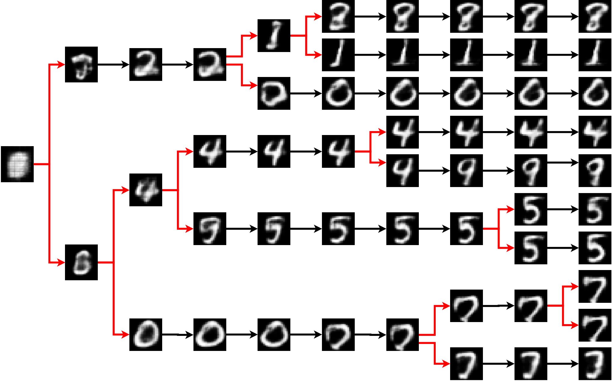
To visualize the dynamics of the splitting process, we apply our method to incrementally train an interpretable neural network designed by Li et al. 2018, which contains a “prototype layer” whose weights are enforced to be similar to realistic images to encourage interpretablity. See Appendix B.2 and Li et al. 2018 for more detailed settings. We apply our method to split the prototype layer starting from a single neuron on MNIST, and show in Figure 2 the evolutionary tree of the neurons in our splitting process. We can see that the blurry (and hence less interpretable) prototypes tend to be selected and split into two off-springs that are similar yet more interpretable. Figure 2 (b) shows the decrease of loss when we split each of the five neurons at the 5-th step (with the decrease of loss measured at the local optima reached dafter splitting); we find that the eigenvalue correlates well with the decrease of loss and the interpretablity of the neurons. The complete evolutionary tree and quantitative comparison with baselines are shown in Appendix B.2.
 |
Eigenvalues
 Loss decrease
|
| (a) | (b) |
Lightweight Neural Architectures for Image Classification
We investigate the effectiveness of our methods in learning small and efficient network structures for image classification. We experiment with two popular deep neural architectures, MobileNet (Howard et al. 2017) and VGG19 (Simonyan & Zisserman 2015). In both cases, we start with a relatively small network and gradually grow the network by splitting the convolution filters following Algorithm 1. See Appendix B.3 for more details of the setting. Because there is no other off-the-shelf progressive growing algorithm that can adaptively decide the neural architectures like our method, we compare with pruning methods, which follow the opposite direction of gradually removing neurons starting from a large pre-trained network. We test two state-of-the-art pruning methods, including batch-normalization-based pruning (Bn-prune) (Liu et al. 2017) and L1-based pruning (L1-prune) (Li et al. 2017). As shown in Figure 3a-b, our splitting method yields higher accuracy with similar model sizes. This is surprising and significant, because the pruning methods leverage the knowledge from a large pre-train model, while our method does not.
To further test the effect of architecture learning in both splitting and pruning methods, we test another setting in which we discard the weights of the neurons and retain the whole network starting from a random initialization, under the structure obtained from splitting or pruning at each iteration. As shown in Figure 3c-d, the results of retraining is comparable with (or better than) the result of successive finetuning in Figure 3a-b, which is consistent with the findings in Liu et al. 2019b. Meanwhile, our splitting method still outperforms both Bn-prune and L1-prune.
| MobileNet (finetune) | VGG19 (finetune) | MobileNet (retrain) | VGG19 (retrain) |
| Test Accuracy | |||
| (a) Ratio | (b) Ratio | (c) Ratio | (d) Ratio |
Resource-Efficient Keyword Spotting on Edge Devices
Keyword spotting systems aim to detect a particular keyword from a continuous stream of audio. It is typically deployed on energy-constrained edge devices and requires real-time response and high accuracy for good user experience. This casts a key challenge of constructing efficient and lightweight neural architectures. We apply our method to solve this problem, by splitting a small model (a compact version of DS-CNN) obtained from Zhang et al. 2017. See Appendix B.4 for detailed settings.
Table 1 shows the results on the Google speech commands benchmark dataset (Warden 2018), in which our method achieves significantly higher accuracy than the best model (DS-CNN) found by Zhang et al. 2017, while having 31% less parameters and Flops. Figure 4 shows further comparison with Bn-prune (Liu et al. 2017), which is again inferior to our method.
| Method | Acc | Params (K) | Ops (M) |
|---|---|---|---|
| DNN | 86.94 | 495.7 | 1.0 |
| CNN | 92.64 | 476.7 | 25.3 |
| BasicLSTM | 93.62 | 492.6 | 47.9 |
| LSTM | 94.11 | 495.8 | 48.4 |
| GRU | 94.72 | 498.0 | 48.4 |
| CRNN | 94.21 | 485.0 | 19.3 |
| DS-CNN | 94.85 | 413.7 | 56.9 |
| Ours | 95.36 | 282.6 | 39.2 |
| Test Accuracy | |
| #Params | #Ops |
4 Conclusion
We present a simple approach for progressively training neural networks via neuron splitting. Our approach highlights a novel view of neural structure optimization as continuous functional optimization, and yields a practical procedure with broad applications. For future work, we will further investigate fast gradient descent based approximation of large scale eigen-computation and more theoretical analysis, extensions and applications of our approach.
Acknowledgement
This work is supported in part by NSF CRII 1830161 and NSF CAREER 1846421. We would like to acknowledge Google Cloud and Amazon Web Services (AWS) for their support.
References
- Bach (2017) Bach, Francis. Breaking the curse of dimensionality with convex neural networks. Journal of Machine Learning Research, 18(19):1–53, 2017.
- Bach et al. (2012) Bach, Francis, Lacoste-Julien, Simon, and Obozinski, Guillaume. On the equivalence between herding and conditional gradient algorithms. In Proceedings of the 29th International Coference on International Conference on Machine Learning, pp. 1355–1362. Omnipress, 2012.
- Bengio et al. (2006) Bengio, Yoshua, Roux, Nicolas L, Vincent, Pascal, Delalleau, Olivier, and Marcotte, Patrice. Convex neural networks. In Advances in neural information processing systems, pp. 123–130, 2006.
- Cai et al. (2018) Cai, Han, Zhu, Ligeng, and Han, Song. Proxylessnas: Direct neural architecture search on target task and hardware. In International Conference on Learning Representation, 2018.
- Chen et al. (2016) Chen, Tianqi, Goodfellow, Ian, and Shlens, Jonathon. Net2net: Accelerating learning via knowledge transfer. In International Conference on Learning Representations, 2016.
- Chen et al. (2010) Chen, Yutian, Welling, Max, and Smola, Alex. Super-samples from kernel herding. In Conference on Uncertainty in Artificial Intelligence (UAI), 2010.
- Chizat & Bach (2018) Chizat, Lenaic and Bach, Francis. On the global convergence of gradient descent for over-parameterized models using optimal transport. In Advances in neural information processing systems, pp. 3036–3046, 2018.
- Gretton et al. (2012) Gretton, Arthur, Borgwardt, Karsten M, Rasch, Malte J, Schölkopf, Bernhard, and Smola, Alexander. A kernel two-sample test. Journal of Machine Learning Research, 13(Mar):723–773, 2012.
- Han et al. (2016) Han, Song, Mao, Huizi, and Dally, William J. Deep compression: Compressing deep neural networks with pruning, trained quantization and huffman coding. International Conference on Learning Representations, 2016.
- Howard et al. (2017) Howard, Andrew G, Zhu, Menglong, Chen, Bo, Kalenichenko, Dmitry, Wang, Weijun, Weyand, Tobias, Andreetto, Marco, and Adam, Hartwig. Mobilenets: Efficient convolutional neural networks for mobile vision applications. arXiv preprint arXiv:1704.04861, 2017.
- Jin et al. (2017) Jin, Chi, Ge, Rong, Netrapalli, Praneeth, Kakade, Sham M, and Jordan, Michael I. How to escape saddle points efficiently. In Proceedings of the 34th International Conference on Machine Learning-Volume 70, pp. 1724–1732. JMLR. org, 2017.
- Lee et al. (2016) Lee, Jason D, Simchowitz, Max, Jordan, Michael I, and Recht, Benjamin. Gradient descent only converges to minimizers. In Conference on learning theory, pp. 1246–1257, 2016.
- Li et al. (2017) Li, Hao, Kadav, Asim, Durdanovic, Igor, Samet, Hanan, and Graf, Hans Peter. Pruning filters for efficient convnets. International Conference on Learning Representations, 2017.
- Li et al. (2018) Li, Oscar, Liu, Hao, Chen, Chaofan, and Rudin, Cynthia. Deep learning for case-based reasoning through prototypes: A neural network that explains its predictions. In Thirty-Second AAAI Conference on Artificial Intelligence, 2018.
- Liu et al. (2019a) Liu, Hanxiao, Simonyan, Karen, and Yang, Yiming. Darts: Differentiable architecture search. International Conference on Learning Representations, 2019a.
- Liu et al. (2017) Liu, Zhuang, Li, Jianguo, Shen, Zhiqiang, Huang, Gao, Yan, Shoumeng, and Zhang, Changshui. Learning efficient convolutional networks through network slimming. In Proceedings of the IEEE International Conference on Computer Vision, pp. 2736–2744, 2017.
- Liu et al. (2019b) Liu, Zhuang, Sun, Mingjie, Zhou, Tinghui, Huang, Gao, and Darrell, Trevor. Rethinking the value of network pruning. International Conference on Learning Representations, 2019b.
- Mei et al. (2018) Mei, Song, Montanari, Andrea, and Nguyen, Phan-Minh. A mean field view of the landscape of two-layers neural networks. Proceedings of the National Academy of Sciences of USA, 2018.
- Pham et al. (2018) Pham, Hieu, Guan, Melody, Zoph, Barret, Le, Quoc, and Dean, Jeff. Efficient neural architecture search via parameter sharing. In International Conference on Machine Learning, pp. 4092–4101, 2018.
- Rahimi & Recht (2007) Rahimi, Ali and Recht, Benjamin. Random features for large-scale kernel machines. In Advances in Neural Information Processing Systems, pp. 1177–1184, 2007.
- Real et al. (2018) Real, Esteban, Aggarwal, Alok, Huang, Yanping, and Le, Quoc V. Regularized evolution for image classifier architecture search. ICML AutoML Workshop, 2018.
- Schwenk & Bengio (2000) Schwenk, Holger and Bengio, Yoshua. Boosting neural networks. Neural computation, 12(8):1869–1887, 2000.
- Simonyan & Zisserman (2015) Simonyan, Karen and Zisserman, Andrew. Very deep convolutional networks for large-scale image recognition. International Conference on Learning Representations, 2015.
- Stanley & Miikkulainen (2002) Stanley, Kenneth O and Miikkulainen, Risto. Evolving neural networks through augmenting topologies. Evolutionary computation, 10(2):99–127, 2002.
- Villani (2008) Villani, Cédric. Optimal transport: old and new, volume 338. Springer Science & Business Media, 2008.
- Warden (2018) Warden, Pete. Speech commands: A dataset for limited-vocabulary speech recognition. arXiv preprint arXiv:1804.03209, 2018.
- Wynne-Jones (1992) Wynne-Jones, Mike. Node splitting: A constructive algorithm for feed-forward neural networks. In Advances in neural information processing systems, pp. 1072–1079, 1992.
- Xie et al. (2018) Xie, Sirui, Zheng, Hehui, Liu, Chunxiao, and Lin, Liang. SNAS: stochastic neural architecture search. International Conference on Learning Representations, 2018.
- Zhang et al. (2017) Zhang, Yundong, Suda, Naveen, Lai, Liangzhen, and Chandra, Vikas. Hello edge: Keyword spotting on microcontrollers. arXiv preprint arXiv:1711.07128, 2017.
- Zoph & Le (2017) Zoph, Barret and Le, Quoc V. Neural architecture search with reinforcement learning. International Conference on Learning Representations, 2017.
Appendix A Proofs
A.1 Proofs of Splitting Taylor Expansion
Proof of Theorem 2.2.
Taking the gradient of in (1) gives
where is the derivative of (which is a univariate function), and
When is split into , the augmented loss function is
where and The weights should satisfy and . In this way, we have when .
Taking the gradient of w.r.t. when , we have
Taking the second derivative, we get
where
Note that we have following this definition.
For , we have
For , assume , and define to be the average displacement. Therefore, . Using the Taylor expansion of w.r.t. at , we have
This completes the proof. ∎
Proof of Theorem 2.3.
Recall that
with , and . Since , it is obvious that
On the other hand, this lower bound is achieved by setting , and This completes the proof. ∎
Proof of Theorem 2.4.
Step 1: We first consider the case with no average displacement, that is, . In this case, Lemma A.1 below gives
| (10) |
where denotes the augmented parameters obtained when we only split the -th neuron, while keeping all the neurons unchanged. Applying Theorem 2.2, we have for each ,
Combining this with (10) yields the result.
Step 2: We now consider the more general case when . Let . Applying the result above on , we have
where Therefore,
where This completes the proof. ∎
Lemma A.1.
Let be the parameters of neurons. Recall that we assume is split into off-springs with parameters and weights , which satisfies . Let , where is the perturbation on the -th off-spring of the -th neuron. Assume , that is, the average displacement of all the neurons is zero.
Denote by the augmented parameters we obtained by only splitting the -th neuron while keeping all the other neurons unchanged, that is, we have for , and for all and . Assume the third order derivatives of are bounded. We have
Proof.
Define
By Taylor expansion,
It is obvious to see that the first order derivation equals zero because of the correction terms. Specifically,
For the second order derivation, define
For any , we have from (5) and (6) that
Therefore, we have
where only involves cross derivatives with , because all the terms with are cancelled due to the correction terms. ∎
A.2 Proofs of -Wasserstein Steepest Descent
Recall that -Wasserstein distance is
When , we obtain -Wasserstein distance,
| (11) |
where denotes essential supremum; it is the minimum value with .
In the proof, we denote by an optimal solution of in (11), that is,
is called an -Wasserstein optimal coupling of and . Denote by and the mean and covariance matrix of under , conditional on , that is,
It is natural to expect that we can upper bound the magnitude of both and by the -Wasserstein distance.
Lemma A.2.
Following the definition above, we have
almost surely for .
Proof.
We have
almost surely for . And
∎
Theorem A.3.
Define . For two distributions and and their -Wasserstein optimal coupling . We have
| (12) | ||||
Proof.
We write for convenience. Denote by and the first and second order derivatives of in terms of its first variable.
For , introduce , whose distribution is denoted by . We have and . Taking Taylor expansion of w.r.t. , we have
where is a number between and . We just need to calculate the derivatives. For the first order derivative, we have
where we used the derivation of .
For the second order derivative, we have
where we define . Denote by We have
This completes the proof. ∎
Theorem A.4.
For two distributions and , denote by their -Wasserstein optimal coupling, and and the mean and covariance matrix of under , conditional on , respectively. Denote by the distribution of when . We have
| (13) |
where The first and second terms capture the effect of displacement and splitting, respectively.
Proof of Theorem A.4.
We use for notation convenience. Denote by and the distribution of when . Recall that for , we have
| (14) |
| (15) |
Introduce . Denote by the distribution of . This gives and . We have
where is a number between and . We just need to evaluate these derivatives. For the first order derivative, we have
where the last step uses (14). Here denote the derivatives w.r.t. its first variables.
For the second order derivative, we have
| (16) | ||||
Further, we can show that , since when taking the third gradient, all the terms of the derivative are bounded by . Specifically, taking the derivative of the form of in (16) gives
Here we use the notation . This completes the proof. ∎
Proof of Theorem 2.5.
Following Theorem A.3, we have
For , we must have , and hence by Cauchy–Schwarz inequality. On the other hand, this minimum is achieved when . The only distribution that satisfies this condition is . This proves Theorem 2.5a.
For Theorem 2.5b, we need to use the result in Theorem A.4, which yields, in the case of stable local optima, that
Similar to the argument above, the minima should satisfy , where is the eigenvector of associated with its minimum eigenvalue. This corresponds to splitting into two copies with each weights with parameter when , or keep unchanged when . ∎
Appendix B Experimental Settings and Additional Results
B.1 Two-Layer RBF Neural network
We consider fitting a simple radial basis function (RBF) neural network of form
where and . For the ground truth, we set and sample the true values of parameters from , yielding the light blue curves shown in Figure 5. We generate a training data set by drawing from and set without noise, where denotes the true network we sampled. The network is trained by minimizing the mean square loss:
Mapping to (2), we have . We learn the function using our splitting method and other progressive training baselines, all starting from neuron. We add one additional neuron in each splitting/growing phase for all the methods. The parametric descent phase is performed using typical stochastic gradient descent until convergence. We stop the splitting process at for all the methods. Figure 5 shows curves learned by different methods with and neurons, respectively. Our method yields better approximation.
| (a) | (b) |
|---|
B.2 Learning Interpretable Neural Network
We provide more details on learning the interpretable neural network.
Setting
We adopt the interpretable neural architecture proposed in Li et al. 2018 as our testbed. Unlike standard black-box neural networks, this architecture contains a special prototype layer in the classifier, which includes a set of prototype neurons that are enforced to encode to realistic images for promoting interpretability. In this model, each input image is first mapped to a lower-dimensional representation based on its distance with a set of prototype vectors, where represents a prototype vector and is an encoder function. The prototype vectors are enforced to be interpretable in that they can be decoded to some realistic images; this is achieved in Li et al. 2018 by introducing a regularization term that minimizes the minimum square distance between the prototypes and the training data, that is, , where denotes the training dataset.
We apply our method to split the prototype neurons, by treating as the activation function. We use the MNIST dataset in our experiment. We visualize the prototype neurons we learned using the images that they encode, by feeding the prototype vectors into a decoder function jointly trained with the network. We use the same encoder and decoder architectures, as suggested in Li et al. 2018 and refer the reader to Li et al. 2018 for more implementation details. To better understand the splitting dynamics, we start with a small network with just one prototype neuron and gradually add more prototypes via splitting.
We compare our method with two baseline methods, New Initialization and Random Split, that also progressively grow the prototype layers starting from one prototype neuron. In New Initialization, we simply add one new prototype neuron with random initialization at each iteration. In Random Split, we randomly pick a prototype neuron to split and split it following its splitting gradient given by our splitting matrix. Figure 6 visualizes the full splitting/growing process of our method and the two baselines. We can see that our splitting method successfully identifies the most ambiguous (and least interpretable) prototype neurons to split at each iteration, and achieves the best final results.
| Optimal Split (Ours) |
 |
| Random Split |
 |
| New Initialization |
 |
B.3 Lightweight Neural Architectures for Image Classification
We describe details of our experiments on learning lightweight deep networks for image classification.
Dataset and Backbone Networks
We use the CIFAR-10 benchmark dataset. We adopt a standard data argumentation scheme (mirroring and shifting) that is widely used for this dataset (Liu et al. 2019b; Liu et al. 2017). The input images are normalized using channel means and standard derivations. We use two popular deep neural architectures as our testbed, MobileNet (Howard et al. 2017) and VGG19 (Simonyan & Zisserman 2015).
Training Settings
We treat the filters as the neurons to split for convolutional neural networks. For example, consider a convolutional layer with parameters, where denotes the number of output channels and the number of input channels and the filter size. We treat it as neurons, and each neuron has a parameter of size . To apply our methods, we start with a small variant of the MobileNet and VGG19, and gradually grow the network by splitting the (convolutional) neurons with the most negative splitting indexes following Algorithm 1. For MobileNet, we construct the initial network by keeping the size of the first convolution layer as the same (=32) as the original MobileNet and setting the number of depthwise and pointwise channels to be 16. For VGG19, we set the number of channels of the initial network to be 16 for all layers.
For the parametric descent phase, we use stochastic gradient descent with an initial learning rate for 160 epochs. The learning rate is divided by 10 at 50% and 75% of the total number of training epochs. We use a weight decay of and a Nesterove momentum of 0.9 without dampening. The batch size is set to be 64. In each splitting phase, we increase the number of channels by a percentage of 30 using our method.
Note that our splitting matrix (see Eq. 7) involves the second-order derivative of the activation function, which is not well defined for ReLU activation. Therefore, we replace the ReLU activation with Softplus to prevent numerical issues in calculating the splitting matrices. We also apply Softplus in the other experiments that contain ReLU activation function in the network.
Pruning
We compare with two model pruning algorithms: the batch-normalization-based pruning (Bn-prune) by Liu et al. 2017 and the L1-based pruning (L1-prune) by Li et al. 2017. Bn-prune imposes L1-sparsity on the channel-wise scaling factors in the batch normalization layers during training, and prunes channels with lower scaling factors afterwards. L1-prune removes the filters with weights of small L1-norm in each layer. For both pruning baselines, we use the implementation provided by Liu et al. 2019b. For Bn-prune, we set the sparsity term to be 0.0001 for all the cases. We initial both pruning methods from a full-size backbone network (MobileNet and VGG19) that we trained starting from scratch. After each pruning phase, the parameters of the pruned network are finetuned starting from the previous values using stochastic gradient descent, following the same setting as that we use in splitting steepest descent.
Finetuning vs. Retraining
In both the splitting and pruning methods above, the parameters of the split/pruned networks are successively finetuned starting from the previous values. In order to test the performance of the network architectures given by both splitting and pruning methods, we test another setting in which we retrain the network parameters after each splitting/pruning step, that is, we discard all the parameters of the network, and retrain the whole network starting from a random initialization, under the network structure obtained from splitting or pruning at each iteration. As shown in Figure 3c-d, the results of retraining is comparable with (or better than) the result of successive finetuning in Figure 3a-b, which is consistent with the findings in Liu et al. 2019b.
B.4 Resource-Efficient Keyword spotting
We apply our methods on the application of keyword spotting. Keyword spotting systems aim to detect a particular set of keywords from a continuous stream of audio, which is typically deployed on a wide range of edge devices with resource constraints.
Dataset and Training Settings
We use the Google speech commands benchmark dataset (Warden 2018) for comparisons. We are interested in the setting that the model size is limited to less than 500K and adopt the optimized architectures with tight resource constraints provided in Zhang et al. 2017 as our baselines. For fair comparison, we closely follow the experimental settings described in Zhang et al. 2017. We split the dataset into 80/10/10% for training, validation and test, respectively.
We start with a very narrow network and progressively grow it using splitting steepest descent. We build our initial narrow network based on the DS-CNN architecture proposed in Zhang et al. 2017, by reducing the number of channels in each layer to 16. The backbone DS-CNN model consists of one regular convolution layer and five depthwise and pointwise convolution layers (Howard et al. 2017). We refer the reader to Zhang et al. 2017 for more information. At each splitting stage, we increase the number of channels by a percentage of 30% using the approach described in Algorithm 1. We use the same hyper-parameters for training and evaluation as in Zhang et al. 2017.
B.5 Splitting Steepest Descent for Minimizing MMD
We consider the problem of data compression. Given a large set of data points , we want to find a smaller set of points , equipped with a set of importance weights , to approximate the larger dataset. This problem can be solved by minimizing maximum mean discrepancy (MMD) (Gretton et al. 2012) using conditional gradient method (a.k.a. Frank-Wolfe), an algorithm known as herding (Chen et al. 2010; Bach et al. 2012). In this section, we provide additional results on using splitting steepest descent to minimize MMD by progressively introducing new points via splitting.
Denote by the empirical distribution of the original dataset, and the (weighted) empirical distribution of the compressed data. Let be a positive definite kernel, which can be represented using a random feature expansion of form
where is a feature map index by an auxiliary variable , and is a distribution on . The can be taken to be the cosine function for commonly used kernels such as RBF kernel; see Rahimi & Recht 2007 for more information on random feature expansion. Then the MMD between and , with kernel , can be written into
| (17) |
where are i.i.d. drawn from and are i.i.d. drawn from . The data compression problem can be viewed as minimizing the MMD:
From (17), this minimization can be viewed as performing least square regression on a one-hidden-layer neural network where each data point is viewed as a neuron. Therefore, splitting steepest descent can be applied to minimize the loss function. This allows us to start with a small number of data points (neurons), and gradually increase the number of points by splitting. The splitting matrix of is
We apply splitting steepest descent (Optimal Split) in Algorithm 1 starting from a single point (neuron). We compare our method with Random Split, Gradient Boosting (a.k.a. Frank-Wolfe or herding), New Initialization. In Random Split, we randomly pick a point to split, and split it following its splitting gradient direction. In Gradient Boosting, a new point is introduced greedily at each iteration by minimizing the MMD loss, with all the previous points fixed. In New Initialization, a new random point is introduced and co-optimized together with all the previous points at each iteration.
In our experiment, we construct by drawing an i.i.d. sample of size from a one-dimensional Gaussian mixture model as ground truth. We initialize all the methods from a same point drawn from , and add a new point in each splitting/growing phase. The parametric descent phase is performed using the adagrad optimizer with a constant learning rate for all the methods.
Figure 7 plots the training dynamics of all the methods. The size of each dot represents the particle weight. Note that in Optimal Split and Random Split, each off-spring shares half of the weights of their parent points, but in New Initialization and Gradient Boosting, all the points evenly divide the weights all the time.
| Optimal Split | ||||
|---|---|---|---|---|
| Random Split | ||||
| New Initialization | ||||
| Gradient Boosting | ||||
| #Particle=1 | #Particle=2 | #Particle=3 | #Particle=4 | #Particle=5 |
Figure 8 shows the training iterations vs. the training loss (logarithm of MMD) of our method and the baseline approaches. As we can see from Figure 8, our method yields the lowest training loss in general. The kicks of New Initialization and Gradient Boosting are resulted from re-weighting all particles after introducing new particles.
| Log MMD |
| Training Iterations |