Climate Diversity in the Solar-Like Habitable Zone due to Varying Background Gas PressureJournal: Icarus
Abstract
A large number of studies have responded to the growing body of confirmed terrestrial habitable zone exoplanets by presenting models of various possible climates. However, the impact of the partial pressure of background gases such as N2 has not yet been well-explored, despite the abundance of N2 in Earth’s atmosphere and the lack of constraints on its typical abundance in terrestrial planet atmospheres. We use PlaSim, a fast 3D climate model, to simulate many hundreds of climates around Sun-like stars with varying N2 partial pressures, instellations, and surface characteristics to identify the impact of the background gas partial pressure on the climate. We find that the climate’s response is nonlinear and highly sensitive to the background gas partial pressure. We identify pressure broadening of greenhouse gas (such as CO2 and H2O) absorption lines, amplification of warming or cooling by the water vapor greenhouse positive feedback, heat transport efficiency, and cooling through Rayleigh scattering as the dominant competing mechanisms that determine the equilibrium climate for a given N2 partial pressure. Finally, we show that different amounts of N2 should have a significant effect on broadband reflected light observations of terrestrial exoplanets around Sun-like stars.
Keywords:
Terrestrial planets; Atmospheres, dynamics; Abundances, atmospheres; Extra-solar planets1 Introduction
The typical starting assumption for climate models of Earth-like planets is either a CO2-dominated atmosphere like that on Mars and Venus, or an Earth-like atmosphere, with approximately 1 bar of N2, trace CO2, and a small amount of water vapor determined by evaporation and precipitation (Shields et al. 2016; Turbet et al. 2016; Boutle et al. 2017; Wolf 2017, e.g). These are not unreasonable assumptions; our Solar System presents limited opportunities for in-depth studies of habitable zone terrestrial planets with atmospheres. Additionally, sophisticated climate models are computationally resource-intensive, limiting the number of models that can be included in sensitivity studies (Way et al. 2017, e.g.), and other parameters such as pCO2, rotation rate, eccentricity, and obliquity all have strong effects and known dynamical and geophysical constraints (Manabe and Wetherald 1975; Williams and Kasting 1997; Shields et al. 2016; Haqq-Misra et al. 2018, e.g.). pCO2 in particular has well-studied geochemical constraints(Walker et al. 1981; Berner 2004; Pierrehumbert 2010; Valencia et al. 2018; Nakayama et al. 2019), which makes it an appealing parameter to vary (Kopparapu et al. 2013; Turbet et al. 2016; Paradise and Menou 2017, e.g.). While there has been considerable recent progress in understanding N2 geochemistry (Wordsworth 2016), N2 is nonetheless less well-understood, and is very difficult to observe with transit spectroscopy due to a lack of absorption lines at visible or infrared wavelengths (Lofthus and Krupenie 1977; Benneke and Seager 2012). We focus on N2 in this study, but this observational problem extends to all spectrally-inactive background gases, and our results are therefore likely to apply to them as well. Because N2 is chemically mostly-inert and lacks absorption lines and therefore cannot directly act as a greenhouse gas, its dominant role in the climate is often assumed to be as a simple background gas pressure that keeps water liquid at Earth-like temperatures, enables heat transport, and causes pressure broadening of the CO2 and H2O absorption lines (Kopparapu et al. 2014; Wordsworth 2016; Olson et al. 2018; Ramirez 2018).
While a number of authors have probed the role of background gas pressure, existing work has been limited by simplifying assumptions and computational expense, such that while many pieces of the puzzle have been described, the overall role of background gases such as N2 throughout the habitable zone of Sun-like stars has yet to be fully-explored in a comprehensive, systematic manner. Nakajima et al. 1992 and Koll and Cronin 2019 argued that increasing N2 partial pressure (pN2) would likely lead to cooler climates, as the atmospheric lapse rate would trend towards the dry adiabat, resulting in more efficient cooling. Kasting et al. 1993 considered how 10 bars of N2 might change the limits of the habitable zone relative to 1 bar, finding little change to the inner and outer edges, but noting stabilization against water loss, which was confirmed by Koll and Cronin 2019. Several studies (Goldblatt et al. 2009; Li et al. 2009; Charnay et al. 2013; Goldblatt et al. 2013; Kopparapu et al. 2014; Wolf and Toon 2014; Chemke et al. 2016, e.g.) have shown that pressure-broadening of greenhouse gases by N2 should lead to a stronger greenhouse effect, which in the absence of a strengthened cooling mechanism such as increased cloud reflectivity or Rayleigh scattering should lead to net warming with increased pN2. Goldblatt et al. 2009, Goldblatt et al. 2013, Kopparapu et al. 2014, and Keles et al. 2018 included Rayleigh scattering, and found that at high pressures, increased scattering and reflection of shortwave radiation could overcome pressure broadening and lead to net cooling. The importance of pressure broadening at moderate surface pressures might suggest cooler climates at low pN2, but Zahnle and Buick 2016 noted that low surface pressures would result in less effective trapping of water vapor in the the lower atmosphere, as the tropopause is warmer with low surface pressures (Wordsworth and Pierrehumbert 2014). Increased stratospheric water vapor would then lead to increased total water vapor and a stronger greenhouse effect, suggesting that climates are warmer at low pN2 than at higher pressures. Conversely, Kaspi and Showman 2015 showed in a study of atmospheric dynamics at different pressures that weaker vertical heat transport could lead to warming at higher pressures. Vladilo et al. 2013 included the effects of heat transport, increased heat capacity, and pressure broadening in an ensemble of one-dimensional energy-balance models, and found that the habitable zone appeared broader at high pressures, due primarily to warming at low instellations and reduced water loss at high instellations. However, they increased pCO2 proportionally with pN2, making it difficult to isolate warming from N2. Kaspi and Showman 2015 and Chemke and Kaspi 2017 modeled a range of N2 partial pressures with a 3D climate model, but omitted pressure broadening and Rayleigh scattering, examining only the dynamical effects.
In recent years, fully-coupled 3D models have been used to vary pN2. Turbet et al. 2018 considered models of TRAPPIST-1e, TRAPPIST-1f, TRAPPIST-1g, and TRAPPIST-1h at various N2 and CO2 partial pressures, but did not vary instellation for each planet, and limited their investigation of the parameter space to the question of atmospheric collapse on the night-side of tidally-locked planets. Furthermore, because their investigation was limited to models of specific tidally-locked exoplanets around a 2500 K star, it may be difficult to extrapolate their results to fast-rotating planets around Sun-like stars. Most recently, Komacek and Abbot 2019 presented the results of five models computed using ExoCAM, a fully-coupled three-dimensional climate model, with pN2 ranging from 0.25 to 4 bars. They found a nonlinear response, with warming up to 1 bar, and dramatic cooling at 2 and 4 bars, which they attributed to increased Rayleigh scattering. However, their models did not include CO2, and they note significant disagreement with previous studies (Goldblatt et al. 2009; Li et al. 2009; Charnay et al. 2013; Wolf and Toon 2014; Chemke et al. 2016) that demonstrated warming through pressure broadening. The nonlinear behavior they observed was nonetheless consistent with that observed in Goldblatt et al. 2009 and Keles et al. 2018, and consistent with studies of the runaway greenhouse threshold finding that elevated pN2 could both reduce absorbed shortwave radiation as well as reduce outgoing longwave radiation (Goldblatt et al. 2013; Kopparapu et al. 2014).
Studying the climatic effects of pN2 is of particular importance for understanding the climate evolution of Earth itself, particularly in the context of the “Faint Young Sun paradox" (Sagan and Mullen 1972), as Goldblatt et al. 2009 proposed a higher N2 partial pressure as a partial solution. However, the actual pN2 during Earth’s early history is a matter of debate. Fossilized raindrops suggest that as late as 2.7 Gya, Earth’s pN2 was less than half its current levels, and likely was not that different 3–3.5 Gya (Som et al. 2016). However, Johnson and Goldblatt 2017 showed that there was a secular increase in crustal nitrogen during the Precambrian, suggesting that pN2 has been decreasing over time, supporting their finding in Johnson and Goldblatt 2015 that the bulk silicate Earth contains several bars of nitrogen. Emplacing that much nitrogen in the mantle after the hot conditions of the Hadean is difficult (Wordsworth 2016), though Stüeken et al. 2016 argued that biological burial and release could lead to sharper swings in pN2 than would be permitted by geochemistry alone. A deeper understanding of pN2’s effect on the climate would make it easier to resolve the Faint Young Sun paradox by using paleoclimate and geological pN2 indicators to constrain the evolution of Earth’s atmosphere.
In this study, we use PlaSim, a fast 3D climate model, to explore the climates of Earth-sized planets in the habitable zone with pN2 levels ranging from 0.1 to 10 bars. We vary instellation, synchronicity, presence of land, and initial conditions to demonstrate the range of climates permitted by variations in pN2, then perform a series of experiments to thoroughly identify the mechanisms responsible for variations in climate. Finally, we explore the impacts of pN2 on observations of Earth-like exoplanets.
We caution the reader before continuing that PlaSim, as will be shown and discussed in the sections that follow, is of only intermediate complexity, and lacks some of the state-of-the-art physics parameterizations necessary to accurately model climates very different from Earth’s. The simplifications in the model permit extremely fast computation and the exploration of very large parameter spaces, but may limit the quantitative accuracy of the model in parts of the parameter space far from Earth conditions. Our comparison with SBDART, as described in the next section and shown in Figure 1, leads us to believe that that qualitative conclusions can be made nonetheless, and that the benefits of surveying large parameters spaces quickly outweigh the loss of quantitative accuracy at the edges of the parameter space. Readers should nonetheless take caution in drawing conclusions from our results beyond the qualitative conclusions we present in this paper.
2 Methods
2.1 Climate Model
We use PlaSim, a 3D general circulation model (GCM) designed for Earth-like climates (Fraedrich et al. 2005). PlaSim uses a spectral core to solve the primitive fluid equations for pressure, temperature, divergence, vorticity, and water vapor advection. We use the model in its T21 configuration, in which the atmosphere is discretized into 32 latitudes, 64 longitudes, and 10 vertical levels. The atmosphere is coupled to a surface model, which includes a mixed-layer slab ocean, thermodynamic sea ice, and a soil model on land that allows for variable soil moisture, advection of excess water to continental margins (the model’s river system), and icy or snowy surfaces. PlaSim’s hydrological cycle is relatively complete, including soil storage, runoff, surface evaporation, storage as atmospheric water vapor, cloud formation, deep and shallow convection, and precipitation as either rain or snow, including re-evaporation of falling precipitation as the water passes through warmer layers. Cumulus convection is computed using a scheme similar to Kuo 1965; Kuo 1974, while stratiform and cirrus clouds are computed diagnostically from precitation and relative humidity respectively, following Slingo and Slingo 1991. The cloud liquid water path is computed following Kiehl et al. 1996 from the air density, height, and vertically-integrated water vapor.
Radiation is computed using a three-band model, with two shortwave bands and one longwave band. Transmissivity is computed in each band according to absorber abundances, while clouds are responsible for gray scattering based on cloud fraction and liquid water path, following Stephens 1978; Stephens 1984 and Stephens et al. 1984. Where there are multiple fractional cloud layers, overlap is assumed to be random. Transmissivities in the shortwave scheme are computed following Lacis and Hansen 1974, and transmissivities and emissivities in the longwave regime are derived from Sasamori 1968. Rayleigh scattering is computed only in the bottom layer. Pressure broadening of each absorbing species is included, and PlaSim assumes that the pressure-broadened effective abundance of each species scales linearly with local pressure (Fraedrich et al. 2005), following Sasamori 1968 and Strong and Plass 1950.
2.2 Modifications to PlaSim
PlaSim does not natively consider varying surface pressure when computing Rayleigh scattering. The scattering transmittance in the bottom layer is computed as direct and diffuse components with prescribed scattering efficiencies (Fraedrich et al. 2005):
| (1) | ||||
| (2) |
where is the cosine of the solar zenith angle. We note that , and that 0.144 is the actual fit parameter corresponding to PlaSim’s assumed scattering optical depth for diffuse radiation. To adapt this prescription for variable surface pressure, we assume that the scattering optical depth of a column of atmosphere scales mostly linearly with the mass of that column, and therefore surface pressure. According to the Beer-Lambert Law, transmittance is exponentially related to the optical depth (Ingle and Crouch 1988):
| (3) |
Our modified prescription therefore computes the optical depth, scales it by the column mass relative to that on Earth, and then computes the transmittance:
| (4) |
where is the prescribed transmittance for Earth (direct or diffuse), is the surface pressure, and is the surface gravity.
We also modified PlaSim’s vertical discretization to accommodate variable surface pressures. PlaSim uses a sigma system of vertical discretization, where the vertical coordinate is dimensionless, and its value at a given level is simply the ratio of the current pressure to the surface pressure, such that a vertical coordinate of 1 indicates the surface, and 0 indicates the top of the atmosphere (Fraedrich et al. 2005). PlaSim computes its vertical levels with a fourth-order polynomial that is mostly linear between 0 and 1:
| (5) | ||||
| (6) |
where is linearly-spaced between 0 and 1, is the coordinate of the interface between model layers and , and is the coordinate of layer ’s mid-point. This scheme is designed to give slightly higher resolution near the surface and near the tropopause, but because it starts from coordinates evenly-spaced in pressure, increasing the surface pressure results in higher pressures for all model layers. With a surface pressure of 10 bars, this means there is almost 1 bar of atmosphere in the model’s top layer. This means important radiative physics can be lost in the low resolution of the top layer. To mitigate this, we simply rescale the layer interface coordinates so that the top interface always occurs at a prescribed pressure , or in sigma-coordinates. We use 50 mbar for most models, ensuring that the top model layer always spans only the top 50 mbar of the atmosphere. For models with surface pressures less than 1 bar, we linearly scaled this down to 5 mbar at bar.
We found in our testing that the model was not particularly sensitive to the choice of , though choosing a value too low for a high-pressure model could affect model stability. We also experimented with doubling the vertical resolution to 20 levels, and replacing the vertical discretization scheme entirely with one that was logarithmic in pressure (linearly-spaced in altitude). We found little difference between pinning the top layer and doubling the resolution, but using a logarithmic scheme resulted in higher peak temperatures in the warmest high-pressure models, and reduced PlaSim’s stability while running and required shorter timesteps. We therefore conclude that using a prescribed is sufficient for this study.
To verify the validity of these modifications, we compared PlaSim’s shortwave fluxes to those computed with SBDART (Ricchiazzi et al. 1998, Santa Barbara DISORT Atmospheric Radiative Transfer,), which computes plane-parallel radiative transfer as a function of wavelength. We used 50 PlaSim models at 1350 W m-2 in an aquaplanet configuration, with surface pressures ranging from 0.1 to 10 bars. We used as input to SBDART a single column of output from each model, computing fluxes at 24 points throughout the year at local noon, at both an equatorial gridpoint and a mid-latitude gridpoint. We ignored clouds and sea ice, and computed broadband fluxes at each layer from 250 to 2500 nm. We then ran PlaSim’s shortwave radiation model on that same column, making the same assumptions, and compared the outgoing shortwave fluxes at the top of the atmosphereand downwelling shortwave fluxes at the surface. We repeated this comparison for longwave fluxes, using 2.5–80 m as our wavelength range in SBDART. Finally, to isolate the behavior of the different scattering schemes, we repeated the shortwave comparison for a case with no atmospheric absorbers. The results of this comparison are shown in Figure 1. Our modified model agrees with SBDART in downwelling shortwave fluxes at the surface and outgoing longwave fluxes at the top of the atmosphere to within a few percent with surface pressures up to 10 bars, but we note that outgoing shortwave fluxes at the top of the atmosphere are over-predicted relative to SBDART at pressure extremes, and downwelling longwave fluxes at the surface are underpredicted for mid-latitudes at high pressures, as well as at the equator at low pressures. It is possible to reduce the disagreement in the shortwave by adjusting the constants in Equation 1 and Equation 2, but this would change PlaSim’s overall output when applied to the standard Earth climate. PlaSim has been used extensively for Earth-like climates (Fraedrich et al. 2005; Boschi et al. 2013; Holden et al. 2016; Nowajewski et al. 2018; D’Errico et al. 2018, e.g.), and we do not wish to make modifications that would require significant re-tuning and re-validation on the modern Earth climate. We therefore accept these disagreements as a difference in model parameterization, and conclude from the overall agreement between PlaSim and SBDART that our modified model is sufficiently accurate for this study.
Finally, we wish to note that we have only evaluted PlaSim’s radiative performance with Earth-like models, and have not evaluated its performance in extremely hot and wet atmospheres, such as those explored in Goldblatt et al. 2013. PlaSim lacks the physics necessary to model atmospheres where a volatile gas such as water is a primary constituent, instead assuming that volatiles such as water are minor components. The reader should therefore take caution before interpreting climate trends in our warmest climates as anything other than qualitative. Additional research using more sophisticated GCMs is needed to make specific climate predictions for planets with high surface pressures at high instellations.
2.3 Modeling Strategy
2.3.1 Fast Rotators
To assess the effect of pN2 on the climate of fast-rotating planets such as Earth, we kept pCO2 constant at 360 bar, and varied pN2 from 0.1 to 10 bars, and instellation from 1100 to 1550 W m-2, computing a grid of 190 models. We assume a 24-hour rotation period in these models. PlaSim does not differentiate between background gases such as O2 and N2, so here we assume that the entirety of the atmosphere’s background gas fraction is N2, and vary pN2 alone by increasing the surface pressure while reducing the CO2 concentration. To limit our analysis to the role of background gas pressure, we keep the gas constant at its Earth value of 287 J/kg/K. Since here we define a ‘background gas’ as having negligible contribution to the energy budget through visible or infrared absorption or emission lines, we do not expect the choice of a different background gas to have much impact on our results beyond changing the atmosphere’s mean molecular weight, with the notable exception that H2-dominated atmospheres are likely to behave very differently due to having a larger thermal scale height than a steam atmosphere (Koll and Cronin 2019). To isolate the dynamical effects of surface pressure and the radiative effects of N2, we assume a fixed background gas mean molecular weight identical to that in Earth’s atmosphere. We run each model for a minimum of 250 years until both the surface and top of the atmosphere reach a stable energy balance, which in many cases is satisfied by 250 years, but in some of the more extreme cases can take a few more centuries. We run PlaSim on 16-core nodes on our local computing cluster, which takes approximately 45 seconds per model year at the default timestep of 45 minutes. We assume Earth’s modern continental distribution and topography for each model in this grid, but we also perform several experiments with aquaplanet configurations (no land; sea surface everywhere) to simplify the model and rule out the role of land surface processes. We assume that the ocean mixed layer thickness is 50 meters in all our models, and initialize each model in PlaSim’s default warm-start initial conditions, in which there is no initial snow or sea ice, and a 250 K isothermal atmosphere is allowed to adjust to a fixed 288 K surface temperature before model integration begins, at which point all temperatures are allowed to evolve. In this state, the model quickly spins up to an initially-temperate climate for the instellations used, and only once sea ice has had an opportunity to begin forming is the transition into snowball possible.
2.3.2 Synchronous Rotators
As the efficiency of heat transport is dependent on surface pressure, we further test its relative importance by considering the case of tidally-locked planets, which exhibit 1:1 synchronous rotation. On these planets, advection of heat from the day-side to the night-side is much more efficient than on Earth-like fast-rotating planets (Checlair et al. 2017; Haqq-Misra et al. 2018). We would therefore expect to see enhanced cooling due to heat transport at higher pN2 on tidally-locked planets than on fast-rotating planets. To investigate this, we computed a grid of 483 models with PlaSim in a tidally-locked configuration, with instellations ranging from 400 to 2600 W m-2 and surface pressures ranging from 0.1 to 12 bars. Each model had a rotation period of 12 days, and as with the fast rotators was initialized with PlaSim’s default warm-start initial conditions For simplicity, each model was in an aquaplanet surface configuration. PlaSim has been used before to study tidally-locked planets (Menou 2013; Checlair et al. 2017; Abbot et al. 2018), but we introduced small modifications to ensure that numerical hyper-diffusion timescales (the timescales on which PlaSim damps numerical noise introduced by its dynamical core) would use 24-hour days for unit conversions between days and seconds, rather than simply using the current length of the solar day (which is properly undefined for a tidally-locked planet). Our tests indicate that this modification does not affect the results of Menou 2013; Checlair et al. 2017, or Abbot et al. 2018, as those models were not in a regime strongly-limited by numerical hyper-diffusion. While most tidally-locked habitable zone planets orbit low-mass stars with much redder spectra than the Sun, here we assume a solar-like input spectrum. We do not include the effects of a different input spectrum because we wish to isolate the ways in which the geometry and dynamics of tidally-locked planets affect the relative strengths of the mechanisms of action we identified in subsection 4.1. This also allows us to avoid having to consider the increased role that near-infrared water absorption may play in the climates of planets around redder stars. The results of this experiment should therefore not be taken as quantitative predictions of the climate on real tidally-locked planets, but rather as a dynamical experiment. Further work will be required to investigate how a redder spectrum affects the climate’s sensitivity to pN2. The parameter surveys of the TRAPPIST-1 planets performed in Turbet et al. 2018 provides a good starting point, although based on our results we recommend that future work focused on the specific role that background gases play in the habitable zone in general should also systematically vary instellation and stellar effective temperature.
2.4 Additional Tests
| Experiment | Description |
|---|---|
| No Rayleigh Scattering | Disabled Rayleigh scattering component of radiation scheme |
| No Advection | Disabled horizontal advection in PlaSim’s dynamical core |
| No Sea-Ice Feedback | Set sea ice albedo and snow albedo equal to ocean albedo |
| No Clouds | Disabled cloud formation and radiative feedback |
| No Ozone | Disabled prescribed stratospheric heating from ozone |
| No Oceans; Wet Soil | Uniform land surface initialized with saturated soil water |
| No Water Vapor | Evaporation disabled; model initialized with zero atmospheric water |
| No Water Vapor; No Advection | Evaporation disabled and horizontal advection disabled (dry, static column) |
| No Water Vapor; No Rayleigh Scattering | Evaporation disabled and Rayleigh scattering disabled (transparent atmosphere) |
| No Advection; No Water Vapor; No Scattering | Evaporation, Rayleigh scattering, and horizontal advection disabled (dry, static, transparent column) |
| No Pressure Broadening | Removed surface pressure dependence from absorptivity pressure-scaling |
| No Advection; No H2O; No Scattering; No Pressure Broadening | All direct impacts from pN2 on radiation or circulation removed; only vertical distribution of CO2 can have an effect |
| No Advection; No H2O; No Scattering; No CO2 | Fully transparent, static column; no pN2 dependence possible |
| 10 mbar CO2 vs Earth CO2 | Sensitivity test to determine importance of pressure broadening of CO2 vs H2O; Earth-like land and obliquity, 0.1–10 bars, 1350 W/m2 |
| Snowball | Using cold-start initial conditions to probe sensitivity with little water vapor and a reflective surface |
In order to identify the underlying physical mechanisms responsible for the nonlinear trends we observe in our model samples, we also ran a number of additional tests using subsets of the original model sample. These experiments are summarized in Table 1. In each case we used an aquaplanet configuration with warm-start initial conditions and zero obliquity and ran until energy balance equilibrium at the surface and top of the atmosphere were reached. In one case however instead of an aquaplanet configuration, we replaced the ocean with a uniform land surface and 5-meter-deep soil water reservoirs that were initialized fully-saturated. PlaSim uses a bucket model for soil water with horizontal advection of excess water (forming a river system), and includes exchange between the soil bucket and atmosphere through precipitation and evaporation. In another case, rather than using warm-start initial conditions, we used cold-start initial conditions to probe the sensitivity to pN2 of snowball climates, where the surface is entirely covered by sea ice (Pierrehumbert 2005). Due to the high albedo of sea ice on planets orbiting Sun-like stars, this state is bistable with temperate, mostly ice-free climates across a range of instellations and CO2 levels (Budyko 1969; Sellers 1969), and features a relatively dry atmosphere(Pierrehumbert 2005). We achieved our cold-start initial conditions by starting from the default warm initial conditions, reducing the instellation by 25 Wm2 each year until the model had been fully-frozen for 30 consecutive years, then increased the instellation by 25 W/m2 each year until our prescribed instellation of 1300 W/m2 was reached. Once that point had been reached, we ran the model to equilibrium for a minimum of an additional 50 years.
In many of the other experiments, rather than changing initial conditions or boundary conditions, we disabled some of the model physics or removed the surface pressure dependence from that physical process. For example, pressure broadening cannot be removed entirely because it affects how absorptivity and emissivity change between the top and bottom of the atmosphere. However, the reference pressure used in the pressure broadening computation can be set to the surface pressure rather than a fixed value, so that the amount of pressure broadening at the surface relative to the top of the atmosphere is constant across the parameter space. This does not change the reference pressure used in other parts of the radiation model or in the rest of the GCM. In experiments in which water vapor was removed, we increased the effective solar constant to offset the loss of the water vapor greenhouse, assuming a surface temperature of 280 K for a 1 bar atmosphere, such that , where is the instellation, is albedo, and is the Stefan-Boltzmann constant. In all other experiments, unless otherwise specified, we used an instellation fo 1300 W/m2.
2.5 Reflected-light Spectra with SBDART
We used the radiative transfer package SBDART (Ricchiazzi et al. 1998) to compute reflectance and emission spectra for our models. Spatially-resolved images of exoplanets are not currently possible, so to compute the disk-averaged spectrum of each model, we run SBDART on each column of the model’s output that would be visible to an observer for a given snapshot in time, using PlaSim’s output to specify water abundances, cloud fractions, surface type, and air temperature, and specifying the solar zenith angle and observer’s viewing angle according to the latitude and longitude of each model column. We assume the observer and Sun are both in the same place in the sky over the planet (corresponding to a planet as seen in secondary eclipse). We use the MODTRAN-3 input solar spectrum, which has a resolution of 20 cm-1. We compute a single disk-averaged spectrum for each model by combining the spectrum for each individual column according to its surface area projected onto the line-of-sight:
| (7) |
where is the weighted average flux at each wavelength, is the flux at a given latitude and longitude , is the area of that grid cell, and is the zenith angle of the observer (and therefore also the solar zenith angle).
Because Rayleigh scattering is responsible for the sky’s distinctive blue color, the effect of increased Rayleigh scattering from higher pN2 should be apparent in broadband photometry. We therefore integrate the resulting high-resolution spectra across B and V bands, and nm (Binney and Merrifield 1998). We ignore any potential effects from astronomical detectors and Earth’s atmospheric transmission windows, showing only the integrated flux from the planet in the noted wavelength ranges.
3 Results
3.1 Earth-like Rotators
As shown in Figure 2, we find that the effect of increasing pN2 on global temperatures is nonlinear: at low pressures, increasing pN2 results in warmer average temperatures, while at higher pressures, increased pN2 can cool the climate, resulting eventually in some cases in a transition to a snowball state, where sea ice extends all the way to the equator (Pierrehumbert 2005). The warming associated with pN2 is significant; planets with 4 or 5 bars of N2 can be an average of almost 40 K warmer than planets with 1 bar. For planets in snowball states, we do not observe a significant warming trend, as shown in low-instellation models in Figure 2. We further find that the N2 partial pressure at which average surface temperatures reach their maximum appears weakly dependent on instellation, such that planets at high instellations begin net cooling at slightly higher surface pressures than planets at lower instellations. Maximum and mean surface temperatures reach very warm levels at high instellations and pressures, which might lead the reader to suspect that some of our models should transition to runaway greenhouse states. However, while PlaSim has been used before to study this transition (Gómez-Leal et al. 2018), it cannot model significant changes in pressure due to rapid evaporation, assumes that water is a minor constituent of the atmosphere, and its radiation scheme has not been validated for very warm, very moist atmospheres. In our models, as shown in Figure 3, the water column in the hottest models remains only a few percent of the total column mass, and so constitutes a minor constituent even in our warmest models. We avoid using the stratospheric humidity criteria used in Gómez-Leal et al. 2018, as the efficiency of the tropopause water trap depends on surface pressure (Zahnle and Buick 2016), making this metric unreliable at surface pressures different from Earth’s. Previous studies of the inner edge of the habitable zone using GCMs have used the point at which the model breaks or is no longer able to achieve radiative equilibrium as a proxy for the inner edge (Leconte et al. 2013; Yang et al. 2014; Bin et al. 2018, e.g.); due to PlaSim’s simplicity and lack of relevant physics for steam atmospheres, we suspect this would also be an unreliable metric. We therefore refrain from concluding that these models represent the inner edge of the habitable zone.
We note that non-monotonic trends in surface temperature with varying pN2 were also observed in ExoCAM models reported in Komacek and Abbot 2019, but their results included a limited number of models and had no CO2, making it difficult to draw conclusions about the mechanisms responsible. Similar behavior was also observed with 1D models in Goldblatt et al. 2009 and Keles et al. 2018. The fact that the same qualitative behavior appears in all four models however suggests that this is not model-dependent behavior, and is instead representative of underlying physics.
Atmospheric water vapor and clouds are shown in Figure 3, and sea ice fraction for both these models and the tidally-locked models presented in subsection 3.3 is shown in Figure 4. The cloud response is nonlinear, and its relationship with the mean annual surface temperature appears to vary with instellation, such that cloud fraction is anti-correlated with temperature at high instellations and very high temperatures, and positively correlated with surface temperature at lower instellations. Cloud distribution in our models is primarily localized near the equator and at the upwelling branches of the Ferrell cells, as can be seen by comparing Figure 6 and Figure 7. We therefore conclude that the cloud response is unlikely to drive the overall trends we observe in surface temperature. We further note that cloud fraction seems to decrease most in the models that achieve the highest temperatures, so we caution the reader that our earlier warnings about interpreting our hottest models should apply here as well.
Atmospheric water vapor is correlated with mean temperature, such that our warm models are also moist. This is to be expected, as evaporation rates in PlaSim are driven by the Clausius-Clapeyron relation (Fraedrich et al. 2005), though the total column mass fraction of water vapor is no more than a few percent in our models, reaching a maximum of 7% in the 0.1 bar model at 1550 W/m2. We note however that the transition from ice-free to fully-frozen climates as instellation decreases is much steeper at high pressures. A possible explanation for this observation is that in the limit of very efficient heat transport, as is found at high pressures, surface temperature gradients are small. A small horizontal temperature gradient means sea ice extent is more sensitive to the average temperature, so the transition from ice-free to snowball is sharper.

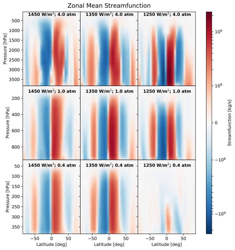


A more detailed look at some of the climates in our sample is given in Figure 5, Figure 6, Figure 7, and Figure 8. We find that our high-pressure climates are characterized by a slight poleward shift of the mid-latitude cloud belts, steeper potential temperature gradients at the tropopause, more-efficient poleward heat transport, and drier clouds. The lower cloud water specific humidity shown in Figure 8 is partly related to the greater stability against convection suggested by the potential temperature gradients in Figure 5—less-vigorous convection draws less water into the upper parts of the troposphere. We also find however that in the lower atmosphere, relative humidity is not particularly sensitive to surface pressure, suggesting that most of the overall decrease in cloud water specific humidity is not due to a proportional decrease in atmospheric water, but rather a consequence of the fact that the water saturation vapor pressure is a function only of temperature, so at higher pN2, a given parcel of air will reach saturation at a lower specific humidity. One of the snowball climates in our sample is shown in the bottom-right panel of each figure. Our snowball models have dry atmospheres and significantly weaker meridional circulation, consistent with the findings in Pierrehumbert 2005. Our models have increased temperatures at northern hemisphere mid-latitudes and therefore North-South asymmetries in streamfunction, cloud field, and atmospheric water content. This is due to land areas without snow and therefore lower albedo, as discussed in Paradise et al. 2019b.
3.2 Additional Experiments
| Experiment | Warming Trends | Cooling Trends |
|---|---|---|
| No Rayleigh Scattering | Yes | No |
| No Advection | Yes | Yes |
| No Sea-Ice Feedback | Yes | Yes |
| No Clouds | Yes | Yes |
| No Ozone | Yes | Yes |
| No Oceans; Wet Soil | Yes | Yes |
| No Water Vapor | No | Yes |
| No Water Vapor; No Advection | No | Yes |
| No Water Vapor; No Rayleigh Scattering | No | Yes |
| No Advection; No Water Vapor; No Scattering | Yes | No |
| No Pressure Broadening | No | Yes |
| No Advection; No H2O; No Scattering; No Broadening | No | Yes |
| No Advection; No H2O; No Scattering; No CO2 | No | No |
To investigate the physical mechanisms underlying the trends observed in Figure 2, we conducted several experiments changing initial conditions, boundary conditions, or model physics, described in subsection 2.4. Their results, excluding the elevated CO2 and snowball experiments, are summarized in Table 2.
Without heat transport or Rayleigh scattering, the global average temperature increases monotonically with increasing pN2, until our model crashes. The effect of pressure broadening from CO2 on its own is small—no more than 5–10 K between 1 and 10 bars of pN2. If either cooling from increased Rayleigh scattering or increased heat transport is present, that alone is enough to counteract the warming from pressure broadening of CO2, resulting in net cooling in dry atmospheres—pressure broadening of H2O absorption and amplification from the water vapor positive feedback are necessary for pressure-broadening to be the dominant mechanism. In the absence of water vapor, heat transport, scattering, or pressure broadening, a slight cooling trend remains—approximately 0.5 K over 1–10 bars. This cooling trend disappears when CO2 is removed as well, suggesting that the vertical distribution of CO2 in taller atmospheres is very slightly more efficient at cooling the surface.
To explore whether the warming by pressure broadening is primarily caused by broadening or CO2 absorption lines or H2O absorption, we re-ran the 1350 W/m2 slice of the parameter space in Figure 2 with 10 mbar of CO2 instead of 360 bar. The results are shown in Figure 9. While the higher-CO2 climates are significantly warmer, as expected, they demonstrate nearly identical sensitivity to increased pN2 as those with Earth-like pCO2. This suggests that absorption by water may be far more important for determining the climate’s sensitivity. This is consistent with our finding that availability of water vapor, not CO2, is necessary for an overall warming trend with increased pN2, and is consistent with Komacek and Abbot 2019 finding the same nonlinear response that we find, despite omitting CO2 from their models.
We examined the response of both temperate and snowball climates to differences in pN2, as shown in Figure 10. The temperate models display the strong, nonlinear response shown in Figure 2, with increased heating through pressure broadening amplified by abundant atmospheric water vapor, and eventual cooling by Rayleigh scattering. On the other hand, the snowball models appear much less sensitive to pN2, varying by only 4 K over 10 bars, despite the inclusion of the water vapor greenhouse effect.
3.3 Synchronous Rotators
We find that our tidally-locked models reproduce the major qualitative climate features observed in other simulations of tidally-locked planets, as shown in Figure 11. For temperate tidally-locked planets with Earth-like surface pressures, we find a nearly-circular area of above-freezing temperatures on the dayside, and nearly-uniform cold temperatures across much of the nightside (Pierrehumbert 2011), with a slight eastward offset of the substellar hot spot. The global temperature contrast increases as instellation decreases, as found by Haqq-Misra et al. 2018. Near the surface, air flows across the dayside toward the substellar point, where it rises, and then diverges in the upper troposphere, forming an eastward equatorial jet, guided by two strong high-latitude gyres on the nightside (Pierrehumbert 2011; Edson et al. 2011). The dayside upwelling region is humid, and thus has extensive cloud cover (Edson et al. 2011; Yang et al. 2013). We have not examined the sensitivity of these climate features to high or low pN2, and leave that investigation to a future study.
The minimum, mean, and maximum temperatures of our tidally-locked models, along with the global temperature contrast, are shown in Figure 12. The day-side sea ice fraction is shown in Figure 4. In this case we choose to show day-side sea ice instead of global sea ice because ice on the night-side does not reflect any light, and therefore the effect of varying background gas pressure on night-side ice is purely a consequence of ambient temperature, as opposed to ice on the day-side, where an ice albedo feedback exists in our models due to the solar-like input spectrum, and which may be affected by the Rayleigh scattering from elevated pN2. There appears to be some amount of complex structure in night-side temperatures in our high-instellation, high-pressure models, but due to few constraints on night-side climate in these regimes, we cannot rule out a numerical origin and recommend further study. On these planets, the climate is very sensitive to the efficiency with which heat can be advected from the dayside to the night side (Checlair et al. 2017; Haqq-Misra et al. 2018). As pN2 increases, heat transport efficiency increases, resulting in significant dayside cooling. Combined with increased Rayleigh scattering, warming by pressure broadening only dominates at low pN2 where heat transport and scattering are weak, and at high instellations where there is high potential for surface evaporation, resulting in very strong amplification through the water vapor greenhouse. In contrast to the Earth-like models in Figure 2, the surface pressure at which dayside surface temperatures are maximized has a strong dependence on surface pressure, moving to significantly lower pressures as instellation decreases, as shown in Figure 12. Here we are using changes in maximum temperature as the metric for the impact on the climate, in contrast to the average surface temperature, which we used in subsection 3.1. This is because the geometry of tidally-locked climates and the importance of horizontal heat transport on these planets means that changes in the global average surface temperature may not be particularly indicative of trends in the dayside climate. We find that just as with global sea ice extent on the Earth-like rotators, the transition from an ice-free dayside to a fully-frozen day-side on synchronous rotators is sharper at higher surface pressures. In general, we find that the increased importance of heat transport on tidally-locked planets results in increasing pN2 causing cooling in more of the parameter space than on fast-rotating Earth-like planets at the same pressures and instellations.
4 Discussion
4.1 Mechanisms of Action on the Climate
We find that three model components are responsible for the climate’s response to different background gas pressures. As was shown and briefly discussed in subsection 3.2, the primary contribution to cooling at higher pN2 in our experiments was the reduction in net shortwave heating due to increased reflection by Rayleigh scattering. Our results and those of Komacek and Abbot 2019 suggest that in some cases, Rayleigh scattering could be sufficient to force planets into a snowball state, similar to the maximum greenhouse phenomenon, where scattering by CO2 overcomes its greenhouse forcing (Kasting 1991; Kopparapu et al. 2013). Poleward heat transport does contribute to cooling on planets with Earth-like rotation, but to a lesser extent—its impact on global average temperatures is only apparent when the other major heating and cooling mechanisms are removed. We found that the warming trend in Figure 2 could only be reversed by eliminating the water vapor greenhouse effect, either by removing water vapor entirely or by removing pressure broadening. The effect of pressure broadening of H2O is much larger than the effect of broadening CO2 absorption in our models. This is because pressure broadening in PlaSim is an idealized multiplicative factor applied to broadband gas absorptivity, and water is both much more absorptive than CO2 and much more abundant in our models, so the magnitude of amplification for water is much larger than for CO2. A very small amount of cooling from increased pN2 remains when pressure broadening, heat transport, and evaporation have all been removed. When CO2 is also removed, the climate becomes completely insensitive to changes in pN2.
The amount of warming we find from the inclusion of water vapor is likely to have quantitative differences from what would be found in a more-sophisticated GCM, as the amount and altitude of stratospheric warming by ozone is prescribed in PlaSim. While we checked the effect of removing ozone entirely, we did not explore the impact that choosing different amounts of ozone would have. A more realistic treatment of ozone in atmospheres with varying amounts of background gas might result in different amounts of stratospheric warming, and therefore changes in the efficiency of the tropopause water trap. Similarly, as pressure-broadening in PlaSim is idealized, a more-sophisticated GCM may find different forcings from pressure-broadening of water vapor and CO2.
The relationship between these different mechanisms is very apparent when considering the difference between temperate Earth-like planets and snowball planets. In contrast to temperate planets, snowball planets demonstrate very low sensitivity to pN2. This low sensitivity is the result of cold temperatures and sea ice imposing limits on evaporation rates, thus limiting the strength of the water vapor positive feedback. The snowball models also appear less sensitive to cooling by Rayleigh scattering because the planet’s overall albedo is already very high, due to the highly-reflective surface. An increase in atmospheric albedo can therefore do little to raise the overall albedo, resulting in much smaller changes to the planet’s energy budget, as shown in Figure 13. In other words, the additional scattered light on a snowball planet is mostly light that would have been reflected anyway, as opposed to a temperate planet or a dry desert planet with a dark surface where that light would have been mostly absorbed. The importance of surface albedo in determining the climate’s sensitivity to pN2 suggests that any planet with a dark surface, i.e. planets without extensive ice or snow cover, will undergo strong cooling from increased Rayleigh scattering at high pN2. Land planets which are not completely dry, such as those in Abe et al. 2011, would exhibit strong cooling from Rayleigh scattering even at snowball-like temperatures, so long as the available water vapor did not produce extensive snow cover.
These results suggest that the effects of changing pN2 can be largely segregated into three different regimes:
- 1.
High pN2: Rayleigh scattering dominates, and adding pN2 cools the climate.
- 2.
Wet Surface: A large surface water reservoir permits strong evaporation at low pN2. The water vapor greenhouse effect dominates due to pressure broadening, and adding pN2 warms the climate.
- 3.
Dry Surface: Atmospheric water vapor is limited by low evaporation. Rayleigh scattering and heat transport are the dominant effects, and increasing pN2 cools the climate, even at low pN2.
Therefore on planets orbiting Sun-like stars with a limited water vapor greenhouse, either due to evaporation limited by sea ice or an overall lack of surface water, increasing pN2 results in colder climates, while the opposite effect is found on planets with large surface water inventories and enough radiative forcing to drive large amounts of evaporation. At sufficiently high pN2, other details of the climate matter less, as Rayleigh scattering is strong enough to cause cooling regardless of the planet’s water inventory. We do not expect a more-realistic layer-by-layer treatment of Rayleigh scattering in PlaSim to change this conclusion, as scattering in a high-pN2 atmosphere would simply occur above where water absorption would occur.
4.2 Impact of pN2 on Observables
Our findings in section 3 suggest that Earth-like climates are highly-sensitive to the amount of background gases present in the atmosphere. However, in the case of triple-bonded diatomic molecules like N2, the absence of prominent absorption lines in the visible or infrared (Lofthus and Krupenie 1977) makes it difficult to quantify the abundance of background gases on terrestrial planets with transit spectroscopy (Benneke and Seager 2012). Even if the Rayleigh scattering slope as a function of wavelength could be observed in transit spectroscopy, the presence of a cloud deck could limit efforts to constrain the total thickness of an atmosphere (Kaltenegger et al. 2007; Benneke and Seager 2012; Barstow et al. 2016). Observations using reflected light can more-easily probe deeper into the atmosphere (Snellen et al. 2015, e.g.), so we investigated the possibility that pN2 might have observable signatures in reflected light.
Our aim here is not to solve the inverse problem in a way that would permit robust and unique retrieval of background gas mass for real exoplanets, but instead to explore how different background gas pressures would affect observables. We therefore limit our analysis to spectra of the models shown in Figure 2, and do not systematically vary cloud fraction, land fraction, photochemistry, or any of the myriad other factors that might confound atmospheric retrievals. The B–V colors of our models are shown in Figure 14. Increasing pN2 results in stronger reflectance at short wavelengths compared to longer wavelengths, resulting in bluer planets. Very strong reflectance by surface ice seems to partially counteract this, potentially because with a reflective surface, red light that is scattered less efficiently than blue light is nonetheless reflected back to space, such that the overall color is relatively unchanged. Conversely, if the surface is dark, as is the case with open ocean, blue light will be scattered back to space while red light will be absorbed at the surface. Because ice is much more reflective than land or ocean, snowball planets therefore appear less blue at moderate background gas partial pressures. Once pN2 is sufficiently high, however, the atmosphere becomes optically-thick to Rayleigh scattering, surface information is obscured, and both temperate and snowball planets appear similarly blue. This applies not only to N2, but to any background gas that causes Rayleigh scattering. For background gases with significant absorption lines such as O2 or CO2, photometric color is probably not the easiest way to constrain atmospheric mass. For gases such as N2 that are otherwise difficult to detect, this finding that thick atmospheres tend to be blue in the absence of color-altering phenomena like photochemical hazes may aid inference efforts.
4.3 Caveats
While we believe our results are robust due to qualitative agreement with ExoCAM (Komacek and Abbot 2019) and the 1D models used in Goldblatt et al. 2009 and Keles et al. 2018, as well as consistency across a diversity of climates, there are nonetheless a number of model caveats that make any quantitative predictions of specific climates suspect. Perhaps most importantly, PlaSim’s implementation of Rayleigh scattering assumes that all scattering happens at the atmosphere’s bottom layer, which is not physically realistic. The impact on the climate’s energy budget for Earth-like surface pressures and lower is negligible, as the atmosphere’s exponential density profile means most scattering does indeed happen in the lower layers of the atmosphere, below cloud tops, and absorption by the surface is the primary way visible light enters the climate’s energy budget in the regimes we have modeled(Pierrehumbert 2010). However, at higher surface pressures, scattering at higher levels of the atmosphere may become important. In models more realistic than PlaSim, atmospheric absorption of visible and near-infrared light by water vapor and oxygen also contributes to the climate’s energy budget (Fujii et al. 2017; Kopparapu et al. 2017; Way et al. 2017, e.g.), and scattering in the middle and upper atmosphere may affect that.
In addition to shortcomings in the scattering parameterization, PlaSim’s ozone abundance is prescribed as a normal distribution peaked at 20 km above the surface. This may be appropriate for Earth’s atmosphere, but likely incorrect for planets with different N2 and O2 partial pressures. As the height of peak ozone absorption affects stratospheric heating and therefore the height and temperature of the tropopause (Wordsworth and Pierrehumbert 2014), and as this will affect the strength of water-trapping at the tropopause (Zahnle and Buick 2016), more work is needed to understand how ozone and photochemistry are affected by different background gas partial pressures, and how their climate feedbacks therefore respond.
While our results show a sharp transition from ice-free states to fully-frozen states at high pressures, we have refrained from examining how the snowball bistability is affected by elevated pN2. This is because the mechanisms by which the climate enters and exits snowball are key to understanding the width of the bistability. An exploration of the changes in the bistability at higher surface pressures should therefore incorporate more-sophisticated GCMs that include key model physics, such as ocean circulation and sea ice drift, and include detailed analysis of how glaciation and deglaciation occur at high pressures. We therefore leave the question of the snowball bistability to future work.
As mentioned in subsection 4.2, we have also not considered the role that photochemistry, hazes, aerosols, and differences in cloud formation efficiency might play in thick N2 atmospheres. In addition to affecting observables, these factors would likely also affect the climate’s energy budget (Arney et al. 2017; Chen et al. 2018; Chen et al. 2019). Most of these factors are not feasible to study fully with PlaSim, and so would require further work with a more sophisticated model.
We have assumed a solar-like input spectrum in all of our models. One of the major mechanisms by which N2 affects the climate is Rayleigh scattering, which is most efficient at short wavelengths due to a dependence, where is wavelength(Rybicki and Lightman 2004). Earth-like planets around lower-mass stars would instead receive most of their light at red and infrared wavelengths, meaning Rayleigh scattering’s contribution to the climate’s energy budget would be lessened considerably. We have shown this in Figure 15, in which we calculated how the broadband scattering optical depth for a gas like N2 changes for planets orbiting stars throughout the main sequence. In these climates, we can likely expect cooling through heat transport and warming through pressure broadening to be the dominant ways that N2 affects the climate, as the reduced importance of Rayleigh scattering at high pN2 will reduce the impact of pN2 on shortwave heating. Some work has already been done to explore the impact of changing pN2 on tidally-locked planets orbiting red stars (Turbet et al. 2018), but this has yet to be fully-explored across the habitable zone in a systematic manner, which we leave to future work.
Finally, we did not compute spectra for our tidally-locked models, as almost all real tidally-locked planets will orbit cooler stars with redder spectra (Pierrehumbert 2011). As discussed in the previous paragraph, Rayleigh scattering will be much less important on those planets, so our tidally-locked planets are not representative of the climates likely to be found on real tidally-locked exoplanets. Computing reflected spectra for our tidally-locked models would therefore yield little useful information about the impact of background gas partial pressure on observables. Further work that models tidally-locked planets with appropriately-red input spectra, as in Turbet et al. 2016; Turbet et al. 2018; Fauchez et al. 2019, and Yang et al. 2019, is needed. In particular, future work should aim to produce systematic surveys of the tidally-locked parameter space across the habitable zone.
5 Conclusion
We have used a large ensemble of GCMs in which pN2 was varied for a range of instellations and initial conditions, for both Earth-like and tidally-locked rotation, and for both aquaplanet and modern Earth land distributions. We found that the climate’s response to pN2 is strong and nonlinear, with increasing pN2 leading to warming in some regimes, and cooling in others. We performed a number of experiments to isolate the mechanisms responsible, and conclude that at low and moderate surface pressures on planets with large surface water reservoirs for evaporation, pressure broadening of the CO2 and H2O absorption lines leads to significant heating. At high surface pressures and in dry climates, Rayleigh scattering dominates over pressure broadening, leading to cooling. On planets with very efficient cooling through horizontal heat transport, such as tidally-locked planets, increased heat transport at high surface pressures further leads to cooling, reducing the potential of pressure broadening to cause net warming. Our results are consistent with those reported in Komacek and Abbot 2019, Goldblatt et al. 2009, and Keles et al. 2018, and demonstrate the relationship between the various competing mechanisms explored in the literature thus far (Nakajima et al. 1992; Goldblatt et al. 2009; Kaspi and Showman 2015; Zahnle and Buick 2016, e.g.). Finally, we showed that while pN2 may be difficult to quantify with transit spectroscopy, high pN2 will result in planets appearing ‘bluer’ in reflected light, which may eventually be detectable with broadband reflected light photometry through either direct imaging using coronagraphy (Stark et al. 2015, e.g.), or through secondary eclipse spectroscopy using differential photometric measurements (Belu et al. 2010, e.g.).
The history of Earth’s pN2 is poorly-constrained (Olson et al. 2018), and we have little to no constraints on likely N2 partial pressures on terrestrial exoplanets, particularly those with formation histories and stellar environments different from our own. Even within our own solar system, pN2 varies between terrestrial planets with atmospheres—Venus has over 3 bars of N2 in its atmosphere (Oyama et al. 1980). Our results show however that pN2 is a crucial ingredient in assessing a planet’s climate and habitability. We have determined that pN2 will have an impact on observables accessible through direct imaging and secondary eclipse spectroscopy, but more work is needed to understand its role and evolution on planets with both Earth-like and non-Earth-like geophysical and geochemical properties. Furthermore, while increased pN2 has been proposed as a possible resolution to the ‘faint young Sun paradox’ (Johnson and Goldblatt 2017), in our sample increased pN2 alone (i.e., without increasing CO2 from its present level) is not able to sufficiently warm an Earth-like planet at Archaean Earth instellation. We have not however fully-explored the range of possible Archaean atmospheres, which likely hosted 10-2500 times the present level of CO2 (Catling and Zahnle 2020). Similarly, studies of the potential habitability and climate of specific exoplanets will need to consider a broad and systematic range of atmospheric compositions and masses, as some recent studies using GCMs (Turbet et al. 2016; Del Genio et al. 2018; Turbet et al. 2018, e.g.) have begun to do.
6 Acknowledgments
AP is supported by the Department of Astronomy & Astrophysics at the University of Toronto, BLF is supported by the Department of Physics at the University of Toronto, KM is supported by the Natural Sciences and Engineering Research Council of Canada, and CL is supported by the Department of Physics at the University of Toronto. Computing resources were provided by the Canadian Institute for Theoretical Astrophysics at the University of Toronto. The authors would like to thank Dorian Abbot for suggestions of existing literature on the role of pN2 in the climate, and the attendees of the Comparative Climatology of Terrestrial Planets III conference in Houston, Texas in August 2018 for an enlightening and thought-provoking discussion about the difficulties in reconstructing the early Earth’s pN2 history and evolution. The authors would also like to thank Colin Goldblatt and the anonymous referees for their helpful comments and suggestions, particularly with regards to the model validation in Figure 1. The modified version of PlaSim used in this study is available on AP’s github (Paradise et al. 2019a).
We would furthermore like to acknowledge that our work was performed on land traditionally inhabited by the Wendat, the Anishnaabeg, Haudenosaunee, Métis, and the Mississaugas of the Credit First Nation. We also note that this work required supercomputing infrastructure, whose availability was only possible through the mining of precious metals from ecologically-sensitive areas around the world that are traditionally inhabited by Indigenous peoples.
7 Model Data Availability
The model outputs from this paper are being made available online through Dataverse (Paradise et al. 2020).
References
- Abbot et al. (2018)
Abbot, D. S., Bloch-Johnson, J., Checlair, J., Farahat, N. X., Graham, R. J.,
Plotkin, D., Popovic, P., Spaulding-Astudillo, F., feb 2018. Decrease in
Hysteresis of Planetary Climate for Planets with Long Solar Days. The
Astrophysical Journal 854 (1), 3.
URL http://arxiv.org/abs/1801.10551http://dx.doi.org/10.3847/1538-4357/aaa70fhttp://stacks.iop.org/0004-637X/854/i=1/a=3?key=crossref.e0325e68e507678dff38fffd59736583 - Abe et al. (2011) Abe, Y., Abe-Ouchi, A., Sleep, N. H., Zahnle, K. J., 2011. Habitable zone limits for dry planets. Astrobiology 11 (5), 443–460.
- Arney et al. (2017)
Arney, G. N., Meadows, V. S., Domagal-Goldman, S. D., Deming, D., Robinson,
T. D., Tovar, G., Wolf, E. T., Schwieterman, E., 2017. Pale Orange Dots: The
Impact of Organic Haze on the Habitability and Detectability of Earthlike
Exoplanets. The Astrophysical Journal 836 (1), 49.
URL http://arxiv.org/abs/1702.02994 - Barstow et al. (2016) Barstow, J. K., Aigrain, S., Irwin, P. G., Kendrew, S., Fletcher, L. N., 2016. Telling twins apart: Exo-Earths and Venuses with transit spectroscopy. Monthly Notices of the Royal Astronomical Society 458 (3), 2657–2666.
- Belu et al. (2010) Belu, A. R., Selsis, F., Morales, J. C., Ribas, I., Cossou, C., Rauer, H., 2010. Primary and secondary eclipse spectroscopy with JWST: Exploring the exoplanet parameter space. Astronomy and Astrophysics 525 (4), 1–15.
- Benneke and Seager (2012)
Benneke, B., Seager, S., 2012. Atmospheric Retrieval for Super-Earths:
Uniquely Constraining the Atmospheric Composition With Transmission
Spectroscopy. The Astrophysical Journal 753 (2), 100.
URL http://arxiv.org/abs/1203.4018{%}5Cnhttp://dx.doi.org/10.1088/0004-637X/753/2/100 - Berner (2004) Berner, R. A., 2004. The Phanerozoic Carbon Cycle: CO2 and O2. Oxford University Press, New York.
- Bin et al. (2018)
Bin, J., Tian, F., Liu, L., 2018. New inner boundaries of the habitable zones
around M dwarfs. Earth and Planetary Science Letters 492, 121–129.
URL https://doi.org/10.1016/j.epsl.2018.04.003 - Binney and Merrifield (1998) Binney, J., Merrifield, M., 1998. Galactic Astronomy. Princeton University Press.
- Boschi et al. (2013) Boschi, R., Lucarini, V., Pascale, S., Nov 2013. Bistability of the climate around the habitable zone: A thermodynamic investigation. Icarus 226 (2), 1724–1742.
- Boutle et al. (2017)
Boutle, I. A., Mayne, N. J., Drummond, B., Manners, J., Goyal, J., Hugo
Lambert, F., Acreman, D. M., Earnshaw, P. D., may 2017. Exploring the
climate of Proxima B with the Met Office Unified Model. Astronomy &
Astrophysics 601 (2016), A120.
URL http://arxiv.org/abs/1702.08463http://dx.doi.org/10.1051/0004-6361/201630020http://www.aanda.org/10.1051/0004-6361/201630020 - Budyko (1969) Budyko, M. I., oct 1969. The effect of solar radiation variations on the climate of the Earth. Tellus 21 (5), 611–619.
- Catling and Zahnle (2020)
Catling, D. C., Zahnle, K. J., feb 2020. The Archean atmosphere. Science
Advances 6 (9), eaax1420.
URL https://advances.sciencemag.org/lookup/doi/10.1126/sciadv.aax1420 - Charnay et al. (2013) Charnay, B., Forget, F., Wordsworth, R., Leconte, J., Millour, E., Codron, F., Spiga, A., Sep 2013. Exploring the faint young Sun problem and the possible climates of the Archean Earth with a 3-D GCM. Journal of Geophysical Research (Atmospheres) 118 (18), 10,414–10,431.
- Checlair et al. (2017)
Checlair, J., Menou, K., Abbot, D. S., aug 2017. No Snowball on Habitable
Tidally Locked Planets. The Astrophysical Journal 845 (2), 132.
URL http://arxiv.org/abs/1705.08904http://dx.doi.org/10.3847/1538-4357/aa80e1http://stacks.iop.org/0004-637X/845/i=2/a=132?key=crossref.0179b453ba8de0d24a234f4256873009 - Chemke and Kaspi (2017)
Chemke, R., Kaspi, Y., 2017. Dynamics of Massive Atmospheres. The
Astrophysical Journal 845 (1), 1.
URL http://dx.doi.org/10.3847/1538-4357/aa7742 - Chemke et al. (2016) Chemke, R., Kaspi, Y., Halevy, I., Nov 2016. The thermodynamic effect of atmospheric mass on early Earth’s temperature. Geophysical Research Letters 43 (21), 11,414–11,422.
- Chen et al. (2018)
Chen, H., Wolf, E. T., Kopparapu, R., Domagal-Goldman, S., Horton, D. E., nov
2018. Biosignature Anisotropy Modeled on Temperate Tidally Locked M-dwarf
Planets. The Astrophysical Journal 868 (1), L6.
URL http://stacks.iop.org/2041-8205/868/i=1/a=L6?key=crossref.1bae0bdea0b2bbfa97039895721d00b8 - Chen et al. (2019)
Chen, H., Wolf, E. T., Zhan, Z., Horton, D. E., 2019. Habitability and
Spectroscopic Observability of Warm M-dwarf Exoplanets Evaluated with a 3D
Chemistry-Climate Model.
URL http://arxiv.org/abs/1907.10048 - Del Genio et al. (2018)
Del Genio, A. D., Way, M. J., Amundsen, D. S., Aleinov, I., Kelley, M.,
Kiang, N. Y., Clune, T. L., sep 2018. Habitable Climate Scenarios for
Proxima Centauri b with a Dynamic Ocean. Astrobiology 19 (2), ast.2017.1760.
URL https://www.liebertpub.com/doi/10.1089/ast.2017.1760 - D’Errico et al. (2018) D’Errico, M., Faranda, D., Yiou, P., Nardini, C., Dec 2018. Detection and attribution of Southern European cold spells via a statistical Mechanics Approach. In: AGU Fall Meeting Abstracts. Vol. 2018. pp. GC21E–1138.
- Edson et al. (2011)
Edson, A., Lee, S., Bannon, P., Kasting, J. F., Pollard, D., 2011. Atmospheric
circulations of terrestrial planets orbiting low-mass stars. Icarus 212 (1),
1–13.
URL http://dx.doi.org/10.1016/j.icarus.2010.11.023 - Fauchez et al. (2019) Fauchez, T., Turbet, M., Wolf, E. T., Boutle, I., Way, M. J., Del Genio, A. D., Mayne, N. J., Tsigaridis, K., Kopparapu, R. K., Yang, J., Forget, F., Mandell, A., Domagal Goldman, S. D., 2019. TRAPPIST-1 Habitable Atmosphere Intercomparison (THAI). Motivations and protocol. Geoscientific Model Development Discussions (August), 1–15.
- Fraedrich et al. (2005) Fraedrich, K., Jansen, H., Kirk, E., Luksch, U., Lunkeit, F., 2005. The Planet Simulator: Towards a user friendly model. Meteorologische Zeitschrift 14 (3), 299–304.
- Fujii et al. (2017)
Fujii, Y., Del Genio, A. D., Amundsen, D. S., oct 2017. NIR-driven Moist
Upper Atmospheres of Synchronously Rotating Temperate Terrestrial
Exoplanets. The Astrophysical Journal 848 (2), 100.
URL http://dx.doi.org/10.3847/1538-4357/aa8955http://stacks.iop.org/0004-637X/848/i=2/a=100?key=crossref.d049c184d313285db725725be5971d36 - Goldblatt et al. (2009) Goldblatt, C., Claire, M. W., Lenton, T. M., Matthews, A. J., Watson, A. J., Zahnle, K. J., Dec 2009. Nitrogen-enhanced greenhouse warming on early Earth. Nature Geoscience 2 (12), 891–896.
- Goldblatt et al. (2013) Goldblatt, C., Robinson, T. D., Zahnle, K. J., Crisp, D., 2013. Low simulated radiation limit for runaway greenhouse climates. Nature Geoscience 6 (8), 661–667.
- Gómez-Leal et al. (2018)
Gómez-Leal, I., Kaltenegger, L., Lucarini, V., Lunkeit, F., dec 2018.
Climate Sensitivity to Carbon Dioxide and the Moist Greenhouse Threshold of
Earth-like Planets under an Increasing Solar Forcing. The Astrophysical
Journal 869 (2), 129.
URL https://linkinghub.elsevier.com/retrieve/pii/S0019103517307820http://arxiv.org/abs/1901.02901http://dx.doi.org/10.3847/1538-4357/aaea5fhttps://iopscience.iop.org/article/10.3847/1538-4357/aaea5f - Haqq-Misra et al. (2018)
Haqq-Misra, J., Wolf, E. T., Joshi, M., Zhang, X., Kopparapu, R. K., jan 2018.
Demarcating Circulation Regimes of Synchronously Rotating Terrestrial
Planets within the Habitable Zone. The Astrophysical Journal 852 (2), 67.
URL http://arxiv.org/abs/1710.00435http://stacks.iop.org/0004-637X/852/i=2/a=67?key=crossref.31470b49165c69127c4c420f6aa490fe - Holden et al. (2016) Holden, P. B., Edwards, N. R., Fraedrich, K., Kirk, E., Lunkeit, F., Zhu, X., Sep 2016. PLASIM-GENIE v1.0: a new intermediate complexity AOGCM. Geoscientific Model Development 9, 3347–3361.
- Ingle and Crouch (1988) Ingle, J. J., Crouch, S., 1 1988. Spectrochemical analysis.
- Johnson and Goldblatt (2015) Johnson, B., Goldblatt, C., 2015. The nitrogen budget of Earth. Earth-Science Reviews 148, 150–173.
- Johnson and Goldblatt (2017)
Johnson, B., Goldblatt, C., sep 2017. A secular increase in continental crust
nitrogen during the Precambrian. Geochemical Perspectives Letters, 24–28.
URL http://arxiv.org/abs/1709.02412{%}0Ahttp://dx.doi.org/10.7185/geochemlet.1731http://www.geochemicalperspectivesletters.org/article1731 - Kaltenegger et al. (2007)
Kaltenegger, L., Traub, W. A., Jucks, K. W., mar 2007. Spectral Evolution of
an Earth-like Planet. The Astrophysical Journal 658 (1), 598–616.
URL https://doi.org/10.1086{%}2F510996http://stacks.iop.org/0004-637X/658/i=1/a=598 - Kaspi and Showman (2015)
Kaspi, Y., Showman, A. P., may 2015. ATMOSPHERIC DYNAMICS OF TERRESTRIAL
EXOPLANETS OVER A WIDE RANGE OF ORBITAL AND ATMOSPHERIC PARAMETERS. The
Astrophysical Journal 804 (1), 60.
URL http://arxiv.org/abs/1407.6349http://dx.doi.org/10.1088/0004-637X/804/1/60http://stacks.iop.org/0004-637X/804/i=1/a=60?key=crossref.0ab2282fe18e8ff907c5692589c99aeehttps://iopscience.iop.org/article/10.1088/0004-637X/804/1/60 - Kasting (1991)
Kasting, J. F., nov 1991. CO2 condensation and the climate of early Mars.
Icarus 94 (1), 1–13.
URL https://linkinghub.elsevier.com/retrieve/pii/001910359190137I - Kasting et al. (1993)
Kasting, J. F., Whitmire, D. P., Reynolds, R. T., 1993. Habitable Zones around
Main Sequence Stars.
URL http://linkinghub.elsevier.com/retrieve/pii/S0019103583710109 - Keles et al. (2018) Keles, E., Grenfell, J. L., Godolt, M., Stracke, B., Rauer, H., 2018. The effect of varying atmospheric pressure upon habitability and biosignatures of earth-like planets. Astrobiology 18 (2), 116–132.
- Kiehl et al. (1996) Kiehl, J., Hack, J., Bonan, G., Boville, B., Briegleb, B., Williamson, D., Rasch, P., 1996. Description of the NCAR Community Climate Model (CCM3). Tech. Rep. September.
- Koll and Cronin (2019)
Koll, D. D. B., Cronin, T. W., 2019. Hot Hydrogen Climates near the inner edge
of the Habitable Zone. The Astrophysical Journal 881 (2), 120.
URL http://arxiv.org/abs/1907.13169 - Komacek and Abbot (2019)
Komacek, T. D., Abbot, D. S., feb 2019. The Atmospheric Circulation and
Climate of Terrestrial Planets Orbiting Sun-like and M Dwarf Stars over a
Broad Range of Planetary Parameters. The Astrophysical Journal 871 (2), 245.
URL http://arxiv.org/abs/1901.00567http://dx.doi.org/10.3847/1538-4357/aafb33http://stacks.iop.org/0004-637X/871/i=2/a=245?key=crossref.058e5787c42138cbe5ae3fc87aae806d - Kopparapu et al. (2013)
Kopparapu, R. K., Ramirez, R., Kasting, J. F., Eymet, V., Robinson, T. D.,
Mahadevan, S., Terrien, R. C., Domagal-Goldman, S., Meadows, V., Deshpande,
R., 2013. Habitable Zones Around Main-Sequence Stars: New Estimates. The
Astrophysical Journal 765 (2), 131.
URL http://stacks.iop.org/0004-637X/765/i=2/a=131?key=crossref.2f4b541791428841b8a64638c66c631c - Kopparapu et al. (2014) Kopparapu, R. K., Ramirez, R. M., Schottelkotte, J., Kasting, J. F., Domagal-Goldman, S., Eymet, V., 2014. Habitable zones around main-sequence stars: Dependence on planetary mass. Astrophysical Journal Letters 787 (2), 1–14.
- Kopparapu et al. (2017)
Kopparapu, R. K., Wolf, E. T., Arney, G., Batalha, N. E., Haqq-Misra, J.,
Grimm, S. L., Heng, K., aug 2017. Habitable Moist Atmospheres on Terrestrial
Planets near the Inner Edge of the Habitable Zone around M Dwarfs. The
Astrophysical Journal 845 (1), 5.
URL http://arxiv.org/abs/1705.10362{%}0Ahttp://dx.doi.org/10.3847/1538-4357/aa7cf9http://stacks.iop.org/0004-637X/845/i=1/a=5?key=crossref.4a1c0801f894be11ccd75326674fb990 - Kuo (1965)
Kuo, H. L., jan 1965. On Formation and Intensification of Tropical Cyclones
Through Latent Heat Release by Cumulus Convection. Journal of the
Atmospheric Sciences 22 (1), 40–63.
URL http://journals.ametsoc.org/doi/abs/10.1175/1520-0469{%}281965{%}29022{%}3C0040{%}3AOFAIOT{%}3E2.0.CO{%}3B2 - Kuo (1974)
Kuo, H. L., jul 1974. Further Studies of the Parameterization of the Influence
of Cumulus Convection on Large-Scale Flow. Journal of the Atmospheric
Sciences 31 (5), 1232–1240.
URL http://journals.ametsoc.org/doi/abs/10.1175/1520-0469{%}281974{%}29031{%}3C1232{%}3AFSOTPO{%}3E2.0.CO{%}3B2 - Lacis and Hansen (1974)
Lacis, A. A., Hansen, J., 1974. A parameterization for the absorption of solar
radiation in the earth’s atmosphere. Journal of the Atmospheric Sciences
31 (1), 118–133.
URL https://doi.org/10.1175/1520-0469(1974)031<0118:APFTAO>2.0.CO;2 - Leconte et al. (2013) Leconte, J., Forget, F., Charnay, B., Wordsworth, R., Pottier, A., Dec. 2013. Increased insolation threshold for runaway greenhouse processes on Earth-like planets. Nature 504 (7479), 268–271.
- Li et al. (2009) Li, K.-F., Pahlevan, K., Kirschvink, J. L., Yung, Y. L., Jun 2009. Atmospheric pressure as a natural climate regulator for a terrestrial planet with a biosphere. Proceedings of the National Academy of Science 106 (24), 9576–9579.
- Lofthus and Krupenie (1977)
Lofthus, A., Krupenie, P. H., jan 1977. The spectrum of molecular nitrogen.
Journal of Physical and Chemical Reference Data 6 (1), 113–307.
URL http://aip.scitation.org/doi/10.1063/1.555546 - Manabe and Wetherald (1975)
Manabe, S., Wetherald, R. T., 1975. The effects of doubling the co2
concentration on the climate of a general circulation model. Journal of the
Atmospheric Sciences 32 (1), 3–15.
URL https://doi.org/10.1175/1520-0469(1975)032<0003:TEODTC>2.0.CO;2 - Menou (2013)
Menou, K., aug 2013. WATER-TRAPPED WORLDS. The Astrophysical Journal 774 (1),
51.
URL http://arxiv.org/abs/1304.6472{%}0Ahttp://dx.doi.org/10.1088/0004-637X/774/1/51http://stacks.iop.org/0004-637X/774/i=1/a=51?key=crossref.6afe4455e5ecb8ca63c9c618e09c6ec7 - Nakajima et al. (1992)
Nakajima, S., Hayashi, Y.-Y., Abe, Y., dec 1992. A Study on the “Runaway
Greenhouse Effect” with a One-Dimensional Radiative–Convective
Equilibrium Model. Journal of the Atmospheric Sciences 49 (23), 2256–2266.
URL http://journals.ametsoc.org/doi/abs/10.1175/1520-0469{%}281992{%}29049{%}3C2256{%}3AASOTGE{%}3E2.0.CO{%}3B2 - Nakayama et al. (2019) Nakayama, A., kodama, T., Ikoma, M., Abe, Y., Jul 2019. Runaway climate cooling of ocean planets in the habitable zone: a consequence of seafloor weathering enhanced by melting of high-pressure ice. arXiv e-prints, arXiv:1907.00827.
- Nowajewski et al. (2018) Nowajewski, P., Rojas, M., Rojo, P., Kimeswenger, S., May 2018. Atmospheric dynamics and habitability range in Earth-like aquaplanets obliquity simulations. Icarus 305, 84–90.
- Olson et al. (2018)
Olson, S. L., Schwieterman, E. W., Reinhard, C. T., Lyons, T. W., mar 2018.
Earth: Atmospheric Evolution of a Habitable Planet. In: Handbook of
Exoplanets. Springer International Publishing, Cham, pp. 1–37.
URL http://link.springer.com/10.1007/978-3-319-30648-3{_}189-1http://arxiv.org/abs/1803.05967http://dx.doi.org/10.1007/978-3-319-30648-3{_}189-1 - Oyama et al. (1980)
Oyama, V. I., Carle, G. C., Woeller, F., Pollack, J. B., Reynolds, R. T.,
Craig, R. A., 1980. Pioneer venus gas chromatography of the lower atmosphere
of venus. Journal of Geophysical Research: Space Physics 85 (A13),
7891–7902.
URL https://agupubs.onlinelibrary.wiley.com/doi/abs/10.1029/JA085iA13p07891 - Paradise et al. (2019a)
Paradise, A., Borth, H., Lunkeit, F., Kirk, E., Mar. 2019a.
alphaparrot/gplasim: Radiative flexibility.
URL https://doi.org/10.5281/zenodo.2602241 - Paradise et al. (2020)
Paradise, A., Fan, B. L., Menou, K., Lee, C., 2020. PlaSim Models: “Climate
Diversity in the Solar-Like Habitable Zone due to Varying Background Gas
Pressure”.
URL https://doi.org/10.5683/SP2/LOFVCV - Paradise and Menou (2017)
Paradise, A., Menou, K., 2017. GCM Simulations of Unstable Climates in the
Habitable Zone. The Astrophysical Journal 848 (1), 33.
URL http://dx.doi.org/10.3847/1538-4357/aa8b1c - Paradise et al. (2019b)
Paradise, A., Menou, K., Valencia, D., Lee, C., aug 2019b.
Habitable Snowballs: Temperate Land Conditions, Liquid Water, and
Implications for CO 2 Weathering. Journal of Geophysical Research: Planets
124 (8), 2087–2100.
URL http://arxiv.org/abs/1803.00511https://onlinelibrary.wiley.com/doi/abs/10.1029/2019JE005917 - Pierrehumbert (2005) Pierrehumbert, R., 2005. Climate dynamics of a hard snowball earth. Journal of Geophysical Research 110 (D1), 1–22.
- Pierrehumbert (2010) Pierrehumbert, R., 2010. Principles of Planetary Climate. Cambridge University Press, New York.
- Pierrehumbert (2011)
Pierrehumbert, R. T., jan 2011. A PALETTE OF CLIMATES FOR GLIESE 581g. The
Astrophysical Journal 726 (1), L8.
URL http://stacks.iop.org/2041-8205/726/i=1/a=L8?key=crossref.cec1f483122516f25084273c0e08d529 - Ramirez (2018)
Ramirez, R., jul 2018. A More Comprehensive Habitable Zone for Finding Life on
Other Planets. Geosciences 8 (8), 280.
URL http://arxiv.org/abs/1807.09504{%}0Ahttp://www.mdpi.com/2076-3263/8/8/280http://www.mdpi.com/2076-3263/8/8/280 - Ricchiazzi et al. (1998)
Ricchiazzi, P., Yang, S., Gautier, C., Sowle, D., oct 1998. SBDART: A Research
and Teaching Software Tool for Plane-Parallel Radiative Transfer in the
Earth’s Atmosphere. Bulletin of the American Meteorological Society 79 (10),
2101–2114.
URL http://journals.ametsoc.org/doi/abs/10.1175/1520-0477{%}281998{%}29079{%}3C2101{%}3ASARATS{%}3E2.0.CO{%}3B2 - Rybicki and Lightman (2004) Rybicki, G. B., Lightman, A. P., 2004. Radiative Processes in Astrophysics, 2nd Edition. Wiley-VCH, Weinheim.
- Sagan and Mullen (1972)
Sagan, C., Mullen, G., jul 1972. Earth and Mars: Evolution of Atmospheres and
Surface Temperatures. Science 177 (4043), 52–56.
URL https://science.sciencemag.org/content/177/4043/52http://www.sciencemag.org/cgi/doi/10.1126/science.177.4043.52 - Sasamori (1968)
Sasamori, T., 1968. The radiative cooling calculation for application to
general circulation experiments. Journal of Applied Meteorology 7 (5),
721–729.
URL https://doi.org/10.1175/1520-0450(1968)007<0721:TRCCFA>2.0.CO;2 - Sellers (1969)
Sellers, W. D., 1969. A global climatic model based on the energy balance of
the earth-atmosphere system. Journal of Applied Meteorology 8 (3), 392–400.
URL https://doi.org/10.1175/1520-0450(1969)008<0392:AGCMBO>2.0.CO;2 - Shields et al. (2016)
Shields, A. L., Barnes, R., Agol, E., Charnay, B., Bitz, C., Meadows, V. S.,
jun 2016. The Effect of Orbital Configuration on the Possible Climates and
Habitability of Kepler-62f. Astrobiology 16 (6), 443–464.
URL http://arxiv.org/abs/1603.01272http://dx.doi.org/10.1089/ast.2015.1353http://online.liebertpub.com/doi/10.1089/ast.2015.1353 - Slingo and Slingo (1991)
Slingo, A., Slingo, J. M., 1991. Response of the National Center for
Atmospheric Research community climate model to improvements in the
representation of clouds. Journal of Geophysical Research 96 (D8), 15341.
URL http://doi.wiley.com/10.1029/91JD00930 - Snellen et al. (2015)
Snellen, I. A. G., de Kok, R., Birkby, J. L., Brandl, B., Brogi, M., Keller,
C. U., Kenworthy, M., Schwarz, H., Stuik, R., 2015. Combining
high-dispersion spectroscopy with high contrast imaging: Probing rocky
planets around our nearest neighbors. Astronomy & Astrophysics 576 (3),
A59.
URL http://arxiv.org/abs/1503.01136{%}5Cnhttp://adsabs.harvard.edu/abs/2015A{&}A...576A..59S - Som et al. (2016) Som, S. M., Buick, R., Hagadorn, J. W., Blake, T. S., Perreault, J. M., Harnmeijer, J. P., Catling, D. C., 2016. Earth’s air pressure 2.7 billion years ago constrained to less than half of modern levels. Nature Geoscience 9 (6), 448–451.
- Stark et al. (2015)
Stark, C. C., Roberge, A., Mandell, A., Clampin, M., Domagal-Goldman, S. D.,
McElwain, M. W., Stapelfeldt, K. R., jul 2015. LOWER LIMITS ON APERTURE SIZE
FOR AN EXOEARTH DETECTING CORONAGRAPHIC MISSION. The Astrophysical Journal
808 (2), 149.
URL http://dx.doi.org/10.1088/0004-637X/808/2/149https://iopscience.iop.org/article/10.1088/0004-637X/808/2/149 - Stephens (1978)
Stephens, G. L., nov 1978. Radiation Profiles in Extended Water Clouds. II:
Parameterization Schemes. Journal of the Atmospheric Sciences 35 (11),
2123–2132.
URL http://journals.ametsoc.org/doi/abs/10.1175/1520-0469{%}281978{%}29035{%}3C2123{%}3ARPIEWC{%}3E2.0.CO{%}3B2 - Stephens (1984)
Stephens, G. L., apr 1984. The Parameterization of Radiation for Numerical
Weather Prediction and Climate Models. Monthly Weather Review 112 (4),
826–867.
URL http://journals.ametsoc.org/doi/abs/10.1175/1520-0493{%}281984{%}29112{%}3C0826{%}3ATPORFN{%}3E2.0.CO{%}3B2 - Stephens et al. (1984)
Stephens, G. L., Ackerman, S., Smith, E. A., feb 1984. A Shortwave
Parameterization Revised to Improve Cloud Absorption. Journal of the
Atmospheric Sciences 41 (4), 687–690.
URL http://journals.ametsoc.org/doi/abs/10.1175/1520-0469{%}281984{%}29041{%}3C0687{%}3AASPRTI{%}3E2.0.CO{%}3B2 - Strong and Plass (1950) Strong, J., Plass, G. N., Nov. 1950. The Effect of Pressure Broadening of Spectral Lines on Atmospheric Temperature. The Astrophysical Journal 112, 365.
- Stüeken et al. (2016)
Stüeken, E. E., Kipp, M. A., Koehler, M. C., Schwieterman, E. W.,
Johnson, B., Buick, R., 2016. Modeling pN2 through Geological Time:
Implications for Planetary Climates and Atmospheric Biosignatures.
Astrobiology 16 (12), 33.
URL http://arxiv.org/abs/1612.02865 - Turbet et al. (2018)
Turbet, M., Bolmont, E., Leconte, J., Forget, F., Selsis, F., Tobie, G.,
Caldas, A., Naar, J., Gillon, M., apr 2018. Modeling climate diversity,
tidal dynamics and the fate of volatiles on TRAPPIST-1 planets. Astronomy
& Astrophysics 612, A86.
URL https://www.aanda.org/10.1051/0004-6361/201731620 - Turbet et al. (2016)
Turbet, M., Leconte, J., Selsis, F., Bolmont, E., Forget, F., Ribas, I.,
Raymond, S. N., Anglada-Escudé, G., dec 2016. The habitability of
Proxima Centauri b. Astronomy & Astrophysics 596, A112.
URL http://arxiv.org/abs/1608.06919http://www.aanda.org/10.1051/0004-6361/201629577 - Valencia et al. (2018) Valencia, D., Tan, V. Y. Y., Zajac, Z., Apr 2018. Habitability from Tidally Induced Tectonics. The Astrophysical Journal 857 (2), 106.
- Vladilo et al. (2013)
Vladilo, G., Murante, G., Silva, L., Provenzale, A., Ferri, G., Ragazzini, G.,
feb 2013. The habitable zone of Earth-like planets with different levels of
atmospheric pressure. The Astrophysical Journal 767 (1), 65.
URL http://arxiv.org/abs/1302.4566{%}0Ahttp://dx.doi.org/10.1088/0004-637X/767/1/65http://stacks.iop.org/0004-637X/767/i=1/a=65?key=crossref.9d747f20949ec9f33cc162f00e5da089http://arxiv.org/abs/1302.4566http://dx.doi.org/10.1088/0004-637X/767/1/65 - Walker et al. (1981) Walker, J., Hays, P., Kasting, J., 1981. A negative feedback mechanism for the long-term stabilization of earth’s surface temperature. Journal of Geophysical Research 86 (C10), 9776–9782.
- Way et al. (2017)
Way, M. J., Aleinov, I., Amundsen, D. S., Chandler, M. A., Clune, T. L., Genio,
A. D. D., Fujii, Y., Kelley, M., Kiang, N. Y., Sohl, L., Tsigaridis, K., jul
2017. Resolving Orbital and Climate Keys of Earth and Extraterrestrial
Environments with Dynamics (ROCKE-3D) 1.0: A General Circulation Model for
Simulating the Climates of Rocky Planets. The Astrophysical Journal
Supplement Series 231 (1), 12.
URL http://stacks.iop.org/0067-0049/231/i=1/a=12?key=crossref.2440b27e9f0a7debc0b27c7bc18e2247 - Williams and Kasting (1997)
Williams, D. M., Kasting, J. F., sep 1997. Habitable Planets with High
Obliquities. Icarus 129 (1), 254–267.
URL http://www.sciencedirect.com/science/article/pii/S0019103597957596https://linkinghub.elsevier.com/retrieve/pii/S0019103597957596 - Wolf and Toon (2014)
Wolf, E., Toon, O., 2014. Controls on the archean climate system investigated
with a global climate model. Astrobiology 14 (3), 241–253, pMID: 24621308.
URL https://doi.org/10.1089/ast.2013.1112 - Wolf (2017)
Wolf, E. T., apr 2017. Assessing the Habitability of the TRAPPIST-1 System
Using a 3D Climate Model. The Astrophysical Journal 839 (1), L1.
URL http://arxiv.org/abs/1703.05815http://dx.doi.org/10.3847/2041-8213/aa693ahttp://stacks.iop.org/2041-8205/839/i=1/a=L1?key=crossref.1f8babc828488896844eea0df54a6712 - Wordsworth (2016)
Wordsworth, R., aug 2016. Atmospheric nitrogen evolution on Earth and Venus.
Earth and Planetary Science Letters 447, 103–111.
URL https://linkinghub.elsevier.com/retrieve/pii/S0012821X16301583 - Wordsworth and Pierrehumbert (2014) Wordsworth, R., Pierrehumbert, R., 2014. Abiotic oxygen-dominated atmospheres on terrestrial habitable zone planets. Astrophysical Journal Letters 785 (2), 2–5.
- Yang et al. (2014)
Yang, J., Boué, G., Fabrycky, D. C., Abbot, D. S., 2014. Strong
Dependence of the Inner Edge of the Habitable Zone on Planetary Rotation
Rate. The Astrophysical Journal 787 (1), L2.
URL http://stacks.iop.org/2041-8205/787/i=1/a=L2?key=crossref.4f04854c3caf03a7945b2d3eae682ffc - Yang et al. (2013)
Yang, J., Cowan, N. B., Abbot, D. S., 2013. Stabilizing Cloud Feedback
Dramatically Expands the Habitable Zone of Tidally Locked Planets. The
Astrophysical Journal 771 (2), L45.
URL http://stacks.iop.org/2041-8205/771/i=2/a=L45?key=crossref.dad84a2284f357b75182157e7808b044 - Yang et al. (2019)
Yang, J., Leconte, J., Wolf, E. T., Merlis, T., Koll, D. D. B., Forget, F.,
Abbot, D. S., 2019. Simulations of Water Vapor and Clouds on Rapidly
Rotating and Tidally Locked Planets: A 3D Model Intercomparison. The
Astrophysical Journal 875 (1), 46.
URL http://dx.doi.org/10.3847/1538-4357/ab09f1 - Zahnle and Buick (2016)
Zahnle, K., Buick, R., may 2016. Ancient air caught by shooting stars. Nature
533 (7602), 184–186.
URL http://www.nature.com/articles/533184a