The Role of A-priori Information in Networks of Rational Agents This work is partially supported by a grant from the Blavatnik Cyber Security Council, the Blavatnik Family Computer Science Research Fund and the KIPP Foundation.

The connection between distributed computing and game theory stemmed from the problem of secret sharing [32]. Further works continued the research on secret sharing and multiparty computation when both Byzantine and rational agents are present [2, 18, 21, 22, 23, 29].

Another line of research presented the BAR model (Byzantine, acquiescent and rational) [8, 31, 37], while a related line of research discusses converting solutions with a mediator to cheap talk [2, 3, 12, 13, 19, 26, 30, 33, 35, 36].

Abraham, Dolev, and Halpern [4] were the first to present protocols for networks of rational agents, specifically protocols for Leader Election. In [5] the authors continue this line of research by providing basic building blocks for game theoretic distributed algorithms, namely a wake-up and knowledge sharing equilibrium building blocks. Algorithms for consensus, renaming, and leader election are presented using these building blocks. Consensus was researched further by Halpern and Vilacça [24], who showed that there is no ex-post Nash equilibrium, and a Nash equilibrium that tolerates $f$ failures under some minimal assumptions on the failure pattern. Yifrach and Mansour [38] studied fair Leader Election protocols, giving an almost tight resilience analysis. Bank, Sulamy, and Waserman [11] examined the case where the $id$ space is limited, calculating the minimal threshold for equilibrium.

Coloring and Knowledge Sharing have been studied extensively in a distributed setting [9, 10, 17, 25, 27, 28, 34]. An algorithm for Knowledge Sharing with rational agents was presented in [5], while Coloring with rational agents has not been studied previously, to the best of our knowledge.

Informally, a distributed algorithm is an equilibrium if no agent at no point in the execution can do better by unilaterally deviating from the algorithm. When considering a deviation, an agent assumes all other agents follow the algorithm, i.e., it is the only agent deviating.

Formally, let $o_{a}$ be the output of agent $a$, let $\Theta$ be the set of all possible output vectors, and denote the output vector $O=(o_{1},\dots,o_{n})\in\Theta$, where $O[a]=o_{a}$. Let $\Theta_{L}$ be the set of legal output vectors, in which the protocol terminates successfully, and let $\Theta_{E}$ be the set of erroneous output vectors, such that $\Theta=\Theta_{L}\cup\Theta_{E}$ and $\Theta_{L}\cap\Theta_{E}=\varnothing$.

Each agent $a$ has a utility function $u_{a}:\Theta\rightarrow\mathbb{N}$. The higher the value assigned by $u_{a}$ to an output vector, the better this vector is for $a$. As in previous works [4, 5, 38], the utility function is required to satisfy the Solution Preference property which guarantees that an agent never has an incentive to fail the algorithm. Otherwise, they would simply be Byzantine faults. An agent fails the algorithm only when it detects that another agent had deviated.

We differentiate the legal output vectors, which ensure the output is valid and not erroneous, from the correct output vectors, which are output vectors that are a result of a correct execution of the algorithm, i.e., without any deviation. Solution Preference guarantees agents never prefer an erroneous output. However, they may prefer a legal but incorrect output.

The Solution Preference property introduces the threat agents face when deviating: Agents know that if another agent catches them cheating, it outputs $\bot$ and the algorithm fails. In other words, the output is erroneous, i.e., in $\Theta_{E}$.

For simplicity, we assume agents only have preferences over their own output, i.e., for any $O_{1},O_{2}\in\Theta_{L}$ in which $O_{1}[a]=O_{2}[a]$, $u_{a}(O_{1})=u_{a}(O_{2})$. Additionally, each agent $a$ has a single preferred output value $p_{a}$, and we normalize the utility function values, such that²² 2 This is the weakest assumption since it still leaves a cheating agent with the highest incentive to deviate, while still satisfying Solution Preference. A utility assigning a lower value for failure than $o_{a}\neq p_{a}$ would deter a cheating agent from deviating. :

These assumptions are for convenience only and can easily be removed. Our results hold for any utility function that satisfies Solution Preference.

We can also consider the expected utility from following a strategy. Let $S_{a}$ denote a series of steps for agent $a$ beginning at round $r$ until the end of the protocol, i.e., a list of actions $a$ performs every round from $r$ and on. These may specify different reactions to situations during the course of the protocol. Then we can consider all possible outputs where $a$ acts according to $S_{a}$ and other agents act according to the protocol, and denote the expected utility over all these outputs as $\mathbb{E}_{S_{a},r}[u_{a}]$.

An agent will deviate whenever the deviating step has a strictly higher expected utility than the expected utility of the next step of the algorithm, even if that deviating step also increases the risk of an erroneous output.

Let $\Lambda$ be an algorithm. If by deviating from $\Lambda$ and taking step $s$, the expected utility of $a$ is higher, we say that agent $a$ has an incentive to deviate (i.e., cheat). For example, at round $r$ algorithm $\Lambda$ may dictate that $a$ flips a fair binary coin and sends the result to all of its neighbors. Any other action by $a$ is considered a deviation: whether the message was not sent to all neighbors, sent later than it should have, or whether the coin toss was not fair, e.g., $a$ only sends $0$ instead of a random value. If no agent can unilaterally increase its expected utility by deviating from $\Lambda$, we say that the protocol is an equilibrium. Equilibrium is defined over a single deviating agent, i.e., there are no coalitions of agents.

Distributed Equilibrium is a sort of truthful equilibrium: a protocol where if agents assume all other agents follow the protocol truthfully, their best action is to truthfully follow the protocol as well.

It is important to emphasize that for any non-trivial distributed algorithm, the outcome cannot be calculated using only private data, without communication. For rational agents, no agent can calculate the output privately at the beginning of the algorithm, since if it could calculate the output and know that its resulting utility will be $0$, it would surely lie over its initial information to avoid losing, preventing equilibrium. If it knows its resulting utility is $1$, it has no incentive to cheat. But then there exists an instance of the same problem where the agents has a different preference over the output, making that protocol not an equilibrium. Formally, for any agent $a$ and any step $s$ of the agent that does not necessarily result in algorithm failure, it must hold that: $\mathbb{E}_{s,0}[u_{a}]\notin\{0,1\}$ (a value of $0$ means an agent will surely not get its preference, and $1$ means it is guaranteed to get its preference).

In Section 4 and Section 5 agents are in a Bayesian environment where they do not know $n$, the size of the network, but instead know a prior $\sigma$ over $\mathbb{N}$ from which $n$ originates. The support of $\sigma$ is:

The Knowledge Sharing problem (adapted from [5]) is defined as follows:

1. 1.

   Each agent $a$ has a private input $i_{a}$, in addition to its $id$, and a function $q$, where $q$ is identical at all agents. Agents know the possible output space of $q$ before the algorithm begins.

2. 2.

   A Knowledge Sharing protocol terminates legally if all agents output the same value, i.e., $\forall{a,b}:o_{a}=o_{b}\neq\bot$. Thus the set $\Theta_{L}$ is defined as: $O\in\Theta_{L}\iff\forall{a,b}:O(a)=O(b)\neq\bot$.

3. 3.

   A Knowledge Sharing protocol terminates correctly (as described in Section 2.1) if each agent outputs the value $q(I)$ over the input values $I=\{i_{1},\dots,i_{n}\}$ of all other agents⁴⁴ 4 Notice that any output is legal as long as it is the output of all agents, but only a single output value is considered correct for a given input vector..

4. 4.

   The function $q$ satisfies the Full Knowledge property:

   Definition 2.8 (Full Knowledge Property).

   A function $q$ fulfills the full knowledge property if, for each agent that does not know the input values of all other agents, any output in the range of $q$ is equally possible. Formally, for any $1\leq j\leq m$, fix $(x_{1},\dots,x_{j-1},x_{j+1},\dots,x_{m})$ and denote $z_{y}=|\{x_{j}|q(x_{1},\dots,x_{j},\dots,x_{m})=y\}|$. A function $q$ fulfills the full knowledge property if, for any possible output $y$ in the range of $q$, $z_{y}$ is the same⁵⁵ 5 The definition assumes input values are drawn uniformly, otherwise the definition of $z_{y}$ can be expanded to the sum of probabilities over every input value for $x_{j}$..

We differentiate two variants of Knowledge Sharing:

• •

  $k$-Knowledge Sharing - where $|range(q)|=k$ and $k$ is known to all agents at the beginning of the algorithm. For example, in $2$-Knowledge Sharing the output space is $\{0,1\}$ and all agents know the possible outputs of the protocol are from $\{0,1\}$. If every agent’s input is a random bit, a $2$-Knowledge Sharing protocol performs a shared coin flip.

• •

  Knowledge Sharing - A protocol for Knowledge Sharing is a protocol that solves $k$-Knowledge Sharing for any possible $k$. In the same manner, a protocol is an equilibrium if for any possible $k\in\mathbb{N}$, no agent has an incentive to cheat.

We assume that each agent $a$ prefers a certain output value $p_{a}$.

In the Coloring problem [17, 27], $\Theta_{L}$ is any $O$ such that $\forall{a}:o_{a}\neq\bot$ and $\forall{(a,b)\in E}:o_{a}\neq o_{b}$. We assume that every agent $a$ prefers a specific color $p_{a}$.

Let $a$ be a malicious agent with $\delta$ outgoing edges. A possible deviation for $a$ is to simulate imaginary agents $a_{1}$, $a_{2}$ and to answer over some of its edges as $a_{1}$, and over the others as $a_{2}$, as illustrated in Figure 1. From this point on $a$ acts as if it is 2 agents. We assume that the id space is much larger than $n$, allowing us to disregard the probability that the fake id collides with an existing id, an issue dealt with in [11].

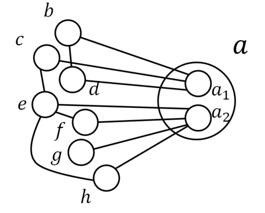
Regarding the output vector, notice that an agent that pretends to be more than one agent still outputs a single output at the end. The duplication causes agents to execute the algorithm as if it is executed on a graph $G^{\prime}$ (with the duplicated agents) instead of the original graph $G$; however, the output is considered legal if $O=(o_{a},o_{b},\dots)\in\Theta_{L}$ rather than if $(o_{a_{1}},o_{a_{2}},o_{b},\dots)\in\Theta_{L}$.

First we describe the Secret-Transmit($i_{a}$,$r$,$b$) building block in which agent $b$ learns the input $i_{a}$ of agent $a$ at round $r$, and no other agent in the ring learns any information about this input. To achieve this, agent $a$ selects a random number $R_{a}$, and let $X_{a}=R_{a}\oplus i_{a}$. It sends $R_{a}$ clockwise and $X_{a}$ counter-clockwise until each reaches the agent before $b$. At round $r-1$, these neighbors of $b$ simultaneously send $b$ the values $X_{a}$ and $R_{a}$, thus $b$ receives the information at round $r$.

We assume a global orientation around the ring. This assumption can easily be relaxed via Leader Election [5], which is an equilibrium in this application since the orientation has no effect on the output. The algorithm works as follows:

Here, agents are given exact a-priori knowledge of $n$.

We present Algorithm 2, the Witness Algorithm, that uses two subroutines to obtain a coloring: Draw and Prompt.

The Witness algorithm includes three colorings: The agents already have an $n$-coloring set by their $id$s. But agents can cheat by lying about their $id$s. So each agent selects a new unique number from $1$ to $n$, in a way that prevents it from cheating about the number. That is another $n$-coloring of the agents, but this coloring does not ensure that every agent $a$ with no neighbors that output $p_{a}$ will output $p_{a}$. Thus, an agent that can still output $p_{a}$ legally, i.e., none of its neighbors are numbered $p_{a}$, will output $p_{a}$ instead of its unique number, which may also cause an illegal coloring in case two neighbors with the same preferred color behave this way. Instead, this second $n$-coloring is used as the order by which agents choose their final color, resulting in a legal coloring in which agents have no incentive to cheat.

The algorithm begins by running Wake-Up [5] to learn the graph topology and the $id$s of all agents. Then, in order of $id$s, each agent $a$ draws a random number $S(a)$ with a neighboring ”witness” agent $w(a)$ as specified in Algorithm 3, and sends it to all of its neighbors. The number is drawn in the range $1,\dots,n$ and since agents draw numbers one by one, each agent knows the set of numbers already taken by its neighbors and uses it as the input $T$ for its call to Draw, ensuring no two neighbors draw the same number and resulting in a coloring of $G$. However, this coloring is not enough since any equilibrium must ensure an agent that can output its desired color will output it. In Draw, the agent cannot cheat in the random number generation process since it exchanges a random number simultaneously with its respective witness, and $w(a)$ is marked as a witness for future verification, ensuring $a$ will not lie about its drawn number. When done, each agent simultaneously verifies the numbers published by its neighbors using Algorithm 4, which enables it to receive each value through two disjoint paths: directly from the neighbor, and via the shortest simple path to the neighbor’s witness that does not include the neighbor. Then each agent, in order of the values drawn randomly, picks its preferred color if available, or the minimal available color otherwise, and sends its color to all of its neighbors.

Draw (Algorithm 3) is an equilibrium in which agent $a$ randomizes a number different from those of its neighbors and commits to it, and is depicted in Figure 5. For an arbitrary agent $a$ and a subset $T$ of numbers from $\{1,\dots,n\}$, Draw begins with $a$ sending its neighbor with minimum $id$ the string witness. The following round, $a$ and the agent that received the witness string exchange a random number from $1$ to $|X|$ at the same time, where $X=\{1\dots n\}\setminus T$. The sum of these two randomized numbers $\mod|X|$, denoted $q$, is calculated at $a$ and at its witness, and then $a$ notifies all its neighbors that its result from the Draw process is the $q$’th largest number in $X$, ensuring that when these neighbors use Draw, they do not include that number in their respective $X$. Draw takes a constant number of rounds to complete, denoted $|Draw|$ rounds. Prompt (Algorithm 4) is a query that ensures $a$ receives the correct drawn number from a neighbor.

The complexity of the Witness Algorithm is $O(|E|\cdot n)$.

The resulting message complexity is:

• •

  Wake Up is $O(|E|\cdot n)$

• •

  Drawing a random number is called $n$ times and uses a total of $O(|E|)$ messages in total to publish these values to neighbors

• •

  Verifying the value of a neighbor uses $O(diameter)$ messages and is called $O(|E|)$ times, for a total of $O(|E|\cdot diameter)$

• •

  Sending the output color takes an additional $O(|E|)$ messages

Since the diameter of the network is at most $n$ (line graph), we have a total of $O(|E|\cdot n)$.

In ring networks, we have shown Algorithm 1 is an equilibrium if no agent duplicates $d>n$. In other words, the only way an agent $a$ can increase its expected utility is by duplicating into at least $2$ more agents than the size of the remainder of the ring, i.e., $n^{\prime}$ is made of $n-1$ honest agents and at least $n+1$ duplicated cheater agents. It is easy to see that if a cheating agent had duplicated $d>n$ agents and was not detected (i.e., $d+n-1\leq\beta$), its utility is $1$ since it controls the output. Notice that Algorithm 1 begins with Wake-Up, so a duplicating agent must decide on its duplication scheme before any communication other than Wake-Up occurs.

We consider a specific duplication scheme for the cheating agent: Duplicating $d=\lfloor\frac{\beta}{2}\rfloor+1$. This cheating strategy maximizes a cheater’s expected utility by obtaining the optimal balance between $P_{D}$ and successfully duplicating $d>n$ (recall that $n$ is a random variable from the cheater’s perspective). Notice that duplicating $d>n$ is beneficial only when $\beta\geq 2\alpha$. If $\beta<2\alpha$, duplicating $d=\lfloor\frac{\beta}{2}\rfloor+1$ would either be detected and lead to $0$ utility, or in case $n=\alpha$, would result in $d=n$ and not increase the cheater’s utility. Any duplication other than $d=\lfloor\frac{\beta}{2}\rfloor+1$ would also result in $d\leq n$ (which does not improve the cheater’s expected utility) or in detection.

Let $a$ be an agent in the ring at round $0$ with prior $n\sim\sigma$. Let $D$ be a cheating strategy in which $a$ duplicates into $d=\lfloor\frac{\beta}{2}\rfloor+1$ agents, and if $a$ is not caught, it skews the protocol to output $p_{a}$. The expected utility by following strategy D is:

If for all agents this utility is at most $\mathbb{E}_{\Gamma}[u_{a}]=\frac{1}{k}$, the expected utility from following the protocol, then Algorithm 1 is an equilibrium. Setting the probability mass function F and $d=\lfloor\frac{\beta}{2}\rfloor+1$ yields the following requirement for Algorithm 1 to be an equilibrium:

For each prior and each Knowledge Sharing variant, if $\mathbb{E}_{D,0}[u_{a}]>\frac{1}{k}$ then there is an incentive to cheat by duplicating $d=\lfloor\frac{\beta}{2}\rfloor+1$, and then using an optimal cheating strategy that derives a utility of $1$. Table 2 shows the conditions on $[\alpha,\beta]$ for Algorithm 1 to be an equilibrium. Following the table are explanations of each entry.

1. 1.

   For uniform $\sigma$ and $k=2$, setting the probability mass function $F$ for the uniform distribution into Equation 2 yields:

   $$\frac{\lfloor\frac{\beta}{2}\rfloor-\alpha+1}{\beta-\alpha+1}+\frac{1}{2}\bigg(\frac{\lceil\frac{\beta}{2}\rceil-\lfloor\frac{\beta}{2}\rfloor}{\beta-\alpha+1}\bigg)\leq\frac{1}{2}$$

   $$\frac{\lfloor\frac{\beta}{2}\rfloor-\alpha+1}{\beta-\alpha+1}\leq\frac{1}{2}\bigg(\frac{\beta-\alpha+1-\lceil\frac{\beta}{2}\rceil+\lfloor\frac{\beta}{2}\rfloor}{\beta-\alpha+1}\bigg)$$

   $$\lfloor\frac{\beta}{2}\rfloor-\alpha+1\leq\frac{1}{2}\bigg(2\cdot\lceil\frac{\beta}{2}\rceil-\alpha+1\bigg)$$

   $$2\cdot\lfloor\frac{\beta}{2}\rfloor-2\alpha+2\leq 2\cdot\lfloor\frac{\beta}{2}\rfloor-\alpha+1$$

   $$\alpha\geq 1$$

   This inequality holds for any $\alpha,\beta$. Thus when $k=2$ and $\sigma$ is a uniform prior, Algorithm 1 is an equilibrium for any $\alpha,\beta$.

2. 2.

   When $\sigma$ is uniform and $k>2$, setting the probability mass function $F$ for the uniform distribution into Equation 2:

   $$\frac{\lfloor\frac{\beta}{2}\rfloor-\alpha+1}{\beta-\alpha+1}+\frac{1}{k}\bigg(\frac{\lceil\frac{\beta}{2}\rceil-\lfloor\frac{\beta}{2}\rfloor}{\beta-\alpha+1}\bigg)\leq\frac{1}{k}$$

   $$\frac{\lfloor\frac{\beta}{2}\rfloor-\alpha+1}{\beta-\alpha+1}\leq\frac{1}{k}\bigg(\frac{\beta-\alpha+1+\lfloor\frac{\beta}{2}\rfloor-\lceil\frac{\beta}{2}\rceil}{\beta-\alpha+1}\bigg)$$

   $$(\lfloor\frac{\beta}{2}\rfloor-\alpha+1)\leq\frac{1}{k}\big(\beta-\alpha+1+\lfloor\frac{\beta}{2}\rfloor-\lceil\frac{\beta}{2}\rceil\big)=\frac{1}{k}\big(2\cdot\lfloor\frac{\beta}{2}\rfloor-\alpha+1\big)$$

   $$k\leq\frac{2\cdot\lfloor\frac{\beta}{2}\rfloor-\alpha+1}{\lfloor\frac{\beta}{2}\rfloor-\alpha+1}=1+\frac{\lfloor\frac{\beta}{2}\rfloor}{\lfloor\frac{\beta}{2}\rfloor-\alpha+1}$$

   (3)

   We can then consider two cases for $\beta$:

   • •

     $\beta$ is even:

     $$k\leq 1+\frac{\beta}{\beta-2\alpha+2}$$

     $$\beta\leq\frac{(2\alpha-2)(k-1)}{k-2}$$

   • •

     $\beta$ is odd, then using the same derivation:

     $$k\leq\frac{\beta-1}{\beta-1-2\alpha+2}$$

     $$\beta\leq\frac{2\alpha(k-1)-k}{k-2}$$

   Notice that for any $k>2$, the even upper bound is lower, so Algorithm 1 is an equilibrium if and only if:

   $$\beta\leq\frac{(2\alpha-2)(k-1)}{k-2}$$

3. 3.

   We now want to know the bounds on $[\alpha,\beta]$ for which we have a general Knowledge Sharing protocol that is an equilibrium, namely, a Knowledge Sharing protocol that is an equilibrium for any $k$. Notice that we assume agents always know $k$ beforehand, but we require that the same equilibrium should apply to any $k$. We can see that the demand for an equilibrium for constant $k$, namely:

   $$\beta\leq\frac{(2\alpha-2)(k-1)}{k-2}$$

   Actually shows that as a function of $k$, the upper bound for an equilibrium converges to $\beta\leq 2\alpha-1$. In other words, for any uniform $\sigma$ with $\beta\geq 2\alpha$, there exists a $k$ large enough so that the protocol is not an equilibrium, i.e., there exists an agent with an incentive to cheat. As stated above, if $\beta\leq 2\alpha-1$, Algorithm 1 is an equilibrium, because no agent can duplicate $d>n$ without surely being detected.

4. 4.

   When $\sigma$ is geometric, consider Equation 2. Notice that if the inequality holds, Algorithm 1 is an equilibrium. If $\beta$ is even, the left hand side of the inequality is smaller. Assume that $\beta$ is even, we get that Equation 2 yields that Algorithm 1 is an equilibrium when :

   $$F(\frac{\beta}{2})\leq\frac{1}{k}$$

   By definition of $F$ for a geometric prior, $\text{Pr}[n=\alpha]>\frac{1}{2}$. In other words, for any $\beta\geq 2\alpha$ and any $k\geq 2$, $F(\frac{\beta}{2})>\frac{1}{2}\geq\frac{1}{k}$. So a cheating agent $a$ has an incentive to deviate for any $k$ and any $\beta\geq 2\alpha$. The same holds for the case where $\beta$ is odd.

In this section we show that for any ring and any prior on $n$ with finite support $\sigma\subseteq[\alpha,\beta]$ in which Algorithm 1 is an equilibrium for $2$-Knowledge Sharing, there is an equilibrium for Coloring. We describe Algorithm 5, which uses a shared coin toss subroutine. Using Algorithm 1, we set each agent’s input be a random bit and define the output function $q(\vec{I})=\sum_{i\in I}i\mod 2$. This shared coin toss subroutine is an equilibrium as a subroutine if agents’ utilities are either a direct result of the output of the coin flip, or completely independent of it.

References

- [1] I. Abraham, L. Alvisi, and J. Y. Halpern. Distributed computing meets game theory: Combining insights from two fields. SIGACT News, 42(2):69–76, June 2011.
- [2] I. Abraham, D. Dolev, R. Gonen, and J. Y. Halpern. Distributed computing meets game theory: robust mechanisms for rational secret sharing and multiparty computation. In PODC, pages 53–62, 2006.
- [3] I. Abraham, D. Dolev, and J. Y. Halpern. Lower bounds on implementing robust and resilient mediators. In TCC, pages 302–319, 2008.
- [4] I. Abraham, D. Dolev, and J. Y. Halpern. Distributed protocols for leader election: A game-theoretic perspective. In DISC, pages 61–75, 2013.
- [5] Y. Afek, Y. Ginzberg, S. Landau Feibish, and M. Sulamy. Distributed computing building blocks for rational agents. In Proceedings of the 2014 ACM Symposium on Principles of Distributed Computing, PODC ’14.
- [6] Y. Afek, S. Rafaeli, and M. Sulamy. Cheating by Duplication: Equilibrium Requires Global Knowledge. ArXiv e-prints, Nov. 2017.
- [7] Y. Afek, S. Rafaeli, and M. Sulamy. The Role of A-priori Information in Networks of Rational Agents. In U. Schmid and J. Widder, editors, 32nd International Symposium on Distributed Computing (DISC 2018), volume 121 of Leibniz International Proceedings in Informatics (LIPIcs), pages 5:1–5:18, Dagstuhl, Germany, 2018. Schloss Dagstuhl–Leibniz-Zentrum fuer Informatik.
- [8] A. S. Aiyer, L. Alvisi, A. Clement, M. Dahlin, J.-P. Martin, and C. Porth. Bar fault tolerance for cooperative services. In SOSP, pages 45–58, 2005.
- [9] H. Attiya and J. Welch. Distributed Computing: Fundamentals, Simulations and Advanced Topics. John Wiley & Sons, 2004.
- [10] B. Awerbuch, M. Luby, A. V. Goldberg, and S. A. Plotkin. Network decomposition and locality in distributed computation. In Proceedings of the 30th Annual Symposium on Foundations of Computer Science, SFCS ’89, pages 364–369, Washington, DC, USA, 1989. IEEE Computer Society.
- [11] D. Bank, M. Sulamy, and E. Waserman. Reaching Distributed Equilibrium with Limited ID Space. ArXiv e-prints, Apr. 2018.
- [12] I. Bárány. Fair distribution protocols or how the players replace fortune. Math. Oper. Res., 17(2):327–340, May 1992.
- [13] E. Ben-Porath. Cheap talk in games with incomplete information. J. Economic Theory, 108(1):45–71, 2003.
- [14] R. Bhattacharjee and A. Goel. Avoiding ballot stuffing in ebay-like reputation systems. In Proceedings of the 2005 ACM SIGCOMM Workshop on Economics of Peer-to-peer Systems, P2PECON ’05, pages 133–137, New York, NY, USA, 2005. ACM.
- [15] M. Bianchini, M. Gori, and F. Scarselli. Inside pagerank. ACM Trans. Internet Technol., 5(1):92–128, Feb. 2005.
- [16] A. Cheng and E. Friedman. Sybilproof reputation mechanisms. In Proceedings of the 2005 ACM SIGCOMM Workshop on Economics of Peer-to-peer Systems, P2PECON ’05, pages 128–132, New York, NY, USA, 2005. ACM.
- [17] R. Cole and U. Vishkin. Deterministic coin tossing with applications to optimal parallel list ranking. Inf. Control, 70(1):32–53, July 1986.
- [18] V. Dani, M. Movahedi, Y. Rodriguez, and J. Saia. Scalable rational secret sharing. In PODC, pages 187–196, 2011.
- [19] Y. Dodis, S. Halevi, and T. Rabin. A cryptographic solution to a game theoretic problem. In CRYPTO, pages 112–130, 2000.
- [20] J. R. Douceur. The sybil attack. In Revised Papers from the First International Workshop on Peer-to-Peer Systems, IPTPS ’01, pages 251–260, London, UK, UK, 2002. Springer-Verlag.
- [21] G. Fuchsbauer, J. Katz, and D. Naccache. Efficient rational secret sharing in standard communication networks. In TCC, pages 419–436, 2010.
- [22] S. D. Gordon and J. Katz. Rational secret sharing, revisited. In SCN, pages 229–241, 2006.
- [23] A. Groce, J. Katz, A. Thiruvengadam, and V. Zikas. Byzantine agreement with a rational adversary. In ICALP (2), pages 561–572, 2012.
- [24] J. Y. Halpern and X. Vilaça. Rational consensus: Extended abstract. In Proceedings of the 2016 ACM Symposium on Principles of Distributed Computing, PODC ’16, pages 137–146, New York, NY, USA, 2016. ACM.
- [25] F. Kuhn and R. Wattenhofer. On the complexity of distributed graph coloring. In Proceedings of the Twenty-fifth Annual ACM Symposium on Principles of Distributed Computing, PODC ’06, pages 7–15, New York, NY, USA, 2006. ACM.
- [26] M. Lepinski, S. Micali, C. Peikert, and A. Shelat. Completely fair sfe and coalition-safe cheap talk. In PODC, pages 1–10, 2004.
- [27] N. Linial. Legal coloring of graphs. Combinatorica, 6(1):49–54, 1986.
- [28] N. Linial. Distributive graph algorithms global solutions from local data. In Proceedings of the 28th Annual Symposium on Foundations of Computer Science, SFCS ’87, pages 331–335, Washington, DC, USA, 1987. IEEE Computer Society.
- [29] A. Lysyanskaya and N. Triandopoulos. Rationality and adversarial behavior in multi-party computation. In CRYPTO, pages 180–197, 2006.
- [30] R. McGrew, R. Porter, and Y. Shoham. Towards a general theory of non-cooperative computation. In TARK, pages 59–71, 2003.
- [31] T. Moscibroda, S. Schmid, and R. Wattenhofer. When selfish meets evil: byzantine players in a virus inoculation game. In PODC, pages 35–44, 2006.
- [32] A. Shamir. How to share a secret. Commun. ACM, 22(11):612–613, 1979.
- [33] Y. Shoham and M. Tennenholtz. Non-cooperative computation: Boolean functions with correctness and exclusivity. Theoretical Computer Science, 343(1–2):97 – 113, 2005.
- [34] M. Szegedy and S. Vishwanathan. Locality based graph coloring. In Proceedings of the Twenty-fifth Annual ACM Symposium on Theory of Computing, STOC ’93, pages 201–207, New York, NY, USA, 1993. ACM.
- [35] A. Urbano and J. E. Vila. Computational complexity and communication: Coordination in two-player games. Econometrica, 70(5):1893–1927, September 2002.
- [36] A. Urbano and J. E. Vila. Computationally restricted unmediated talk under incomplete information. Economic theory, 2004.
- [37] E. L. Wong, I. Levy, L. Alvisi, A. Clement, and M. Dahlin. Regret freedom isn’t free. In OPODIS, pages 80–95, 2011.
- [38] A. Yifrach and Y. Mansour. Fair Leader Election for Rational Agents. PODC ’18.