Gravitational Wave Signals from Multiple Hidden Sectors
Abstract
We explore the possibility of detecting gravitational waves generated by first-order phase transitions in multiple dark sectors. naturalness is taken as a sample model that features multiple additional sectors, many of which undergo phase transitions that produce gravitational waves. We examine the cosmological history of this framework and determine the gravitational wave profiles generated. These profiles are checked against projections of next-generation gravitational wave experiments, demonstrating that multiple hidden sectors can indeed produce unique gravitational wave signatures that will be probed by these future experiments.
I Introduction
The recent experimental detection of gravitational waves Abbott et al. 2016 gives humanity a new way to observe the universe. Future experiments Danzmann 1994; Seto et al. 2001; Crowder and Cornish 2005a; Crowder and Cornish 2005b; Harry et al. 2006; Janssen et al. 2015; Audley et al. 2017; Amaro-Seoane et al. 2017; et al 2017; Isoyama et al. 2018 will greatly expand the frequency range observable. Thus far, experiments have only observed recent events such as black hole mergers, but phase transitions in the early universe can leave an imprint as a stochastic gravitational wave background Witten 1984; Hogan 1983; Hogan 1986; Turner and Wilczek 1990; Caprini et al. 2016; Mazumdar and White 2019. Thus, searches for this background of gravitational waves can give direct information of the history of the universe before big bang nucleosynthesis. Because gravity is universal, gravitational waves can allow us to probe hidden sectors that couple very weakly, or not at all, to the Standard Model as long they are reheated after inflation. This was first explored in Schwaller 2015, and there has been significant work on this idea since Jaeckel et al. 2016; Addazi 2017; Hardy 2017; Dienes et al. 2017; Tsumura et al. 2017; Acharya et al. 2017; Bernal et al. 2017; Aoki et al. 2017; Heikinheimo et al. 2018; Geller et al. 2018a; Croon et al. 2018; Baldes and Garcia-Cely 2019; Bai et al. 2019; Breitbach et al. 2018; Fairbairn et al. 2019; Helmboldt et al. 2019; Caputo and Reig 2019; Bertone et al. 2019.
In this work, we explore the possibility of having multiple decoupled hidden sectors. Large numbers of hidden sectors can solve the hierarchy problem as in the Dvali Redi model Dvali and Redi 2009, in the more recently explored naturalness Arkani-Hamed et al. 2016 framework, or in orbifold Higgs models Craig et al. 2015a; Craig et al. 2015b. They can also be motivated by dark matter considerations Chialva et al. 2013; Dienes and Thomas 2012a; Dienes and Thomas 2012b; Dienes et al. 2017. Motivated by solutions to the hierarchy problem, we consider hidden sectors with the same particle content as the Standard Model that have all dimensionless couplings (defined at some high scale) equal to those of the Standard Model. The only parameter that varies across sectors is the dimension-two Higgs mass squared parameter, . This simple ansatz can lead to very rich phenomenology and interesting gravitational wave spectra, but we stress that it is only a starting point for exploring the space of theories with multiple hidden sectors.
In this setup, there are two qualitatively different kinds of sectors:
- •
Standard Sectors: Those with where electroweak symmetry is broken by the vacuum expectation value (vev) of a fundamental scalar. As in Arkani-Hamed et al. 2016, we assume that the standard sector with the smallest absolute value of is the Standard Model.
- •
Exotic Sectors: Those with . In this case, electroweak symmetry is preserved below the mass of the Higgs, and broken by the confinement of QCD Susskind 1979.
Cosmological observations, particularly limits on extra relativistic degrees of freedom at the time of Big Bang Nucleosynthesis and the time of the formation of the cosmic microwave background (CMB) Aghanim et al. 2018, require that most of the energy in the universe is in the Standard Model sector as we will quantify. Therefore, the hidden sectors cannot be in thermal equilibrium at any time, and the physics of reheating must dump energy preferentially in the Standard Model sector. This can be accomplished with primordial axionlike particle (ALP) models Marsh 2016; Geller et al. 2018b and with the reheaton method Arkani-Hamed et al. 2016. We will also explore alternative parameterizations of reheating that satisfy this condition.
In all the above models, there is some energy in the hidden sectors, and these sectors undergo thermal evolution independent of the SM sector. If their initial reheating temperature is above their weak scale, the standard sectors will undergo phase transitions associated with the breaking of electroweak symmetry and with confinement of QCD. The exotic sectors will also undergo a phase transition when QCD confines and electroweak symmetry is broken simultaneously. The condition for these transitions to leave imprints on the stochastic gravitational wave spectrum is that they strongly first-order phase transitions (SFOPT) Witten 1984; Hogan 1983; Hogan 1986; Turner and Wilczek 1990. This does not occur at either the electroweak or QCD phase transition in the SM, but as we will show, it does happen for the QCD phase transition in some standard sectors and in all exotic sectors that reheat above the QCD phase transition.
This work is organized as follows: section II introduces the particle content of the model, section III discusses the phase transition behaviour of both the standard and exotic sectors present, section IV lays out hidden sector reheating, section V applies constraints from cosmological observables allowing for the calculation of gravitational wave signatures in section VI, and, finally, section VII ties everything up.
II Particle Setup
We consider the following Lagrangian as in Arkani-Hamed et al. 2016:
| (1) |
with being the Standard Model Lagrangian, and being a copy of the SM Lagrangian with different fields, but with all dimensionless parameters the same. Each of the Lagrangians does contain a dimensionful operator:
| (2) |
where is a Higgs field in each sector, and the mass term is parametrically given by
| (3) |
where is some high-scale cutoff, is the number of sectors, and is the mass parameter in the SM in units of . We view the parameterization of Eq. (3) as a random distribution in theory space up to the cutoff : therefore, this setup solves the hierarchy problem if Arkani-Hamed et al. 201611 1 Constraints require to be somewhat smaller than 1. and our sector is the one that that has the smallest absolute value of the Higgs mass parameter. We have taken for simplicity that there are equal numbers of sectors with positive and negative , but this assumption does not affect our analysis. This naturalness framework can be generalized: the various sectors can possess a wide range of particle content that can be freely selected by the model builder. The one exception to this is that “our” sector must consist of the Standard Model.
From the above Lagrangians, the Higgs in sectors with will get a VEV given by
| (4) |
is the quartic coefficient of the scalar potential and is the same across all sectors, . This is another way to see how this framework can solve the hierarchy problem: the Higgs VEV is parametrically smaller than the cutoff for . The “standard sectors” with feature electroweak symmetry breaking just like in the SM; however, the VEVs scale with the changing mass parameter: . This means that the masses of the fermions and the and will also increase proportional to . The consequences of this scaling on the confinement scale of QCD in the sectors is further discussed in Sec. III.
The “exotic sectors” with provide a radical departure from our own. leads to no VEV for the Higgs, and electroweak symmetry is only broken at very low scales due to the phase transition from free quarks to confinement at the QCD scale Susskind 1979, and the masses of the and are comparable to those of QCD resonances. The masses of fundamental fermions are produced via four-fermion interactions generated after integrating out the SU Higgs multiplet. This leads to very light fermions:
| (5) |
with representing the Yukawa coupling to fermion . As we will see, the extremely light quarks that appear in these sectors dramatically change the nature of the QCD phase transition — unlike the SM, the transition is strongly first order. Again, this is further developed in Sec. III. Crucially, this results in the production of gravitational waves. This is the physical signature we explore in this paper; the calculation and results are presented in Sec. VI.
III QCD Phase Transition
We now study the nature of the QCD phase transition across the different sectors. Due to the confining nature of QCD, the exact nature of the phase transition is often difficult to ascertain analytically and requires the study of lattice simulations. In the SM, it is known that the phase transition is a crossover and does not lead to gravitational wave signals Aoki et al. 2006; Bhattacharya et al. 2014. In the general case with three or more colours, the phase transition can be strongly first order in two regimes Svetitsky and Yaffe 1982; Pisarski and Wilczek 1984; Panero 2009:
- •
three or more light flavours and
- •
no light flavours.
Light indicates a mass small compared to the confinement scale , but what that means quantitatively is not precisely determined. In the SM, the up and down quarks are light, but the strange is not sufficiently light for an SFOPT. For the standard sectors in our setup, the quark masses increase with increasing VEV, so for sufficiently large , all the quarks will be heavier than ,22 2 does vary with , but the sensitivity is very weak as we will see below. and those large sectors will undergo an SFOPT if they are reheated above the the confinement scale. Conversely, exotic sectors with zero VEV feature six very light quarks, so all the exotic sectors undergo SFOPT at the temperature of QCD confinement.
We now calculate the QCD confinement scale for each sector following the same procedure as Cui et al. 2012. First, due to the parameters of each sector being taken to be identical save for the Higgs mass squared (thus , where is the SM VEV), we assume that the strong coupling of every sector is identical at some high scale. Using the one-loop running, the function can be solved:
| (6) |
where is the number of quark flavours with mass less than and is the scale where it would confine if all quarks remain massless. In the SM defined at scales well above all the quark masses, we have MeV in Tanabashi et al. 2018. Because we have set the strong couplings equal at high scales, for all at high scales for all sectors. However, since the masses of the quarks in each sector are different, we end up with a unique running of the coupling for each sector. At every quark mass threshold for a given sector, we match the coupling strengths above and below the threshold and determine the new for the lower scale. For example, at the mass of the top quark, we match a five-flavour coupling with the six-flavour one:
| (7) |
and thus
| (8) |
Suppressing the ’s for notational cleanliness, we can arrive at similar relations at the bottom and charm thresholds
| (9) |
These can be combined to show that
| (10) |
This type of matching procedure can be done as many times as necessary for a given sector. The process terminates when for a given scale is larger than the next quark mass threshold (i.e running the scale down arrives at the phase transition before reaching the next quark mass scale). In cosmological terms, we can envision a sector’s thermal history unfolding, whereas the plasma cools below each quark mass threshold and said quarks are frozen out. At a certain point, the sector arrives at the QCD phase transition and confinement occurs — if this occurs when quarks are at a much lower scale or all quarks have already frozen out, we get the desired phase transition.
III.1 Standard Sectors
As shown in Eq. (4), for standard sectors with increasing index , the VEVs of said sectors increase . This leads to increasingly heavy particle spectra for higher sectors — eventually leading to sectors that are essentially pure Yang-Mills that feature strong first-order phase transitions. This, of course, prompts the question: at what index do said phase transitions begin? Using the methods outlined in the prior section we determine to have a relevant value of
| (11) |
at the energy scale we’re interested in. is identical for all sectors and is taken to have a Standard Model value of Tanabashi et al. 2018. Rewriting Eq. (11) in terms of Standard Model variables,
| (12) |
where without a superscript is the mass of in the SM. We take the sector with SFOPT to be the ones when the mass of the up quark, down quark, and QCD phase transition scale are all comparable:
| (13) |
This can be solved for :
| (14) |
As we will see in Sec. IV, in the original naturalness setup Arkani-Hamed et al. 2016, the energy dumped into the th sector scales as , so there will not be enough energy in the sectors with to see a signature of these phase transitions. However, if we move away from the original naturalness reheating mechanism and begin exploring mirror sectors with large VEVs and with relative energy densities , a possibility allowed by current constraints, we can have sectors with relatively high dark QCD scales that produce detectable gravitational waves. From Eq. (11) we can determine the confinement scale of an arbitrary mirror sector. If we take Higgs VEVs as high as the GUT scale GeV, then we can use Eq. (12) to get confinement scales as high as . The signals of this sector and other test cases like it are explored in Sec. VI.
III.2 Exotic Sectors
In every exotic sector the fermion masses are exceptionally light: their masses are generated by dimension six operators with the Higgs integrated out as shown in Eq. (5), and are therefore all below the confinement scale. The exotic sectors all have identical one-loop running of the QCD gauge coupling, and thus all have approximately the same confinement scale given by . These sectors all have six light fermions, so a strong first order phase transition occurs for all exotic sectors at this temperature. The confinement of these sectors directly leads to the production of both baryons and mesons as we have the spontaneous breaking of SU SU SU and thus 35 pseudo-Goldstone bosons (pions). The masses obtained through the phase transition can be approximated through the use of a generalization of the Gell-Mann–Oakes–Renner relation Gell-Mann et al. 1968; Schwartz 2014,
| (15) |
where , is the pion decay constant. One expects that within a given sector Schwartz 2014 and as exotic sectors have while the SM features Tanabashi et al. 2018 we expect at most difference in the coefficient relative to the SM value. So, for pions in exotic sector :
| (16) |
Here, and denote the component quark flavours.
IV Reheating Sectors
A key issue within naturalness is how to predominantly gift energy density to our own sector so as to not be immediately excluded by cosmological constraints, particularly those from number of effective neutrinos (). Here we review the results of Arkani-Hamed et al. 2016. Reheating occurs through the introduction a “reheaton” field. After inflation, the reheaton field possesses the majority of the energy density of the Universe. Although this field can generically be either bosonic or fermionic, we reduce our scope to a scalar reheaton . Our focus is primarily the production of gravitational waves from multiple sectors and a fermion reheaton does not change the scaling of the energy density of the exotic sectors and thus does not affect expected gravitational wave profiles.
In order to maintain the naturalness of our SM sector, the reheaton coupling is taken to be universal to every sector’s Higgs. However, a large amount of the Universe’s energy density must ultimately be deposited in our own sector for naturalness to avoid instant exclusion. In order to accomplish this, the decay width of the reheaton into each sector must drop as grows. If we insist that the reheaton is a gauge singlet that is both the dominant coupling to every sector’s Higgs and lighter than the naturalness cutoff , then we construct a model that behaves as desired. The appropriate Lagrangian for a scalar reheaton is:
| (17) |
Note that cross-quartic couplings of the form that could potentially ruin the spectrum of naturalness are absent, taken to be suppressed by a very small coupling. Effective Lagrangians for the two different types of sectors present in this theory can be obtained by integrating out of the Higgs bosons in every sector:
| (18) |
with representing numerical coefficients, the weak coupling constant, and the SU field strength tensor. Immediately from Eq. (18), we can see that the matrix element for decays into standard sectors is inversely proportional to that sectors Higgs mass, (since ). The loop decay of is always subleading and can be neglected. It should be noted that as one goes to sectors with larger and larger VEVs, the increasing mass of the fermions () eventually leads to situations where the decay to two on-shell bottom or charm quarks is kinematically forbidden, . For sectors where this kinematic threshold is passed for charm quarks, the amount of energy in these sectors becomes so small that contributions to cosmological observables can be safely ignored. All in all, we end up with a decay width that scales as . Since we can expect energy density to be proportional to the decay width, , this indicates that energy density of standard sectors falls:
| (19) |
with being the ratio of the energy density of the first additional standard sector over the energy density of our sector. For the exotic sectors, Eq. (18) indicates a matrix element scaling and is also loop suppressed. This leads to a significantly lower energy density than the standard sectors. Both the decay width and energy density for these sectors scale as
| (20) |
As a final note, in this setup the reheating temperature of the SM, , has an upper bound on the order of the weak scale. If this bound is not observed, the SM Higgs mass would have large thermal corrections — leading to the branching ratios into other sectors being problematically large (Arkani-Hamed et al. 2016). Thus we only consider relatively low reheating temperatures GeV.
Ultimately, after examining the gravitational wave case produced by standard naturalness, we also consider a more generic parameterization where the reheating temperature of each sector is a free parameter and is in general uncorrelated with the Higgs mass parameter. This allows us to explore a broader model space with multiple dark sectors at a huge range of scales. For these models, the reheating mechanism remains unspecified.
V Constraints
In general, the multi-hidden-sector models explored feature a huge number of (nearly) massless degrees of freedom. Dark photons and dark neutrinos abound in these sectors and, assuming a relatively high reheat temperature, the leptons, quarks, and heavy bosons of these sectors can also be relativistic. In naturalness this feature is realized quite dramatically: each of the sectors possess relativistic degrees of freedom. The presence of these particles can have two main effects: extra relativistic particles can alter the expansion history of the universe through changes to the energy density or hidden sectors can feature annihilations that reheat the photons or neutrinos of our sector near Big Bang Nucleosynthesis (BBN) and affect the light element abundances. The effective number of neutrino species, , is impacted by these contributions and, as such, is the strictest constraint that must be dealt with when studying these type of multi-phase-transition models. The SM predicts that Mangano et al. 2005. This is in good agreement with the bounds from studies of the Cosmic Microwave Background (CMB) by Planck combined with baryon acoustic oscillations (BAO) measurements Aghanim et al. 2018:
| (21) |
Various different assumptions about the history of the universe can be made and different data sets can be chosen to obtain slightly different results Breitbach et al. 2018 — for the purposes of this exploratory work, wading through this landscape is unnecessary. Additionally,
| (22) |
for any decoupled hidden sector Arkani-Hamed et al. 2016. Because the constraints on are stronger at photon decoupling than at BBN, we can focus purely on the constraints provided by the former. Future CMB experiments Abazajian et al. 2016 will improve the bound from Eq. (21) by about an order of magnitude. This could significantly reduce the allowed temperature ratio of any hidden sector or, alternatively, could provide evidence for such sectors in a way that is complementary to the gravitational wave signatures described below. For fully decoupled sectors that never enter (or reenter) thermal equilibrium with our sector, we obtain additional contributions to Breitbach et al. 2018
| (23) |
Here, represents the effective number of relativistic degrees of freedom for the hidden sector33 3 ., and we parameterize the hidden sector temperature by Breitbach et al. 2018
| (24) |
and these should be evaluated at the time of photon decoupling. We take this approach and generalize it to include many additional sectors:
| (25) |
For a dark sector with one relativistic degree of freedom, its temperature must be to not be excluded. Applying the energy density formula Trodden and Carroll 2004,
| (26) |
to both said dark sector and the SM and then taking the ratio indicates that the dark sector would have an energy density .
V.1 Exotic Sector Contributions
We begin by computing the constraints on exotic sectors; these are significantly weaker than those for standard sectors Arkani-Hamed et al. 2016. At the time of photon decoupling, while the temperature of the exotic sectors is lower. This means that for sectors with small and moderate , we can use Eqs. (5) and (16) to see that the pions will be nonrelativistic leaving at most effective degrees of freedom per sector from photons and neutrinos. For very large , the pions can be much lighter, but those sectors also have very little energy in them in the standard reheating scenario. Coupling the number of effective degrees of freedom per sector with the energy density scaling of as in Eq. (20) means that the zero VEV sectors have small temperature ratios. Assuming a reheating temperature of GeV and a completely uniform distribution of sectors, the temperature of the first exotic sector is slightly more than of our sector at reheating. Applying Eq. (25) to this particular situation gives us:
| (27) |
with being the ratio of the reheat temperatures of the first exotic sector and our own sector ( in standard naturalness with ). This sum is dominated by ; the sector with the lowest Higgs mass (and thus the most energy density) gives us a contribution of to . Evolving the sector thermal histories forward in time to the recombination era gives us a slightly larger value, but still of order , well below current CMB bounds. It should be noted that modifying the exotic sectors’ structure (e.g. adjusting the exotic sectors to have a lower Higgs mass squared or clustering multiple hidden sectors close to the first exotic one) leads to a contribution that is larger than the base naturalness case. This increase is typically not excluded by current bounds, indicating a large degree of liberty in the structure and number of exotic hidden sectors.
V.2 Standard Sector Contributions
Within the context of vanilla naturalness, the majority of contributions arise from standard sectors. This is explored in detail in Arkani-Hamed et al. 2016; here we briefly summarize these arguments. All additional standard sectors are very similar to our own: they have the same particle content and couplings and differ only by the Higgs mass. As our sector is taken to be the lightest so as to be preferentially reheated, every other standard sector features an earlier freeze-out of their respective particles. This ultimately leads to each sector having at most the same number of relativistic degrees of freedom as the SM.
In Arkani-Hamed et al. 2016, the standard sector contributions are expressed as:
| (28) |
In the case that the reheaton is lighter than the lightest Higgs (ours), this can be expressed as
| (29) |
with representing the charm and bottom Yukawa couplings, respectively, and
| (30) |
with being the mass of the reheaton.
Application of these results indicates that for a majority of the parameter space, vanilla naturalness requires mild fine-tuning ( in Eq. (4) set to a value ). Numerical results for the fine-tuning required for various reheaton masses were presented in Arkani-Hamed et al. 2016.
V.3 Generalized Reheating Scenarios
The generalization of possible reheating mechanisms mentioned in section IV — where the reheating mechanism no longer depends on the Higgs’ mass parameter of a given sector — opens up a wide range of hidden sectors for study. Specifically, this allows mirror sectors with large Higgs VEVs to be reheated to significant energy densities and thus produce gravitational waves with enough power to be detected. Crucially, despite this analysis being limited to mirror sectors with large Higgs masses, this analysis pertains to any strong, confining phase transition at high scales. Since constraints remain our strongest cosmological bounds for massive standard sectors, our starting point for exploring the limits of high transition temperatures is Eq. (25). Assuming heavy, standard sectors (with the only relativistic particles being photons and neutrinos) we can saturate the bounds of Eq. (21) and solve for the maximum temperature allowed for any number of sectors:
| (31) |
where all the hidden sectors have the same temperature as one another.
Using these restrictions, we can examine the behaviour of standard sectors with a much larger VEV than our own. In terms of the naturalness framework, this means we can get an SFOPT for QCD if we look at sectors with greater than the critical index of Eq. (14) where all the quark masses are above the QCD confinement scale, as long as their temperatures are below the bounds presented here.
VI Gravitational Wave Signals
We now turn to the gravitational wave signatures of our setup. At high temperatures, each of the hidden sectors has QCD in the quark/gluon phase, but at temperatures around , the sector undergoes a phase transition into the hadronic phase that we computed for the different sectors in Sec. III. As discussed in that section, this phase transition will be strongly first order (SFOPT) for certain numbers of light quarks, which will generate gravitational waves. This differs from QCD in the SM sector, as the PT is a crossover and not first order Fodor and Katz 2002. A SFOPT proceeds through bubble nucleation, where bubbles of the hadronic phase form in the vacuum of the quark phase. These bubbles will expand, eventually colliding and merging until the entire sector is within the new phase. These bubbles are described by the following Euclidean action Linde 1983:
| (32) |
where the time component has been integrated out due to nucleation occurring not in vacuum but in a finite temperature plasma. is the symmetry-breaking scalar field with a nonzero VEV. In the case of the chiral phase transition, the scalar field breaking the SU SU chiral symmetry is the effective quark condensate of the respective sector. We leave the thermalized potential general. As previously stated, an exact QCD potential at the time of the chiral phase transition is not well understood outside of lattice results. In Bai et al. 2019 chiral effective Lagrangian was used to calculate a low-energy thermalized potential for confining SU. The amount of energy density dumped into the individual sectors dictates the energy budget for the PT and hence for the gravitational waves. Assuming that the SM sector is radiation dominated, a quantity that characterizes the strength of the PT is the ratio of the latent heat of the phase transition, , to the energy density of radiation, at the time of nucleation (Espinosa et al. 2010),
| (33) |
with being calculable from the scalar potential. Assuming that there is a negligible amount of energy being dumped back into the SM, which would cause significant reheating of , the latent heat should correspond to the energy density of the hidden sector going through the PT. The parameter in the denominator of Eq. (33) is the number of relativistic degrees of freedom at the time of the phase transition, with contributions from species in both the visible and dark sectors. It has weak temperature dependence in a single sector, but when dealing with multiple hidden sectors, gains contributions from all sector’s relativistic degrees of freedom, weighted by their respective energy densities
| (34) |
with being the temperature ratio defined in Eq. (24). The bounds from effective number of neutrinos (Aghanim et al. 2018) mean that for all , so . In the case of dark QCD-like chiral phase transitions, the temperature of the phase transition is on the order of the symmetry-breaking scale of the respective sector, . The work of (Bai et al. 2019) calculated with an effective chiral Lagrangian has found various upper bounds. We take the optimistic scenario where the numerator is bounded above by the symmetry breaking scale
| (35) |
where is the temperature of the SM photon bath at the time of the phase transition. Another important parameter to characterize the phase transition is its inverse timescale (Caprini et al. 2016). The inverse timescale can be calculated using the action in Eq. (32):
| (36) |
The ratio of and the Hubble constant, at the time of nucleation, controls the strength of the gravitational wave (GW) signal,
| (37) |
Due to the lack of a general analytic QCD potential, it is not possible to use Eq. (37) to calculate . There are dimensional arguments Hogan 1983; Hogan 1986 that predict , although these arguments make specific assumptions about the potential. In more recent work, some authors (Helmboldt et al. 2019; Bai et al. 2019) have attempted to estimate it using first-order chiral effective theories and the Polyakov-Nambu-Jona-Lasinio models which motivates a of . These studies claim a large range of values with no consensus reached on the precise order of the scaled inverse timescale. Under these circumstances, our signal projections will consider both extremes of the parameter space where, . A more realistic scenario may exist in between both cases.
VI.1 Production of Gravitational Waves
Gravitational waves are produced with contributions from different components of the SFOPT’s evolution. It is commonplace to parameterize the spectral energy density in gravitational waves by (Grojean and Servant 2007)
| (38) |
where is the critical energy density. The total gravitational wave signal is a linear combination of three leading contributions:
| (39) |
Each components is scaled by its own unique efficiency factor, . The three leading-order contributions to the GW power spectrum are as follows:
- •
Scalar field contributions : Caused by collisions of the bubble walls, the solutions being completely dependent on the scalar field configuration, with efficiency factor (Kosowsky et al. 1992; Huber and Konstandin 2008).
- •
Sound wave contributions : Sound waves within the plasma after bubble collision will produce enhanced gravitational waves, with efficiency factor (Hindmarsh et al. 2014).
- •
Magnetohydrodynamical contributions : Turbulence within the plasma, left over from the sound wave propagation, will produce gravitational waves with efficiency factor (Caprini and Durrer 2006).
The parameter denotes the dividing line between the runaway regime and the nonrunaway regime . Explicitly Breitbach et al. 2018; Caprini et al. 2016; Espinosa et al. 2010,
| (40) |
for particles with degrees of freedom that obtain mass through the phase transition.
The exotic sectors have essentially massless degrees of freedom pre phase transition and pions with negligible masses post phase transition. Other composite particles, such as baryons, do gain a mass of the order of ; this is, however, still much smaller than the order of leading to small according to Eq. (40).44 4 It should also be noted that although free quarks cease to exist post phase transition in these exotic sectors, their masses are so light that they do not contribute relevant amounts to . Heavy standard sectors that undergo SFOPT for QCD feature no baryons due to all quarks being above their respective QCD scales. They do, however, feature glueballs that obtain a mass of the order of the SFOPT and, just as in the case for exotic sectors above, feature small .
Each component of the spectral energy density in Eq. (38) is proportional to a power of their respective efficiency factors . The relative strength of the efficiency factors is dependent on the ratio — since both and are parameterically small Bai et al. 2019; Helmboldt et al. 2019, a range of possible scenarios can occur. Here, we discuss the two ends of this spectrum: pure runaway walls and pure nonrunaway walls. The former scenario with runaway bubble walls leads to the efficiency factors for the sound wave and magnetohydrodynamics (MHD) contributions being small and ensures GWs are dominantly produced from bubble collisions, : this is what we assume for the remainder of this section. In the latter case, bubbles are nonrunaway (but still Breitbach et al. 2018; Bödeker and Moore 2017) such that nonbubble collision contributions being important — ultimately leading to significant changes to the GW profile. This case and the gravitational waves it produces are examined in the Appendix. Intermediate results are of course possible and would feature profiles somewhere in between the two extremes.
The form of the GW energy density at the time of nucleation is given by (Breitbach et al. 2018)
| (41) |
where we use for runaway bubbles. Quantities such as that are calculated at the time of nucleation are denoted with an asterisk, and they must then be evolved to relate to their values at the time of observation. is the spectral shape function for the signal and a parametric from has been found through numerical simulations Huber and Konstandin 2008 of bubble wall collisions:
| (42) |
The peak frequency is a function of the temperature of the SM at the time of nucleation. The various hidden sectors can phase transition at different scales and therefore temperatures, causing a shift in the GW spectrum’s peak frequency given by Huber and Konstandin 2008
| (43) |
where is calculated using Eq. (34), although, due to the lack of substantial reheating into the hidden sectors, the SM contribution is dominant.
Now that the framework has been laid out for the creation of GW from a single SFOPT, we generalize to multiple sectors going under independent, coherent SFOPT. In the models presented in this paper, we consider a subset of hidden sectors that undergo a phase transition at a SM temperature of . As the GWs propagate in free space, the energy density and frequency spectrum, at the time of production , will redshift to today’s value . The redshifting factor accounts for the redshifting of both and Breitbach et al. 2018; Kamionkowski et al. 1994,
| (44) |
where () and () are the scale factor and Hubble constant at the time of nucleation (observation), respectively. Assuming that the sectors are completely decoupled before and after their respective SFOPT, the total GW signal that would be measured today is given by the coherent sum
| (45) |
We assume that the parameters of the SFOPT do not differ between sectors: the relativistic degrees of freedom, phase transition rate, and the dark QCD scale, are all similar. This makes the redshifting factor independent of sector number.

Applying this to the standard reheating scenario of naturalness, introduced in IV, we get GW signals as seen in Fig. 1. Plotted are the individual contributions to the signal from each phase transitioned sector, as well as the coherent sum of all sectors. Future GW interferometers and pulsar timing array sensitivity curves are shown in comparison to the signal. The sensitivity curves are interpreted as the region of possible detection if intersected with the GW signal, and the construction of these curves is detailed in Section VI.2. Notice that the total signal is dominated by the first sector’s contribution. This is caused by the quartic temperature ratio suppression in Eq. (33) and the large temperature gaps between adjacent sectors. Such a suppression leads to standard naturalness evading future detector thresholds by a few orders of magnitude in units of energy density.
This is not the case if we consider more generalized reheating scenarios. Once the restriction that sectors with small Higgs masses are preferentially reheated has been lifted, we can explore a much more vast landscape of hidden sectors than are allowed in the reheaton case. Here, we construct several different scenarios that are both detectable and demonstrate a variety of gravitational wave profiles. Specifically, we explore benchmarks that lead to a deviation in the peak behaviour of the total GW signal (the superposition of stochastic GW from individual SFOPT) from a standard power law signal.
It should be noted that the key phenomenological constraint on all of these models is , giving us a maximum allowed temperature ratio (when compared to the SM) for each reheated hidden sector: Eq. (31) shows the maximum temperature ratios for specific numbers of additional hidden sectors. Due to the rather harsh scaling of the GW strength with the temperature ratio shown in Eq. (35), we take the optimistic approach of keeping the temperature ratio as high as allowed by CMB data for all of the hidden sectors.
In the following, we focus on heavy standard sectors — pure Yang-Mills sectors with much heavier particles (specifically quarks) and, as shown in Sec. III, the SFOPT these entail. The reason for this arises from Eq. (43): every exotic sector features a phase transition that occurs at MeV. If we maximize the allowed temperature ratio, this gives us a (SM) photon temperature that places our signal directly in the frequency void between the detection region of pulsar timing arrays and space-based interferometers (see Sec. VI.2). The location of the peak can be changed by dropping the temperature ratio, but the adjustment required to end up with a signal with an appropriate peak frequency makes the overall signal too weak to detect. As shown in Sec. III, standard sectors can have much higher temperature phase transitions. As such, maintaining the maximum allowed temperature ratio between the hidden sector(s) and the SM gives a much larger photon temperature and a proportionally larger peak frequency; ultimately allowing for detection by space-based interferometers.
| Parameters for multi-hidden sector benchmarks | ||||
|---|---|---|---|---|
| Maximized signal | ||||
| Sector | Higgs VEV (GeV) | (GeV) | (GeV) | Index |
| 1 | 38.6 | 87.7 | ||
| Large split | ||||
| Sector | Higgs VEV (GeV) | (GeV) | (GeV) | Index |
| 1 | 10.8 | 30.3 | ||
| 2 | 28.1 | 78.6 | ||
| Medium split | ||||
| Sector | Higgs VEV (GeV) | (GeV) | (GeV) | Index |
| 1 | 10.8 | 30.3 | ||
| 2 | 14.9 | 41.6 | ||
| Five sector | ||||
| Sector | Higgs VEV (GeV) | (GeV) | (GeV) | Index |
| 1 | 10.8 | 38.8 | ||
| 2 | 12.6 | 45.2 | ||
| 3 | 14.9 | 53.3 | ||
| 4 | 17.3 | 62.1 | ||
| 5 | 20.5 | 73.3 | ||
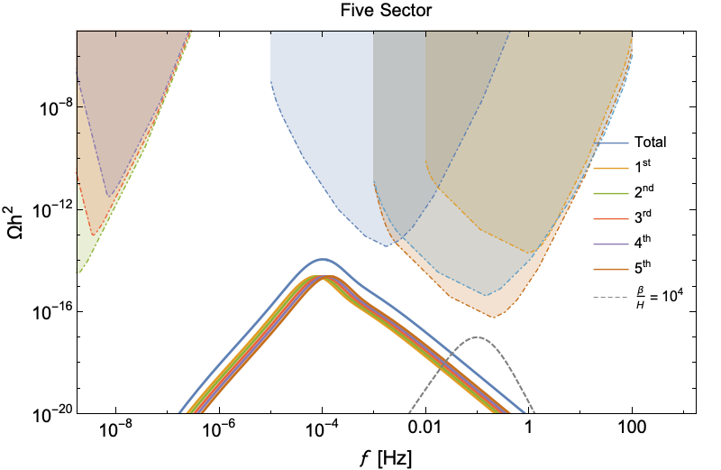
There are four scenarios that we examine, with key parameters presented in Table 1.
- •
Maximized signal: A single additional heavy hidden sector reheated to a temperature that saturates current experimental bounds. The SM photon bath temperature at the time of the hidden sector PT is GeV. In the naturalness framework this is equivalent to reheating a standard sector with up to the maximum allowed temperature ratio.
- •
Large split scenario: A scenario where two additional hidden sectors have been reheated — these sectors have Higgs VEVs that are split by a factor of
(46) This results in a difference in the scale of the SFOPTs leading to the SM photon bath temperature changing a large amount during the time between the PTs. This, in turn, leads to a large separation in the peak frequency of their gravitational wave signals. In the naturalness framework this is equivalent to reheating two standard sectors, one with and another with up to the maximum allowed temperature ratio.
- •
Medium split scenario: Similar to the previous case: these sectors have Higgs VEVs that are split by a factor of
(47) resulting in a much smaller difference in the peak frequency of their gravitational wave signals. In the naturalness framework this is equivalent to reheating two standard sectors, one with and another with up to the maximum allowed temperature ratio.
- •
Five sector scenario: Five sectors are reheated to the maximum allowed temperature ratio, each with VEVs that are
(48) larger than the previous sector.
In all cases where multiple sectors are reheated, we assume for simplicity that all the hidden sectors are reheated to the same temperature.
The GW results of these cases are presented in Fig. 2. In all cases, the summed GW signal is detectable by one or more proposed interferometers. When changing the assumptions on , the scenarios in Fig. 2 are still detectable for values ranging between and . As increases (decreases) the peak frequency moves to higher (lower) frequencies, dictated by Eq. (43), whereas the amplitude decreases (increases) shown in Eq. (41).
The frequency dependence in Eq. (42) takes the form of , this causes a cancellation between the redshifting factors. As multiple sectors phase transition at different times, and therefore different SM photon temperatures, the peaks will shift relative to each other, purely from the linear temperature dependence of the peak frequency given in Eq. (43). This is seen in Fig. 2, where the spectrum peaks are shifted causing a peak broadening of the summed spectrum. The broadening can be substantial if the hidden sectors transition between a large gap of time (temperature). Eventually, a temperature limit will be reached where two (or multiple) distinct peaks will be visible, provided that the amplitudes are comparable.


VI.2 Detection of Stochastic Graviational Waves
A stochastic gravitational wave background could be detectable if the signal-to-noise ratio (SNR) is above some threshold value, , dictated by the capabilities of future interferometers and pulsar timing arrays (PTAs). These interferometers or PTAs quote their experimental sensitivies in terms of spectral noise curves, , which can be translated into units of energy density through . If the experiment uses a single (multiple) detector, the autocorrelated (cross-correlated) SNR is used in comparing to the threshold value . The autocorrelated and cross-correlated SNR are explictly given as Allen and Romano 1999,
| (49) |
where is the exposure time of the experiment. The integration covers the entire broadband range of frequencies . LISA (Audley et al. 2017) and B-DECIGO (Isoyama et al. 2018) are proposed to be single-detector interferometers, whereas BBO (Crowder and Cornish 2005b) and DEICIGO (et al 2017) would be built from an array of multiple interferometers. GW signals produced from an early cosmological phase transition would be seen as a stochastic background. Assuming that the GW follows a power law background in frequency, it is commonplace to quote the power law integrated (PLI) sensitivity curves Thrane and Romano 2013. The PLI curves are constructed using information from the power law form of the signal,
| (50) |
where is the spectral index of the power law, and is an arbitrary reference frequency which has no effect on the PLI sensitivities. is the energy density calculated using Eq. (49) with spectral index and reference frequency . The method of calculating the PLI curves involves plotting , using Eq. (50), for various spectral indices and for some fixed threshold value of . Each curve will lay tangent to the PLI curve, more formally,
| (51) |
The spectral noise curves used to create the PLI curves shown in Figs. 1 and 2 were taken from (Robson et al. 2019; Yagi et al. 2011; YAGI 2013; Isoyama et al. 2018; Breitbach et al. 2018) for the interferometers and (Breitbach et al. 2018; Janssen et al. 2015) for the Square Kilometer Array (SKA) pulsar timing array. We have assumed an observation time of years for the interferometers and years for the various stages of SKA. In the case of the PTA experiments, the sensitivity curves are dependent on how frequently the pulsar’s timing residuals, , are measured. When using Eq. (49) to construct the PLI curves for SKA, the upper integration bound is inversely proportional to pulsar’s timing residual, . In this work, it is assumed that days, but this may underestimate the capabilities of SKA as well as the cadences of the pulsar populations. If the timing residuals are lowered the maximum frequency reach of SKA increases, and the corresponding PLI curves in Figs. 1 2 are shifted to the right, possibly giving the PTAs sensitivity to some of the scenarios considered here.
VII Conclusion
As detection capabilities increase, gravitational wave signals continue to grow in importance as phenomenological signatures that can offer us a unique glimpse into the universe as it was in the early epochs. The space-based interferometers planned for the next generation of GW experiments will be sensitive enough to begin searching for signals of the cataclysmic disruption of space-time due to SFOPT. As we inch closer to these measurements becoming available, it becomes important to develop ways to analyze and understand this data.
Here, we examined scenarios, including naturalness, that involve multiple hidden sectors and calculated the GW profiles present. Our GW projections demonstrate that although naturalness with the reheaton scenario presented in Arkani-Hamed et al. 2016 is not projected to be detectable in the near future, more generalized scenarios with multiple hidden sector SFOPTs are in an observable region and will begin to be probed by next-generation space experiments. Both cases feature important parts of their GW signals in the void between frequencies detectable by pulsar timing arrays and space-based interferometers — providing theoretical impetus for new experiments capable of probing this region of frequency space.
Further, our results provide a framework for understanding and using GW signals in two different ways: first as a unique signal for specific theories featuring multiple SFOPTs and also as a challenge to broaden the understanding of GW detector sensitivity.
In the former case, this demonstrates the power of GW signals to probe deep into the unknown arena of complex hidden sectors. Individual SFOPTs are understood to create GWs that are assumed to follow an approximate power law. If a model predicts the presence of two, five, or more additional sectors, or features a single extra sector with multiple PTs, deviations from a standard power law can occur. The multiple transitions that occur in the models outlined here create signals that follow this trend: although the individual GWs do obey approximate power laws, their sum does not — leading to a unique signal indicating so-called dark complexity. Explicitly, a broadening or distortion of the signal around the peak frequency, precisely where the signal has the most energy, could point to a multi-SFOPT scenario and gently guide us in the direction of multiple hidden sectors.
Shifting to the other part of our framework, our results leads to the question “how well can experiments probe non-power-law signals?” For frequency ranges away from the peak of the total, GW signals the quoted detection thresholds should hold: the signals fall off as a power law to a very good approximation. However, for areas around the peak frequency the answer is less clear; the PLI curves are built under the assumption of a power law. Work has been done Alanne et al. 2019 in examining GW signals using peak amplitudes and peak frequencies as the defining observables: this is rooted in the assumption that GW signals have a model-independent spectral shape around peak frequencies. However, our results indicate that this assumption of model independence cannot hold for all cases: sectors with similar (but different) transition temperatures can create either peak broadening or multihump features that differ significantly from a standard power law shape. This points to the need for future work to better understand where the power law approximation breaks down and how this affects detection prospects for the next generation of GW detectors.
Acknowledgements
We thank Yang Bai, Djuna Croon, Kevin Earl, and Yuhsin Tsai for helpful discussions. P.A.S. and D.L. both thank the 2018 Theoretical Advanced Study Institute in Elementary Particle Physics Program (TASI) for setting up a platform for discussion which seeded the genesis of this project. This work was supported in part by the Natural Sciences and Engineering Research Council of Canada (NSERC). D.L. acknowledges support from the NSERC Postgraduate Scholarships-Doctoral Program (PGS D).
Appendix: Nonrunaway phase transitions
If the phase transition occurs in the nonrunaway regime , the dominant contributions to the GW energy densities are given by the sound wave and MHD components (Breitbach et al. 2018),
| (52) |


The new contributions to the GW energy density take on a different form from Eq. (41) (Caprini et al. 2016),
| (53) |
Unlike the runaway case, we do not assume due to the bubbles reaching a terminal velocity. The MHD efficiency factor is a fraction of the sound waves, . Current simulations have motivated a range of (Caprini et al. 2016), where we take the optimistic case of . Both contributions have unique spectral shapes, given to be (Breitbach et al. 2018),
| (54) |
The MHD energy density has a spectral shape dependent on the Hubble rate at the time of nucleation, . Similar to the scalar spectral shape in Eq. (42), the frequencies are scaled by their respective temperature-dependent peak frequency:
| (55) |
We evolve the frequencies and energy densities with the same redshift factors, Eq. (44) from Sec VI. Fig. 3 shows the sum of the GW energy density for the scenarios in Table 1, but instead for the nonrunaway case, with a terminal velocity of . For this case we see that the spectra tend to be shifted to lower frequencies and are more likely to fall in the gap between the interferometers and the pulsar-based detectors. On the other hand, larger values of increase the typical frequency, so this case becomes more sensitive in some scenarios to values of on the larger end of the considered range.
In the sound wave case, these parameterizations are extracted from simulations with corresponding to a long-lasting sound wave component. For high the transition timescale from sound wave to MHD turbulence is much shorter than the Hubble time. When estimating the model expectations for , we enter a regime at which Eq. (53) may be overestimating the sound wave contribution. Investigations of this regime have been done in (Hindmarsh et al. 2017; Ellis et al. 2018; Ellis et al. 2019). This effect, however, only affects the amplitude of the signal, and our work focuses on the unique spectral shapes that are formed in these models. Therefore we project our results for high in Fig. 3 to motivate the novel spectral profiles.
Finally, we note that because the sound wave and MHD contributions have different spectral shapes, the overall spectrum has a kink at a frequency above the peak. In the top left panel of Fig. 3, we show the two contributions separately in addition to their sum to highlight this effect.
References
- Abbott et al. (2016) B. P. Abbott et al. (LIGO Scientific, Virgo), Phys. Rev. Lett. 116, 061102 (2016), arXiv:1602.03837 [gr-qc] .
- Danzmann (1994) K. Danzmann, in Relativistic astrophysics and cosmology. Proceedings, 17th Symposium, Munich, Germany, December 11-17, 1997 (1994) pp. 481–484.
- Seto et al. (2001) N. Seto, S. Kawamura, and T. Nakamura, Phys. Rev. Lett. 87, 221103 (2001), arXiv:astro-ph/0108011 [astro-ph] .
- Crowder and Cornish (2005a) J. Crowder and N. J. Cornish, Phys. Rev. D72, 083005 (2005a), arXiv:gr-qc/0506015 [gr-qc] .
- Crowder and Cornish (2005b) J. Crowder and N. J. Cornish, Phys. Rev. D 72, 083005 (2005b).
- Harry et al. (2006) G. M. Harry, P. Fritschel, D. A. Shaddock, W. Folkner, and E. S. Phinney, Class. Quant. Grav. 23, 4887 (2006), [Erratum: Class. Quant. Grav.23,7361(2006)].
- Janssen et al. (2015) G. Janssen et al., Proceedings, Advancing Astrophysics with the Square Kilometre Array (AASKA14): Giardini Naxos, Italy, June 9-13, 2014, PoS AASKA14, 037 (2015), arXiv:1501.00127 [astro-ph.IM] .
- Audley et al. (2017) H. Audley et al. (LISA), (2017), arXiv:1702.00786 [astro-ph.IM] .
- Amaro-Seoane et al. (2017) P. Amaro-Seoane et al., arXiv e-prints , arXiv:1702.00786 (2017), arXiv:1702.00786 [astro-ph.IM] .
- et al (2017) S. S. et al, Journal of Physics: Conference Series 840, 012010 (2017).
- Isoyama et al. (2018) S. Isoyama, H. Nakano, and T. Nakamura, Progress of Theoretical and Experimental Physics 2018 (2018).
- Witten (1984) E. Witten, Phys. Rev. D30, 272 (1984).
- Hogan (1983) C. J. Hogan, Phys. Lett. 133B, 172 (1983).
- Hogan (1986) C. J. Hogan, Mon. Not. Roy. Astron. Soc. 218, 629 (1986).
- Turner and Wilczek (1990) M. S. Turner and F. Wilczek, Phys. Rev. Lett. 65, 3080 (1990).
- Caprini et al. (2016) C. Caprini et al., JCAP 1604, 001 (2016), arXiv:1512.06239 [astro-ph.CO] .
- Mazumdar and White (2019) A. Mazumdar and G. White, Rept. Prog. Phys. 82, 076901 (2019), arXiv:1811.01948 [hep-ph] .
- Schwaller (2015) P. Schwaller, Phys. Rev. Lett. 115, 181101 (2015), arXiv:1504.07263 [hep-ph] .
- Jaeckel et al. (2016) J. Jaeckel, V. V. Khoze, and M. Spannowsky, Phys. Rev. D94, 103519 (2016), arXiv:1602.03901 [hep-ph] .
- Addazi (2017) A. Addazi, Mod. Phys. Lett. A32, 1750049 (2017), arXiv:1607.08057 [hep-ph] .
- Hardy (2017) E. Hardy, JHEP 02, 046 (2017), arXiv:1609.00208 [hep-ph] .
- Dienes et al. (2017) K. R. Dienes, F. Huang, S. Su, and B. Thomas, Phys. Rev. D95, 043526 (2017), arXiv:1610.04112 [hep-ph] .
- Tsumura et al. (2017) K. Tsumura, M. Yamada, and Y. Yamaguchi, JCAP 1707, 044 (2017), arXiv:1704.00219 [hep-ph] .
- Acharya et al. (2017) B. S. Acharya, M. Fairbairn, and E. Hardy, JHEP 07, 100 (2017), arXiv:1704.01804 [hep-ph] .
- Bernal et al. (2017) N. Bernal, M. Heikinheimo, T. Tenkanen, K. Tuominen, and V. Vaskonen, Int. J. Mod. Phys. A32, 1730023 (2017), arXiv:1706.07442 [hep-ph] .
- Aoki et al. (2017) M. Aoki, H. Goto, and J. Kubo, Phys. Rev. D96, 075045 (2017), arXiv:1709.07572 [hep-ph] .
- Heikinheimo et al. (2018) M. Heikinheimo, K. Tuominen, and K. Langæble, Phys. Rev. D97, 095040 (2018), arXiv:1803.07518 [hep-ph] .
- Geller et al. (2018a) M. Geller, A. Hook, R. Sundrum, and Y. Tsai, Phys. Rev. Lett. 121, 201303 (2018a), arXiv:1803.10780 [hep-ph] .
- Croon et al. (2018) D. Croon, V. Sanz, and G. White, JHEP 08, 203 (2018), arXiv:1806.02332 [hep-ph] .
- Baldes and Garcia-Cely (2019) I. Baldes and C. Garcia-Cely, JHEP 05, 190 (2019), arXiv:1809.01198 [hep-ph] .
- Bai et al. (2019) Y. Bai, A. J. Long, and S. Lu, Phys. Rev. D99, 055047 (2019), arXiv:1810.04360 [hep-ph] .
- Breitbach et al. (2018) M. Breitbach, J. Kopp, E. Madge, T. Opferkuch, and P. Schwaller, (2018), arXiv:1811.11175 [hep-ph] .
- Fairbairn et al. (2019) M. Fairbairn, E. Hardy, and A. Wickens, JHEP 07, 044 (2019), arXiv:1901.11038 [hep-ph] .
- Helmboldt et al. (2019) A. J. Helmboldt, J. Kubo, and S. van der Woude, (2019), arXiv:1904.07891 [hep-ph] .
- Caputo and Reig (2019) A. Caputo and M. Reig, (2019), arXiv:1905.13116 [hep-ph] .
- Bertone et al. (2019) G. Bertone et al., (2019), arXiv:1907.10610 [astro-ph.CO] .
- Dvali and Redi (2009) G. Dvali and M. Redi, Phys. Rev. D80, 055001 (2009), arXiv:0905.1709 [hep-ph] .
- Arkani-Hamed et al. (2016) N. Arkani-Hamed, T. Cohen, R. T. D’Agnolo, A. Hook, H. D. Kim, and D. Pinner, Phys. Rev. Lett. 117, 251801 (2016), arXiv:1607.06821 [hep-ph] .
- Craig et al. (2015a) N. Craig, S. Knapen, and P. Longhi, Phys. Rev. Lett. 114, 061803 (2015a), arXiv:1410.6808 [hep-ph] .
- Craig et al. (2015b) N. Craig, S. Knapen, and P. Longhi, JHEP 03, 106 (2015b), arXiv:1411.7393 [hep-ph] .
- Chialva et al. (2013) D. Chialva, P. S. B. Dev, and A. Mazumdar, Physical Review D 87 (2013), 10.1103/physrevd.87.063522.
- Dienes and Thomas (2012a) K. R. Dienes and B. Thomas, Phys. Rev. D85, 083523 (2012a), arXiv:1106.4546 [hep-ph] .
- Dienes and Thomas (2012b) K. R. Dienes and B. Thomas, Phys. Rev. D85, 083524 (2012b), arXiv:1107.0721 [hep-ph] .
- Susskind (1979) L. Susskind, Phys. Rev. D20, 2619 (1979).
- Aghanim et al. (2018) N. Aghanim et al. (Planck), (2018), arXiv:1807.06209 [astro-ph.CO] .
- Marsh (2016) D. J. Marsh, Physics Reports 643, 1 (2016), axion cosmology.
- Geller et al. (2018b) M. Geller, A. Hook, R. Sundrum, and Y. Tsai, Phys. Rev. Lett. 121, 201303 (2018b).
- Aoki et al. (2006) Y. Aoki, G. Endrodi, Z. Fodor, S. D. Katz, and K. K. Szabo, Nature 443, 675 (2006), arXiv:hep-lat/0611014 [hep-lat] .
- Bhattacharya et al. (2014) T. Bhattacharya et al., Phys. Rev. Lett. 113, 082001 (2014), arXiv:1402.5175 [hep-lat] .
- Svetitsky and Yaffe (1982) B. Svetitsky and L. G. Yaffe, Nuclear Physics B 210, 423 (1982).
- Pisarski and Wilczek (1984) R. D. Pisarski and F. Wilczek, Phys. Rev. D29, 338 (1984).
- Panero (2009) M. Panero, Phys. Rev. Lett. 103, 232001 (2009), arXiv:0907.3719 [hep-lat] .
- Cui et al. (2012) J.-W. Cui, H.-J. He, L.-C. Lu, and F.-R. Yin, Phys. Rev. D85, 096003 (2012), arXiv:1110.6893 [hep-ph] .
- Tanabashi et al. (2018) M. Tanabashi et al. (Particle Data Group), Phys. Rev. D 98, 030001 (2018).
- Gell-Mann et al. (1968) M. Gell-Mann, R. J. Oakes, and B. Renner, Phys. Rev. 175, 2195 (1968).
- Schwartz (2014) M. D. Schwartz, Quantum Field Theory and the Standard Model (Cambridge University Press, 2014).
- Mangano et al. (2005) G. Mangano, G. Miele, S. Pastor, T. Pinto, O. Pisanti, and P. D. Serpico, Nucl. Phys. B729, 221 (2005), arXiv:hep-ph/0506164 [hep-ph] .
- Abazajian et al. (2016) K. N. Abazajian et al. (CMB-S4), (2016), arXiv:1610.02743 [astro-ph.CO] .
- Trodden and Carroll (2004) M. Trodden and S. M. Carroll, in Progress in string theory. Proceedings, Summer School, TASI 2003, Boulder, USA, June 2-27, 2003 (2004) pp. 703–793, [,703(2004)], arXiv:astro-ph/0401547 [astro-ph] .
- Fodor and Katz (2002) Z. Fodor and S. D. Katz, JHEP 03, 014 (2002), arXiv:hep-lat/0106002 [hep-lat] .
- Linde (1983) A. D. Linde, Nucl. Phys. B216, 421 (1983), [Erratum: Nucl. Phys.B223,544(1983)].
- Espinosa et al. (2010) J. R. Espinosa, T. Konstandin, J. M. No, and G. Servant, JCAP 1006, 028 (2010), arXiv:1004.4187 [hep-ph] .
- Grojean and Servant (2007) C. Grojean and G. Servant, Phys. Rev. D 75, 043507 (2007).
- Kosowsky et al. (1992) A. Kosowsky, M. S. Turner, and R. Watkins, Phys. Rev. D 45, 4514 (1992).
- Huber and Konstandin (2008) S. J. Huber and T. Konstandin, Journal of Cosmology and Astroparticle Physics 2008, 022 (2008).
- Hindmarsh et al. (2014) M. Hindmarsh, S. J. Huber, K. Rummukainen, and D. J. Weir, Phys. Rev. Lett. 112, 041301 (2014).
- Caprini and Durrer (2006) C. Caprini and R. Durrer, Phys. Rev. D 74, 063521 (2006).
- Bödeker and Moore (2017) D. Bödeker and G. D. Moore, Journal of Cosmology and Astroparticle Physics 2017, 025–025 (2017).
- Kamionkowski et al. (1994) M. Kamionkowski, A. Kosowsky, and M. S. Turner, Phys. Rev. D 49, 2837 (1994).
- Thrane and Romano (2013) E. Thrane and J. D. Romano, Phys. Rev. D 88, 124032 (2013).
- Allen and Romano (1999) B. Allen and J. D. Romano, Phys. Rev. D 59, 102001 (1999).
- Robson et al. (2019) T. Robson, N. J. Cornish, and C. Liu, Classical and Quantum Gravity 36, 105011 (2019).
- Yagi et al. (2011) K. Yagi, N. Tanahashi, and T. Tanaka, Phys. Rev. D 83, 084036 (2011).
- YAGI (2013) K. YAGI, International Journal of Modern Physics D 22, 1341013 (2013).
- Alanne et al. (2019) T. Alanne, T. Hugle, M. Platscher, and K. Schmitz, “A fresh look at the gravitational-wave signal from cosmological phase transitions,” (2019), arXiv:1909.11356 [hep-ph] .
- Hindmarsh et al. (2017) M. Hindmarsh, S. J. Huber, K. Rummukainen, and D. J. Weir, Phys. Rev. D96, 103520 (2017), arXiv:1704.05871 [astro-ph.CO] .
- Ellis et al. (2018) J. Ellis, M. Lewicki, and J. M. No, (2018), 10.1088/1475-7516/2019/04/003, [JCAP1904,003(2019)], arXiv:1809.08242 [hep-ph] .
- Ellis et al. (2019) J. Ellis, M. Lewicki, J. M. No, and V. Vaskonen, Journal of Cosmology and Astroparticle Physics 2019, 024 (2019).