A Polyhedral Homotopy Algorithm For Real Zeros
Abstract.
We design a homotopy continuation algorithm, that is based on Viro’s patchworking method, for finding real zeros of sparse polynomial systems. The algorithm is targeted for polynomial systems with coefficients satisfying certain concavity conditions, it tracks optimal number of solution paths, and it operates entirely over the reals. In more technical terms; we design an algorithm that correctly counts and finds the real zeros of polynomial systems that are located in the unbounded components of the complement of the underlying A-discriminant amoeba. We provide a detailed exposition of connections between Viro’s patchworking method, convex geometry of A-discriminant amoeba complements, and computational real algebraic geometry.
Key words and phrases:
-discriminant, Amoeba, Entropy, Fewnomial theory, homotopy continuation, Viro’s Patchworking2010 Mathematics Subject Classification
14P05, 14P25, 14T05, 68R05, 52B11, 65D99, 65Y201. Introduction
Let be a system of sparse polynomials in with support sets . More precisely, let
where . Bernstein’s theorem from 1975 [Ber75] shows that for generic choice of coefficients of the number of zeros of on equals to the mixed volume of the Newton polytopes .
In the early 90’s the polyhedral homotopy method was developed as an algorithmic counterpart of Bernstein’s theorem [HS95]. The main idea of the polyhedral homotopy method is to continuously deform a given polynomial system to another “easy” system, that can be solved by pure combinatorics, and then trace back the change in the solution set with numerical path trackers. This geometric idea is colloquially referred to as toric deformation, and the “easy” systems with combinatorial structure are referred to as the systems at the toric limit. Polyhedral homotopy method is currently implemented in several packages such as PHCPack [Ver99], Hom4ps-3 [CLL14], pss5 [Mal19], and HomotopyContinuation.jl [BT18], and it has remarkable practical success.
For most applications of polynomial system solving, and for certain questions in theoretical computer science one needs to count and find zeros of polynomial equations over real numbers, e.g. see [JS17, Koi10]. No general and efficient algorithm that counts real zeros of arbitrary sparse polynomial systems is known, and there are good complexity theoretic reasons to believe that at this level of generality the problem is intractable. Our aim is to locate a sufficiently general and tractable sub-case of real zero finding problem: Consider support sets are given, can we find effectively checkable conditions on the coefficients of the equations that guarantee tractable solving over the reals? In other words: Where are the “easy” equations located in space of sparse real polynomial systems with equations and unknowns?
An important observation from real algebraic geometry suggests a map for “easy” polynomial systems: one can count real zeros by pure combinatorics if the polynomial system is at the “toric limit”. We informally state this result ( Viro’s Patchworking Method for Complete Intersections) to motivate our discussion; see section 2.2 for a precise statement.
Theorem 1.1 (Viro’s Patchworking Method for Finitely Many Zeros).
Let , let be lifting functions, and consider the following family of equations parametrized by :
Let be the sign functions defined by signs of the coefficients . Then, for sufficiently large , the set of common zeros of on is homeomorphic to
where are the positive part of tropical varieties as defined in section 2.2 .
theorem 1.1 yields a polyhedral object that is homeomorphic to the common zero set of on for sufficiently large , and it can also be used to handle the set of common zeros on . We have three immediate questions:
- (1)
How can we quantify precisely when is “sufficiently large”?
- (2)
Given a polynomial system with support sets and coefficients for (as in the theorem statement), can we guarantee that the number of common real zeros does not change as goes from to ?
- (3)
Can we use the technique in theorem 1.1 for polynomial systems that are not necessarily at the “toric limit”?
The first two questions are interrelated, and they form the main difficulty with respect to developing an algorithmic version of theorem 1.1. These questions were asked since 90’s [Stu98]; to the best of our knowledge the current paper provides the first progress. We provide an explicit criterion to answer the second question (stated in section 3). The criterion also furnishes a homotopy algorithm that operates entirely over the reals, which we call real polyhedral homotopy algorithm (RPH).
The third question is due to Itenberg and Roy; they conjectured Viro’s patchworking method provides an upper bound for the number of real zeros regardless of the polynomial system being at the toric limit or not [IR96]. Li and Wang provided a counterexample to the Itenberg-Roy Conjecture [LW98].
1.1. Effective Patchworking
Our development is based on an observation from the book [GKZ08] by Gelfand, Kapranov, and Zelevinsky (henceforth GKZ) which provides a link between Viro’s patchworking method and -discriminants. Using the GKZ observation for an algorithm is not straightforward. It requires to locate a query point against the -discriminant variety, and this may be intractable: The defining equation of the discriminant locus is known to be extremely complicated; it obstructs the use of computational algebra methods. However, it is no obstruction against the use of amoeba theory. Discriminantal amoebas are proven to admit a certain parametric description, and it is easy to compute normal directions on their boundary; see section 2.9. We exploit these special differential geometric properties of -discriminant amoebas to develop an effective criterion for checking whether a given polynomial system is “easy”. Note that RPH relies on notions from discrete and tropical geometry, and on further notions from GKZ. Furthermore, we use an algorithm called Tropical Homotopy due to Jensen [Jen16b]. So, before reading the main statement in section 3 we encourage the reader to check familiarity with the content of section 2.1, section 2.2, section 2.3, section 2.7, and section 2.9.
1.2. Complexity aspects
Our work is inspired by the practical efficiency of complex polyhedral homotopy algorithm. Complexity aspects of polyhedral homotopy have been elusive for more than two decades; early papers did not include any complexity analysis, later different authors approached the issue [MR04, Mal17, Mal16], certain technical obstacles still remain; see section 5.4.
A complete complexity analysis of RPH will only become possible when the scientific community fully understands the complexity of numerical path tracking for sparse polynomial systems. We present our thoughts on the complexity of discrete computations, and touch upon the complexity of the numerical part of RPH in section 5.
We point out here that the main parameters governing the complexity of RPH are different than its complex cousin: the overall complexity of RPH is controlled by the number of mixed cells (a combinatorial quantity), the complexity of complex polyhedral homotopy is, in contrast, controlled by the mixed volume (a geometric invariant).
1.3. Connections to fewnomial theory
A system of polynomials is called a patchworked polynomial system if the real zero set of is homeomorphic to a simplicial complex created by Viro’s combinatorial patchworking technique. For instance, every polynomial system that passes our test in section 3 is a patchworked system. In section 5.3 we observe the following result that is reminiscent to a conjecture from fewnomial theory [Kho91] attributed to Kushnirenko [Kus].
Theorem 1.2.
Let be a patchworked polynomial system where every polynomial has at most terms. Then can have at most many common zeros on .
Note that where the right hand side resembles Kushnirenko’s conjecture. To illustrate the difference between the number of paths tracked in RPH and the number of paths in complex polyhedral homotopy we provide a very simple example.
Example 1.3.
Let , and let where are real polynomials with three variables. Further assume that the coefficients of is generic in the sense of Bernstein’s theorem, this implies has many zeros on . If is a patchworked polynomial system, by Theorem 1.2 it has at most zeros in . We should note that is very much an over estimation (correct bound in this specific example is at most ) where else , with being arbitrarily large, is the exact number of zeros in . ∎
theorem 1.2 is a direct application of McMullen’s upper bound theorem. Things become geometrically more interesting when one tries to bound the number of mixed cells for support sets with different cardinalities (mixed supports). In [Bih16] it is claimed that a patchworked polynomial system , where has at most many terms, can have at most many zeros on . We have learned from Bihan that the proof of this result is not correct, but the result still holds true. Bihan informed us that a new proof and an erratum will appear soon ([Bih20]).
1.4. Structure of the paper
Our aim is to write this paper as self contained as possible. The preliminaries section contains background information and results from discrete geometry, the theory of -discriminants, symbolic computation, and numerical path trackers. Jensen’s tropical homotopy algorithm and mixed cell cones are also introduced in this section. In the third section, we transform asymptotic and qualitative results from [GKZ08] to a more quantitative and checkable condition. In the fourth section we present our real polyhedral homotopy algorithm and an example. The fifth section is concerned with the complexity aspects. The last section contains a discussion of questions, that were brought to our attention after the initial version of this paper appeared on ArXiv.
Acknowledgments
We cordially thank Sascha Timme for implementing a preliminary version of the algorithm developed in this article in the software HomotopyContinuation.jl, and for his help with developing 4.1. We thank Matías Bender, Paul Breiding, Felipe Cucker, Mario Kummer, Gregorio Malajovich, Jeff Sommars, and Josue Tonelli-Cueto for useful discussions. The first author thanks J. Maurice Rojas for introducing him to the beautiful book [GKZ08]. First author is supported by NSF CCF 2110075, and the second author is supported by the DFG grant WO 2206/1-1.
2. Preliminaries
We denote , , and . Let denote the -th coordinate vector in . To avoid redundancies later in the articles we set .
For a given convex set , we denote its boundary by . For a convex cone , the dual cone is defined as
For a given polytope , we denote its vertex set as . For the normal cone is the collection of linear functional that achieves its maxima over at and is denoted with . Entire collection of all normal cones form a fan called normal fan and denoted with .
In what follows we consider finite sets and , which are support sets of polynomials. We denote the Minkowski sum of the as . Note that
For a polynomial with support , the Newton polytope is given by . We denote the variety, i.e. the common solutions of a system of polynomials on complex numbers as , the real locus as , and positive / nonzero real locus as and .
2.1. Polyhedral subdivisions, secondary polytope and Cayley configuration
In this section we introduce polyhedral subdivisions, secondary polytopes and Cayley configurations; for further details we refer the reader to [DLRS10].
Let be a set of lattice points and let be a function. The lifting of induced by is defined as:
We call a face of an upper face if it is given by
where is a vector with a positive last entry. Intuitively, upper faces are the faces that are “visible” from . We project upper faces of on the point set :
is a polyhedral subdivision of . Polyhedral subdivisions obtained this way are called coherent or regular. Note that is a triangulation (i.e. a subdivision using only simplices) unless the lifted points have certain affine dependencies [DLRS10, Remark 5.2.3].
Now we define the secondary polytope of , which encodes all coherent triangulations of , and discuss its key properties; see [DLRS10, Section 5].
Definition 2.1.
Let be a triangulation of , and let be the simplices in . We define
We define the secondary polytope of as:
The corresponding normal fan is called the secondary fan. For its cones, the secondary cones, we use the abbreviated notation . ∎
Theorem 2.2.
[DLRS10, Section 5]. The secondary polytope has the following properties:
- (1)
The vertices of are in one to one correspondence to the coherent triangulations of .
- (2)
The face lattice of is isomorphic to a refinement poset of the coherent polyhedral subdivisions of .
- (3)
A lifting function induces the triangulation if and only if .
- (4)
Consider the support set as a integer matrix. Then every secondary cone includes the dimensional linear space spanned by rows of and all ones vector . As a consequence, the secondary polytope is dimensional.
For later use, we need to have a better understanding of the description of secondary cones . We first define a circuit.
Definition 2.3.
An affine dependence among lattice points of a set is the relation given by where . A circuit is a collection of affinely dependent lattice points where every proper subset of is affinely independent. Consequenlty, circuit represents a unique (up to scaling) affine relation and ∎
A rhombus in the plane is a nice example of a circuit. The following is a basic fact about circuits, see e.g. Lemma 2.4.2 [DLRS10].
Lemma 2.4.
Let be a circuit, then can be decomposed into a disjoint union of two sets with the following property:
are the two triangulations of .
The volume of the simplex is equal to absolute value of a determinant. Let us denote this determinant with . A standard argument, see e.g. Remark 4.1.8 in [DLRS10], shows that ’s determine the unique affine relation supported by . That is, using the terminology in 2.3, we have (up to swapping and ).
Now consider a regular triangulation and suppose is a lifting function that induces . Then, for a simplex in , and with , we must have that lies ‘above’ the affine spane of . Suppose is the unique affine relation of the circuit , if we have then we know that is in the affine span of the vectors . To have ‘above’ simply corresponds to . In conclusion, the secondary cone is described by inequalities supported on circuits, and these inequalities are of the form where are signed volumes of simplices in the triangulation of the circuit (up to scaling).
Now we consider polyhedral subdivision of a set where . Let be a cell in coherent polyhedral subdivision of introduced by a lifting function . Then corresponds to a face in . Let where are the corresponding faces on .
Definition 2.5.
A coherent polyhedral subdivision of for is called fine mixed if it satisfies the following conditions:
- (1)
For all cells in the subdivision, we have , and
- (2)
for all cells in the subdivision we have ,
where denotes the number of vertices of . ∎
We also need to define Cayley configuration of point sets and the corresponding Cayley polytope.
Definition 2.6.
We define the Cayley configuration of as
The Cayley polytope is defined as , denoted by . ∎
The following observation is implicit in most papers in literature: A natural slicing of the Cayley polytope is equivalent to . More precisely, consider the following set defined by the intersection of with several hyperplanes:
Observe that a -scaling of , i.e., , is equal to . For a detailed explanation and a picture-proof see [HRS00].
Suppose that is a coherent triangulation of the Cayley configuration . First, note that creates a polyhedral subdivision of . Via the equivalence, this gives a polyhedral subdivision of . Let be a simplex in , then has vertices which split into sets of vertices that are induced by . None of the are empty since otherwise can not be full-dimensional. Then, up to an isomorphism, yields a cell in the polyhedral subdivision of , and all such cells yield a fine mixed subdivision of . This correspondence gives a bijection between coherent triangulations of the Cayley polytope and coherent fine mixed subdivisions of the Minkowski sum ; see [Stu94a, Theorem 5.1].
In summary, coherent fine mixed subdivisions of are encoded by the vertices of the secondary polytope and the corresponding secondary cones.
Remark 2.7.
At various parts of this article (in our theorem statements and algorithms) we work with triangulations. For a generic lifting function the induced polyhedral subdivision is a triangulation. The proof of [DLRS10, Proposition 2.2.4] suggests an algorithm, albeit an inefficient one, to check whether a given lifting is generic. The question of finding an efficient algorithm to check genericity of a lifting is an interesting question, but it lies beyond the scope of our paper.
2.2. Viro’s patchworking method
In this section we introduce Viro’s patchworking method for complete intersections. For further details and relations to Hilbert’s 16th problem, we kindly refer the reader to Viro’s survey [Vir08]. For further background information on tropical geometry see e.g., [MR09, IMS09, MS15]. For implementations of patchworking technique please see [OKdW18] and [JV20].
Definition 2.8.
Let and be a coherent triangulation of given by a lifting function . We define the associated tropical variety as
∎
Since we are interested in real varieties, we need to distinguish a positive and a negative part of . Observe that together with its complement creates a polyhedral decomposition of . Also, by definition, every full-dimensional cell in the complement of corresponds to a unique as it is given by the set:
We define the sign of this cell as . For every -dimensional cell in , there exist two adjacent -dimensional cells with signs assigned by . This motivates the definition of the positive part of a tropical variety.
Definition 2.9.
The positive part of a given tropical variety is the subcomplex consisting of those -dimensional cells that are adjacent to two -cells with different signs. ∎
Theorem 2.10 (Viro’s Patchworking for Complete Intersections [Stu94b]).
Let , let be a lifting function. Consider a system of polynomials defined as follows:
with . Let be the sign function defined by coefficients of . Then, for sufficiently large , the real algebraic set is homeomorphic to
where and are restrictions of and to .
Remark 2.11.
For readers who are familiar with non-Archimedian tropical geometry the theorem statement here might look confusing. The only difference is that in non-Archimedian tropical geometry it is customary to use min notation, lower facets, and tends to zero. In amoeba theory, however, it is customary to use max notation, upper facets, and tends to . We follow the amoeba theory convention.
theorem 2.10 generalizes to the set of zeros on the appropriate toric variety by applying the theorem on every one of the orthants separately and then gluing them together; see [Stu94b, Theorem 5]. We illustrate theorem 2.10 on the most simple example possible.
Example 2.12.
The set represents the support set for linear forms (and hence its convex hull is the standard simplex). We consider positive solutions of an affine linear form , i.e., the solutions with . We use a variant of moment the from symplectic geometry called algebraic moment map:
This map is a homeomorphism. The image of under is given by:
Hence, is defined by the linear form on the simplex , and it separates those with from those with . ∎
To prove theorem 2.10 above, one replaces the simplex with the triangulation, and the moment map with the moment map corresponding to the toric variety defined by as explained in of [GKZ08, Chapter 11, Section 5, Subsections C and D]. We provide another example, first considered by Sturmfels [Stu94a, Page 382].
Example 2.13.
Consider the two polynomials
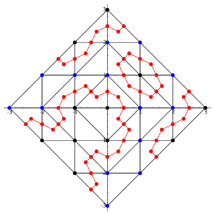
We consider the lifting function introduced by the exponents of , the sign function introduced by the coefficients of and , and compute the corresponding patchworking. We present the outcome in fig. 1. The computation was already carried out by Sturmfels in the original article [Stu94a] in ’94. Here, we generate a plot using the Viro.sage package by O’Neill, Kwaakwah, and the second author [OKdW18]. ∎

2.3. Mixed-cell cones and Jensen’s tropical homotopy algorithm
In this article we are concerned with zero dimensional systems, that is we have support sets . For this case, some cells in the regular triangulation (introduced by a lifting ) of are of particular interest. These cells are called mixed cells. Formally, a cell that has elements from each is called a mixed cell. Equivalently, after identification as explained section 2.1, in a fine mixed subdivision of , mixed cells are the cells that are given by the Minkowski sum of edges.
On the dual side, when we consider the finite set of points in the intersection
each of these points correspond to a mixed cell in the triangulation of where every two vertices from each have opposite signs. In the current literature, such a simplex is called an alternating mixed cell [Jen16b].
The main observation here is that theorem 2.10 depend only on the mixed cells in a triangulation of ; we do not need to differentiate between two triangulations that have same collection of mixed cells. We formalize this as follows.
Definition 2.14 (Mixed-Cell Cone of a Triangulation).
Let be a triangulation of , and let be a mixed cell. For every lifting function (represented by a vector in ) we denote the induced subdivision as . We define the mixed cell cone of as:
Moreover, we define the mixed cell cone of as:
∎
To clarify the difference between the mixed cell cone and the secondary cone we make a definition and state a lemma.
Definition 2.15.
Let and set . If is a facet of defined by for some , or then we call an irrelevant facet. If is a face included in an irrelevant facet, we call an irrelevant face. ∎
Lemma 2.16.
Let for a lifting function , and assume that where is a vertex of the Newton polytope of the -discriminant and is its normal cone. Then, we have
Moreover, if then is supported on a set that is included in the union of irrelevant faces of .
Proof.
Inclusion of the cones follow directly from definition, for further structural information we refer to -equivalence notion in Chapter 11, Section 3, subection B of [GKZ08].
We prove “moreover” part of the claim. Let be an inequality supported on a circuit . We claim in there exist an such that . Assume otherwise, then we have that for some : for all , and . Then, passing from one triangulation of to another involves a mixed cell change which contradicts with the assumption . Now without loss of generality assume . Then lies in an irrelevant face of , and the lattice distance from to affine hull of is . One can easily observe that the simplex corresponding to in is not full-dimensional and hence has volume zero. Thus, the inequality is supported on . In general, any element of is a conic combination of circuit inequalities and we showed that such are supported on irrelevant faces. ∎
In the rest of this paper we will use the mixed-cell cone and it will be represented by circuit inequalities generating the cone, that is we work with . Luckily for us, there is already an efficient algorithm for computing : Jensen’s tropical homotopy algorithm, see [Jen16b], computes for a given (generic) lifting function , and point configurations , the triangulation of and . The idea of Jensen’s algorithm is to start from a lifting function yielding only one mixed cell. Then, one keeps track of the changes in the mixed-cell cone as one changes the lifting function linearly from to a target lifting . The algorithm updates the mixed-cell cone with the violated circuit inequalities, and halts whenever it arrives at a triangulation with . The correctness of the algorithm follows from the fact that changes in the regular triangulations always happen by a change between two triangulations of a circuit, and every such change corresponds to one circuit inequality added to the mixed-cell cone.
2.4. Solving binomial systems over the reals
Since we repeat the Viro construction in every orthant of , the sign vector changes. However, the lifting function and the corresponding triangulation remains the same for all orthants. So, in order to count the number of real zeros with Viro’s method, one needs to investigate the mixed cells and check how many times a mixed cell becomes an alternating one. Algorithmically, instead of going through Viro’s construction times, it is more convenient to use binomial systems, i.e., systems of polynomials where every polynomial has only two terms. Every mixed cell corresponds to a binomial system, and solving that binomial system on corresponds to counting how many times the mixed cell becomes and alternating mixed cell. This approach is much more effective.
Now we outline how to solve binomial systems over the reals. Consider the following system of binomials:
where and . This system is equivalent to the following system of equations:
| (2.1) |
Set , and . To solve the system eq. 2.1 over , it suffices to perform the elementary integer operations that reduce into its Hermite normal form. This operations can be done in strong polynomial time [KB79]. The result is a system of equations in the following format:
| (2.2) |
where and . The solutions of eq. 2.2 are completely determined by the signs of and being even or odd. Hence, eq. 2.2 either has no solution in , or there exist solutions differing only by their signs.
There is also a recent paper focusing on probabilistic analysis of numerical methods for binomial system solving [PPR19].
2.5. -discriminants
Given a set of lattice points , we define
as the space of polynomials supported on . Note that is isomorphic to with . We define analogously with . Now we define our protagonist the -discriminant variety:
is a cone over a projective variety, to get a better sense of this we need to introduce projective toric variety corresponding to :
One can observe that is essentially Zariski closure of a torus orbit. A polynomial supported on can be considered as a linear form on the toric variety . Discriminant variety corresponds to the hyperplanes that intersect the toric variety non-transversally. This means if then the zero set of has no singularity on . This also means is the cone over the projective dual of . Thus, except for specific degenerate configurations , is an irreducible hypersurface given by a polynomial with integral coefficients; [GKZ08, Chapter 9]. We denote the defining equation of with . We are interested in the real part of the discriminant variety
The hypersurface partitions the coefficient space into connected components. If two polynomials lie in the same connected component of and is smooth then the zero sets of and on are isotopic on [GKZ08, pg 380].
For the purposes of homotopy continuation we want to have zero sets of be isotopic in the torus orbit instead of the compactification . The nice fact is that admits a decomposition into a disjoint union of torus orbits:
where are faces of the polytope and denotes the torus orbit for which the toric variety is the closure. So to have and isotopic we will require two conditions: and both does not have a zero on for any proper face of , and and are isotopic on . Since singularities of toric variety are known to be on for co-dimension two or higher faces, once the first condition is guaranteed the second condition boils down to and being in the same connected component in .
At this point, we need to introduce sparse resultant. We summarize basic properties in the following proposition-definition.
Proposition 2.17.
[GKZ08, Chapter 8] Let be a collection of finite sets. Then there exists a polynomial with the following properties:
- •
has integral coefficients and it is irreducible.
- •
If is a polynomial system with and has a zero in , then .
An exposition for sparse resultants with a computational focus can be found in [CE00]. A nice trick referred to as “Cayley trick” relates -discriminants and sparse resultants.
Lemma 2.18.
[GKZ08, Chapter 9, Prop 1.7] Using the notation of proposition 2.17 and letting , we have
where denotes the new variables added in the construction of .
Now we would like to think about singular zeros of a sparse polynomial system. For a tuple of coefficient vectors with , let be the polynomial system with . We define the discriminantal locus for systems of equations as follows:
The toric variety that is dual to may not be clear at first sight, but it is isomorphic to ; we refer the reader to [GKZ08, Chapter 8, Proposition 1.4] for a nice explanation.
The discriminantal locus corresponding to hypersurfaces supported by the Cayley configuration is then given by
If is not degenerate, then is an irreducible hypersurface. Also, by using the definition of singularity with the Jacobian matrix, it immediately follows that . The following result of Esterov, proved by a simple perturbation argument, relates and ; see of [Est10, Lemma 3.36], and note that in Esterov’s notation is denoted by .
Theorem 2.19 (Esterov).
If is not defect, and for , then is irreducible of codimension one.
Hence, if the assumptions of Esterov’s theorem are satisfied, then and coincide. So, in order to control the changes in the topology for systems of equations supported with , we use the hypersurface .
2.6. Basics of amoeba theory
In this section, we introduce the notion of amoeba following Gelfand, Kapranov, and Zelevinsky [GKZ08]. For an overview of amoeba theory please see [Mik04, PT05].
Definition 2.20.
We define the Log-absolute value map as
For a Laurent-polynomial and variety we define the amoeba of as . ∎
Lemma 2.21.
Let be a polynomial with support . Let be a vertex of . Suppose that with
for all . Then, .


The statement is well-known; see [GKZ08, Prop. 1.5, Page 195]. Here, we provide the main argument of the proof for the convenience of the reader.
Proof.
We have
Set . Then for a given if this immediately implies and hence . The rest of the proof is straightforward. ∎
lemma 2.21 shows that for every of the there is an unbounded connected component in the complement of the amoeba that includes a copy of the normal cone . The following are the basic facts: these connected components are distinct for every , these connected components exhaust the list of unbounded components in the complement of , and these connected components are convex [PST05, PT05].
2.7. Real toric deformation
This section is to set up the real homotopy starting from combinatorial patchworking to our target system. We will require the deformation path to lie outside of a region given by a union discriminant amoebas. This will ensure there are no root paths that visit toric infinity and that the deformation preserves the geometry of the real zero set.
Proposition 2.22.
Let be point configurations with for all , and let be the Cayley configuration. Suppose that and are vectors with the following properties:
- (1)
is not on the boundary of any secondary cone of the point configuration .
- (2)
For every face of , except for the irrelevant faces, the ray for does not intersect the amoeba of .
We consider a system of equations :
| (2.3) |
Then the real Puiseux series
| (2.4) |
is a solution to the system only if is an outer normal to a lower facet of
where stands for the lifting of with respect to . Moreover, are isotopic for all .
Remark 2.23.
We note that in the statement we have for , and also for ; these two represent the same parameter regime as .
Proof.
The statement about the Puiseux series follows the same proof as [HS95, Lemma 3.1], so we just list the main steps: Put eq. 2.4 into eq. 2.3, divide by the lowest degree term, and set . The system of equations obtained this way will have at most terms in total, and it can have a common zero only if it is a system of binomial equations. On can observe that under -map the solutions of these binomial equations correspond to the finite number points given by Viro’s method. We had already discussed in section 2.3 and section 2.4 that these points given by Viro’s method identify alternating mixed cells.
Now we consider the statement about isotopy. Let . We recall that and are equivalent up to scaling, see section 2.1. Let be a proper face of that is not irrelevant, let be the face of equivalent to , and suppose where is a face of . Observe that . By lemma 2.18, if a polynomial system satisfies then has no zero on . Thus if for all proper faces, except the irrelevant ones, then has no zero on .
The ray does not intersect the amoeba of for any . This implies for all faces , except irrelevant ones, and also for all . So the condition guarantees non-existence of zeros on , and since we have that the zero sets are isotopic on . Thus, are isotopic for all . ∎
2.8. Numerically tracking a solution from toric infinity
The numerical part of our algorithm tracks real zeros of , as in proposition 2.22, from to . There are several technicalities to be careful about: 1-) we are not able to start the homotopy continuation precisely at since all its zeros lie at toric infinity, 2-) we need to design an algorithm to track the solution paths , as in proposition 2.22, from to .
The first issue is theoretically handled by an analytic continuation argument on toric compactification, and it is practically handled by predictor-corrector methods in numerical analysis. The second part, tracking the solution paths, can be done in two ways:
- (1)
trace the solution curves numerically, or
- (2)
start a homotopy from with zeros given by alternating mixed cells and track the solution path from to .
Explaining details of these numerical schemes have the potential of doubling the size of our paper and the techniques are now folklore, so we prefer to have a brief account. An established reference for curve tracing approach, i.e., the first method, is [AG12]. The curve tracing approach is often fast, and it is a standard technique in numerical analysis that is deployed in many applications. However, to the best of our knowledge, the safeguards to control precision issues for standard path trackers only exist for specific cases. The second approach has a well developed theory to control precision issues and conduct rigorous complexity analysis in the case of dense polynomials [BC13]. For sparse polynomials, Malajovich recently developed a theory that allows to express complexity of numerical tracking with certain integrals of condition numbers [Mal16]. We briefly explain Malajovich’s approach in section 5.4. Our algorithm can be implemented using any of the two ways depending on the preferred trade-off between rigor and speed. For a nice exposition on comparing the two alternatives we suggest [BS11a, Section 2.3 and 2.4].
2.9. An entropy type formula for the discriminant locus
In this section, we introduce useful facts about -discriminants, mostly relying on [GKZ08, Chapter 9, Section 3, subsection C] and works of Passare and Tsikh [PT05].
Theorem 2.24 (Horn-Kapranov Uniformization).
Let be a collection of lattice points in , let be the corresponding -discriminant variety. We consider as a matrix, and define
Then admits the following parametrization:
Now consider the amoeba of :
where denotes the Minkowski sum.
It is easy to observe that corresponds to the row span of . Moreover, for any with any scalar multiple of satisfies the same equations. This -dimensional row span and one dimensional linear space represents homogeneities that are present in the discriminant variety; the variety is invariant under torus action and scaling.
For a given hypersurface consider all points which are critical under the map. The -image of these points is called the contour of the corresponding amoeba ; see e.g., [PT05]. It is straightforward to show that the contour contains the boundary , but does not coincide with it in general; see e.g., [PT05]. Moreover, for a real polynomial , the contour contains the amoeba of the smooth part of the real variety, i.e. [PT05].
Let be a Gale dual of , i.e, an integer matrix that has all column sums to be and satisfies . Then, for any with and one can find a with .
It follows from the discussion in [PT05] (see the section titled Discriminants and Real Contours, and specifically Theorem 4), that the parametrization of the contour of the reduced -discriminant amoeba is given as follows:
| (2.5) |
Using eq. 2.5 and the fact that contour includes the amoeba of the real part of the variety, one can concisely write
| (2.6) |
Using the row space of to parameterize the set , this can also be written as follows:
| (2.7) |
where the denote the rows of . As a next step, we define the following map:
The facts listed follows from [GKZ08, Chapter 9, Section 3, subsection C]:
- (1)
The map is -homogeneous, that is for every and we have
- (2)
The image of the map is a hypersurface, and if the Gauss map is defined at then we have
The first property follows since the column sums of equals . The second property is proved by Kapranov [Kap91]. Now assume that we have a , and we would like to write down the equation of the tangent hyperplane at .
Since we know the image under the Gauss map (i.e., the normal direction), we obtain:
One can rewrite this as follows:
| (2.8) |
3. Effective Viro’s Patchworking
Consider a polynomial system with support sets and the coefficient vector . How do we decide if the common real zero set of (up to continuous deformation) can be described by Viro’s patchworking method? Here we present a way to certify if this is the case for a given system : We search for a ray that does not intersect the discriminant amoebae for all faces of , except the irrelevant ones. This represents a real toric deformation starting from as in proposition 2.22.
3.1. Statement of main result and an example
We keep the notation from section 2.9, what follows is the main result of this section.
Proposition 3.1.
Let be a system of sparse polynomials with coefficient vector and support sets where for all . Let be the triangulation of the Cayley configuration that is introduced by using as a lifting function. Let be the corresponding mixed cell cone, and suppose that the dual cone is generated by vectors . Then, if
| (3.1) |
for all , the system is a patchworked polynomial system. Furthermore, for any the ray for does not intersect the amoeba of for all faces of except for the irrelevant ones.
Note that, for any coefficient vector with corresponding triangulation , if the generators of the dual mixed cell cone are for , then, by definition,
for all . To apply proposition 3.1, we need
Here is a normalization; one can just use normalized generators with unit -norm. So the loss in our relaxation is represented by the logarithmic term .
Let us illustrate proposition 3.1 on the simplest case: univariate polynomials. Let , and let . Here a triangulation is subdivision of the interval into a union of smaller sub-intervals . Suppose the lifting function introduces the triangulation . The first “simplex” being means for every with we must have lying above the line segment . In terms of circuit inequalities, this means the following
Or, equivalently
The hypothesis of proposition 3.1 amounts to
If the hypothesis of proposition 3.1 is satisfied for all the circuit inequalities of the triangulation (that is all generators of ) then the number of real zeros of can be counted as follows: Let represent the signs of , set
and let be the number of sign changes in the vector . The vector represents the signs relevant to the triangulation , and due to nature of we have the same sign vector on“negative orthant” . Then proposition 2.22 combined with proposition 3.1 says has many real zeros.
3.2. Some basic results on the complement of -discriminant amobea
For simplicity, we let . Note that . Here we assume the reader is familiar with the basic facts from section 2.6 and start with the following lemma.
Lemma 3.2.
Let be a vertex of the Newton polytope of , and let be the corresponding connected component in the complement of the -discriminant amoeba.
- (1)
Let and let then the ray for does not intersect the -discriminant amoeba.
- (2)
Let and respectively be the map and the matrix defined in section 2.9. Suppose with , then .
Proof.
As is a component of the complement of an amoeba, it is a convex set. Moreover, by lemma 2.21, it includes a shifted copy of . Now let be a supporting hyperplane of (i.e., for every we have ). We claim : otherwise the shifted copy of the cone , that is included in , would intersect the supporting hyperplane , which is a contradiction.
Let and . Then we have for any and
Hence, the ray does not intersect any supporting hyperplane of , and in consequence does not intersect the boundary of the convex set .
Now suppose that we have a with , then by the second property in section 2.9 the supporting hyperplane at will be
Since there is a shifted copy of inside the convex set , this shows that . ∎
The Gale dual matrix in lemma 3.2 is of size . Thus, is a projection of from to . The kernel of the matrix is included in every connected component of the complement of the -discriminant amoeba and this projection creates no loss of generality. There are two ways to see this: Formally the kernel of is the span of rows of and vector, and in theorem 2.2 it was noted that this space is included in every secondary cone and hence also in by lemma 2.16. Geometrically, the kernel of represents the homogeneities present in the -discriminant variety as explained in section 2.9.
Given a point , testing if is equivalent to testing if ; the kernel of is included in all . One can test whether by checking all the supporting hyperplanes of due to convexity. By lemma 3.2 and the discussion in section 2.9 we know that these supporting hyperplanes are of the form
for some . Now let be a triangulation of , and let be a vertex in the Newton polytope of with the property
see lemma 2.16. By linearity, this means
Instead of checking hyperplanes defined by we check the inequalities given by the larger cone . Before we explain the reason for this, we make an observation: as follows:
Also note that by definition we have
So instead of using for as our criterion we will use for all . There are two reasons for this: First reason is that to ensure the criterion in proposition 2.22 is satisfied we indeed have to check with all circuit inequalities in . proposition 2.22 involves amoebae of all for all faces of , except the irrelavant ones, and checking with the dual cones coming from all such is equivalent to checking all inequalities in . This first reason will become more clear in section 3.4. The second reason is algorithmic efficiency: we had already computed the generators of along the way, these are the circuit inequalities computed by Jensen’s tropical homotopy algorithm Hence using does not yield a significant computational cost.
3.3. Quantitative Estimates
Lemma 3.3.
Let be a triangulation of , please keep the notation from lemma 3.2 for and . If a given vector satisfies
for all , then we have for a vertex of which satisfies .
The proof of lemma 3.3 will follow after we make some observations. We first note a basic observation on entropy type sums.
Lemma 3.4.
Let be a vector with nonnegative entries. Then, we have
where represents the -norm of the vector .
Proof.
Let . Since , and it has nonnegative entries, we can see as a discrete probability distribution supported on strings. As usual is the entropy of , and it is well-known that [VL71]. So, we have
This gives us the following inequality
which proves the left-hand side inequality in the claim. The right-hand side is obvious. ∎
Now we derive the following useful estimate based on lemma 3.4.
Lemma 3.5.
Let be the support set, and let be the Gale dual. Then, for every we have
Proof.
By construction, every element in the column space of has the sum of its coordinates equal to zero. So, for every the sum of the entries of is zero. That is,
where represents rows of the matrix . We write for some and that are nonnegative in all coordinates, so we have . We also observe
Note that and in the above expression are both less than . Using lemma 3.4 and gives us the following estimate:
| (3.2) |
∎
Proof of lemma 3.3.
Using lemma 3.5 and the hypothesis of lemma 3.3 we have
for all . (Note that .) By lemma 3.2, we know that the supporting hyperplanes of are of the form
for some . So, these two facts together imply that and the shifted copy of are not separated by any supporting hyperplane of . This means . Since the kernel of is included in this also implies . ∎
3.4. Putting things together
Now we complete the proof of proposition 3.1. Recall that by definition , and . So, if a given vector satisfies
| (3.3) |
for all , then by lemma 3.3 we have that for a vertex of which satisfies .
Suppose is generated by , and assume for a given vector we have
for all . Then for any with with one has the following inequality
where the last inequality follows from the triangle inequality. Hence, checking the condition in proposition 3.1 only for the generators of suffices to guarantee for all . At this point we proved that the following: If the hyptohesis of proposition 3.1 is satisfied, then lemma 3.3 and lemma 3.2 show that for all the ray for does not intersect the amoeba of .
Now let be a face of that is not an irrelevant face. Let be the restriction of the triangulation of on . By lemma 2.16 the circuit inequalities generating are included in . We also observe that . This implies that the criterion of proposition 3.1 also ensures the ray does not intersect the amoeba of . Using proposition 2.22 completes the proof.
4. Real Polyhedral Homotopy
In this section we summarize the main steps of our real polyhedral homotopy algorithm. The algorithm follows the common thread of homotopy continuation algorithms, but it operates entirely over the real numbers.
The idea of the algorithm is as follows: Given a polynomial system with support sets and coefficient vectors for , we concatanete the support set and coefficient vectors as , . Then, we compute triangulation of with respect to lifting function . This step is performed using Jensen’s tropical homotopy algorithm as explained section 2.3. Using Jensen’s algorithm makes the generators of the cone readily available. Then we check if the criterion of proposition 3.1 is satisfied by the vector . If the criterion is not satisfied, algorithms halts and prints “Input system is not certifiably patchworked”. If the criterion is satisfied, we then find real zeros of binomial systems that correspond to mixed cells of as explained in section 2.4. After that we pick a vector , this can be done in a multitude of ways e.g. availing to multiplicative updates method, or one can simply set since the fact is already certified. Then we track the solution paths corresponding to as in proposition 2.22 from to . This numerical tracking step is discussed in section 2.8. The correctness of the algorithm follows from proposition 3.1 and proposition 2.22. We give an example showing how the algorithm performs in practice.
Example 4.1.
We reconsider the polynomials presented in 2.13, but this time we fix the coefficients to be real numbers instead of using coefficients that are Puiseux series.
This leads to the following support and, using log-absolute values of the coefficients, the following lifting vectors:
What we did so far corresponds to initialization step of the algorithm (step 2). Now we need to compute mixed cells, and list generators of the dual mixed-cell cone (step 3 and step 4). There are six mixed cells and corresponding circuit inequalities. These mixed cells are depicted in the right picture of fig. 1. After verifying our system is patchworked (this is step 5 in the algorithm), we pass to step 6: For every one of these mixed cells, we obtain a binomial system, which we then solve using Hermite normal form, e.g., the first mixed-cell is represented by
with a solution for the corresponding binomial system given by
Similarly, we obtain five further solutions for the five other binomial systems corresponding to the other mixed cells.
For step 7 we simply pick . We perform step 8 using the polyhedral homotopy continuation in Homotopy.JL. After a total runtime of roughly 0.0001 seconds11 1 Carried out on a MacBook Pro, Intel i5-5257U, 2.70GHz, 8GB RAM., we arrive to step 9. Here are the six real solutions for the original system:
∎
5. Remarks on Complexity
In this section we discuss complexity aspects of the real polyhedral homotopy algorithm. Our goal in this section is to identify key parameters that governs the complexity of the RPH algorithm. Our main finding is that the complexity of the real polyhedral homotopy algorithm is controlled by the number of mixed cells in triangulation of the Cayley configuration that is introduced by using the coefficients as a lifting function. We also show that the number of mixed cells admits an upper bound where is the maximal number of terms in for . So if the number of variables is considered to be fixed, and the number of terms is a variable, the discrete computations in RPH takes polynomial time.
In general, the discrete part of the RPH corresponds to computing mixed cells of a polyhedral subdivision that is induced by a fixed lifting; without worrying about the volumes the mixed cells. Hence, any complexity theoretic upper and lower bounds for computing mixed cells (without volumes) applies to discrete computations in our algorithm. For the numerical part; the number of paths tracked by RPH is dramatically smaller than of complex homotopy algorithms. However, as noted in the introduction we are not able to provide a rigorous complexity analysis for the numerical part of the algorithm for the time being.
5.1. Tropical homotopy algorithm
We start this section with bounding the number of inequalities needed to describe a mixed cell.
Lemma 5.1.
Let be point configurations with at most elements, and let be a triangulation of . Then a mixed cell is determined in the mixed-cell cone by at most inequalities.
Proof sketch.
The mixed cell cone describes the case where the simplex corresponding to the mixed cell is a facet of the lifted Cayley polytope. So, for every element we get a circuit inequality given by many vertices of the mixed cell and that determines whether is contained in the mixed cell. In total we have at most many such , and at most that many corresponding circuit inequalities. ∎
This immediately yields the following corollary.
Corollary 5.2.
Let be point configurations with at most elements, and let be a triangulation of with mixed-cells. Then the mixed-cell cone can be described by at most many linear inequalities all supported on circuits.
The proof of proposition 5.6 gives us an upper bound the number of mixed-cells. Using this rough upper bound we derive the following corollary.
Corollary 5.3.
Let be point configurations with at most elements, and let be a triangulation of . Then the mixed-cell cone can be described by at most many linear inequalities all supported on circuits.
corollary 5.3 gives an upper bound to the number of updates in the tropical homotopy algorithm: For a fixed number of variables , it is polynomial in . This shows that the complexity of a mixed-cell cone computation is controlled by the cardinality of the support sets; this aligns well with Kushnirenko’s fewnomial philosophy.
Jensen wrote a paper on implementation details of his algorithm for the purpose of mixed volume computation [Jen16a]. Thanks to real geometry, we do not need volumes, but only the mixed cells. So Jensen’s current implementation does not output precisely what we need in this paper. A new implementation that outputs our needs in this paper is currently worked on by Timme. Real polyhedral homotopy is planned to be incorporated into Homotopy.JL [BT18].
5.2. Effective Viro’s patchworking
As explained in Jensen’s paper [Jen16b] and [DLRS10, Lemma 5.1.13], every circuit inequality is written by a vector with non-zero entries and every entry is given by the volume of a simplex. Since we can compute the volume of a simplex in cost, we can compute each generator of a circuit inequality by cost. This gives us the following basic complexity estimate as a corollary of lemma 5.1 and corollary 5.2.
Corollary 5.4.
Let be point configurations with at most elements, and let be a triangulation of with mixed-cells. Then the criterion in lemma 3.3 can be checked by many arithmetic operations.
Using proposition 5.6 one can provide upper bound for and hence deduce a upper bound for the number of arithmetic operations.
5.3. A fewnomial bound for patchworked polynomial systems
We start this section by stating a special case of McMullen’s Upper Bound Theorem [Zie12].
Theorem 5.5 (Upper Bound Theorem; special case).
Let be a polytope with vertices. Then the number of facets of is bounded by .
In the case of zero dimensional systems, Viro’s method counts the number of common zeros in . The discussions in section 2.2 and in section 2.7 show that for a patchworked polynomial system supported with point sets , the number zeros in the positive orthant is bounded by the number of mixed cells in the corresponding coherent polyhedral subdivision of . This yields the following statement.
Proposition 5.6 (Few Zeros for Patchworked Systems).
Let , and let . Then for a patchworked polynomial system supported with , the number of common zeros of in is at most
Proof.
Let be a lifting function and let be the corresponding coherent fine mixed subdivision of . The number of mixed cells in is equivalent to the number of corresponding simplices in the triangulation of the Cayley configuration ; see section 2.1. The simplices that correspond to mixed cells are the simplices with two vertices from each . The number of all simplices in the triangulation is less than the number of facets in the lifted Cayley polytope . is contained in , and it has the same number of vertices as . So, the number of facets of is bounded by theorem 5.5. We multiply this bound with to cover all orthants of , and obtain the following upper bound
where the last inequality follows from Stirling’s estimate. ∎
5.4. Complexity of numerical path tracking
Homotopy continuation theory of polynomials uses condition numbers to give bounds for the complexity of numerical iterative solvers [BC13]. Malajovich noticed that the current theory, which considers solutions of homogeneous polynomials over the projective space, fails to address subtleties of sparse polynomial systems. He developed a theory of sparse Newton iterations [Mal16]: For a given sparse polynomial system , Malajovich’s theory uses two condition numbers and at a given point , and it provides tools to analyze the accuracy and complexity of sparse Newton iterations. Let us state the main result of Malajovich below.
Theorem 5.7 (Malajovich, [Mal16]).
As in proposition 2.22, let be the polynomial system. Assume that we track a solution path from to where is a sufficiently small real number. Then, there exists an algorithm which takes
many iteration steps where represents the solution path, and represents the local norms defined as pull-back of the classical Fubini-Study metric under the Veronese map.
It is customary in the theory of homotopy continuation to go from an integral representation as above to a more comprehensible complexity estimate by considering average or smoothed analysis of the iteration process. This amounts to introduce a probability measure on , the input space of polynomials, and to compute the expectation of the integral estimate over the input space. Malajovich notes in his paper [Mal16] that the non-existence of a unitary group action on the space of sparse polynomials makes the probabilistic analysis harder. In our opinion, can be analyzed for general measures without group invariance [EPR18, EPR21]. However, the second condition number seems hard to analyze; therefore we refrain from a probabilistic analysis for the moment.
Remark 5.8.
Gregorio Malajovich authored a 90 pages Arxiv paper that improves the state of the art [Mal20]. Our hope is that these new results will pave the way for a rigorous complexity analysis of RPH, but until then what is written here represents our views.
6. Discussion and Outlook
We discuss some open questions related to this work that are brought to our attention after the initial submission of the article on ArXiv:
- (1)
How successful is RPH on practical problems? For instance, how would it perform in problems concerning real polynomial systems coming from chemical reaction networks?
- (2)
Imagine the support sets are fixed, and we use i.i.d Gaussian coefficients with unit variance to create a random polynomial system. Can one prove that with high probability the random Gaussian polynomial system would pass your effective patchworking test?
- (3)
Is our algorithm better than the (complex) polyhedral homotopy algorithm?
- (4)
How is the comparison of real polyhedral homotopy with Khovanskii-Rolle continuation algorithm of Bates and Sottile?
Regarding the first question: So far, we have only done a preliminary implementation and computed a few examples. The purpose of this article is to provide theoretical foundations for real polyhedral homotopy. We believe that a rigorous implementation and practical testing of the algorithm is crucial, but, given the magnitude of the task, it requires a second, separate article.
Regarding the second question: In a special case there are explicit estimates that shows indeed with high probability a random polynomial system is a patchworked system [DRRS07]. In general, this is a very intriguing question with far reaching consequences: A high probability positive answer would show that Viro’s patchworking method captures an essential combinatorial structure that force patterns on randomly generated systems of polynomial equations.
Regarding the third question: This question was brought to our attention by some colleagues, but the comparison between our algorithm and the polyhedral homotopy algorithm does not seem to be meaningful. The goal of the two algorithms are different; RPH tracks only real zero paths, and polyhedral homotopy tracks all complex zeros. If one is interested in real roots only, then the advantage of our algorithm is to track correct number of real zero paths (sometimes called optimal path tracking), where most algorithms in the literature find all complex zeros and then filter the real ones.
For the last question we first need to explain a notable algorithm of Bates and Sottile called Khovanskii-Rolle Continuation Algorithm (KR) [BS11a]. KR admits a sparse polynomial system where every polynomial has at most terms, and traces at most
many solution curves that can lead to real solutions [BS11a, BS11b]. The number of paths are given by the best fewnomial bound in the literature, and to the best of our knowledge for mixed support the best bounds are in [BS11b].
On the one hand, RPH algorithm tracks polynomially many solution paths with respect to , whereas the KR algorithm traces exponentially many solution curves. For instance, if one needs to solve a system of two bivariate polynomials both with different terms, the KR algorithm traces more than many curves, and RPH tracks less than many paths. On the other hand, we stress that the KR algorithm can solve all input instances where RPH can only solve polynomials that are located against the discriminant variety. So, in our view these two algorithms are complementary to each other: for a given sparse systems one should use KR when RPH fails to admit the input.
References
- [AG12] Eugene L Allgower and Kurt Georg, Numerical continuation methods: an introduction, vol. 13, Springer Science & Business Media, 2012.
- [BC13] Peter Bürgisser and Felipe Cucker, Condition: The geometry of numerical algorithms, vol. 349, Springer Science & Business Media, 2013.
- [Ber75] David Bernstein, The number of roots of a system of equations, Funct. Anal. Appl. (1975), no. 9, 183–185.
- [Bih16] Frédéric Bihan, Irrational mixed decomposition and sharp fewnomial bounds for tropical polynomial systems, Discrete & Computational Geometry 55 (2016), no. 4, 907–933.
- [Bih20] Frédéric Bihan, Correction to ’Irrational mixed decomposition and sharp fewnomial bounds for tropical polynomial systems’, 2020, to appear.
- [BS11a] Daniel J Bates and Frank Sottile, Khovanskii–rolle continuation for real solutions, Foundations of Computational Mathematics 11 (2011), no. 5, 563.
- [BS11b] Frédéric Bihan and Frank Sottile, Fewnomial bounds for completely mixed polynomial systems, Advances in Geometry 11 (2011), no. 3, 541–556.
- [BT18] Paul Breiding and Sascha Timme, Homotopycontinuation.jl: A package for homotopy continuation in julia, Mathematical Software – ICMS 2018, Lecture Notes in Computer Science, vol. 10931, Springer, Cham, 2018.
- [CE00] John F Canny and Ioannis Z Emiris, A subdivision-based algorithm for the sparse resultant, Journal of the ACM (JACM) 47 (2000), no. 3, 417–451.
- [CLL14] Tianran Chen, Tsung-Lin Lee, and Tien-Yien Li, Hom4ps-3: A parallel numerical solver for systems of polynomial equations based on polyhedral homotopy continuation methods, Mathematical Software - ICMS 2014 - 4th International Congress, Seoul, South Korea, August 5-9, 2014. Proceedings (Hoon Hong and Chee Yap, eds.), Lecture Notes in Computer Science, vol. 8592, Springer, 2014, pp. 183–190.
- [DLRS10] Jesús A De Loera, Jörg Rambau, and Francisco Santos, Triangulations structures for algorithms and applications, Springer, 2010.
- [DRRS07] Alicia Dickenstein, J Maurice Rojas, Korben Rusek, and Justin Shih, Extremal real algebraic geometry and mathcala-discriminants, Moscow Mathematical Journal 7 (2007), no. 3, 425–452.
- [EPR18] Alperen A Ergür, Grigoris Paouris, and J Maurice Rojas, Probabilistic condition number estimates for real polynomial systems I: A broader family of distributions, Foundations of Computational Mathematics (2018), 1–27.
- [EPR21] Alperen Ergür, Grigoris Paouris, and J Rojas, Smoothed analysis for the condition number of structured real polynomial systems, Mathematics of Computation 90 (2021), no. 331, 2161–2184.
- [Est10] Alexander Esterov, Newton polyhedra of discriminants of projections, Discrete & Computational Geometry 44 (2010), no. 1, 96–148.
- [GKZ08] Israel M Gelfand, Mikhail Kapranov, and Andrei Zelevinsky, Discriminants, resultants, and multidimensional determinants, Springer Science & Business Media, 2008.
- [HRS00] Birkett Huber, Jörg Rambau, and Francisco Santos, The cayley trick, lifting subdivisions and the bohne-dress theorem on zonotopal tilings, Journal of the European Mathematical Society 2 (2000), no. 2, 179–198.
- [HS95] Birkett Huber and Bernd Sturmfels, A polyhedral method for solving sparse polynomial systems, Mathematics of computation 64 (1995), no. 212, 1541–1555.
- [IMS09] Ilia Itenberg, Grigory Mikhalkin, and Eugenii I Shustin, Tropical algebraic geometry, vol. 35, Springer Science & Business Media, 2009.
- [IR96] Ilia Itenberg and Marie-Françoise Roy, Multivariate descartes’ rule, Beitrage Zur Algebra und Geometrie 37 (1996), no. 2, 337–346.
- [Jen16a] Anders Nedergaard Jensen, An implementation of exact mixed volume computation, International Congress on Mathematical Software, Springer, 2016, pp. 198–205.
- [Jen16b] by same author, Tropical homotopy continuation, 2016.
- [JS17] Badal Joshi and Anne Shiu, Which small reaction networks are multistationary?, SIAM Journal on Applied Dynamical Systems 16 (2017), no. 2, 802–833.
- [JV20] Michael Joswig and Paul Vater, Real tropical hyperfaces by patchworking in polymake, International Congress on Mathematical Software, Springer, 2020, pp. 202–211.
- [Kap91] Mikhail M Kapranov, A characterization ofa-discriminantal hypersurfaces in terms of the logarithmic gauss map, Mathematische Annalen 290 (1991), no. 1, 277–285.
- [KB79] Ravindran Kannan and Achim Bachem, Polynomial algorithms for computing the smith and hermite normal forms of an integer matrix, siam Journal on Computing 8 (1979), no. 4, 499–507.
- [Kho91] Askold G Khovanskii, Fewnomials, vol. 88, American Mathematical Soc., 1991.
- [Koi10] Pascal Koiran, Shallow circuits with high-powered inputs, 2010.
- [Kus] Anatoli Kushnirenko, Letter to Frank Sottile, https://www.math.tamu.edu/~sottile/research/pdf/Kushnirenko.pdf.
- [LW98] Tien-Yien Li and Xiaoshen Wang, On multivariate descartes’ rule—a counterexample, Beiträge Algebra Geom 39 (1998), no. 1, 1–5.
- [Mal16] Gregorio Malajovich, Complexity of sparse polynomial solving: homotopy on toric varieties and the condition metric, Foundations of Computational Mathematics (2016), 1–53.
- [Mal17] by same author, Computing mixed volume and all mixed cells in quermassintegral time, Foundations of Computational Mathematics 17 (2017), no. 5, 1293–1334.
- [Mal19] Gregorio Malajovich, Pss5 - polynomial system solver, 2019, https://sourceforge.net/projects/pss5/.
- [Mal20] Gregorio Malajovich, Complexity of sparse polynomial solving 2: Renormalization, 2020.
- [Mik04] G. Mikhalkin, Amoebas of algebraic varieties and tropical geometry, Different Faces of Geometry (S. K. Donaldson, Y. Eliashberg, and M. Gromov, eds.), Kluwer, New York, 2004, pp. 257–300.
- [MR04] Gregorio Malajovich and J Maurice Rojas, High probability analysis of the condition number of sparse polynomial systems, Theoretical computer science 315 (2004), no. 2-3, 525–555.
- [MR09] Grigory Mikhalkin and Johannes Rau, Tropical geometry, vol. 8, MPI for Mathematics, 2009.
- [MS15] Diane Maclagan and Bernd Sturmfels, Introduction to Tropical Geometry, Amer. Math. Soc., Providence, R.I., 2015.
- [OKdW18] Chris O’Neill, Emma Owusu Kwaakwah, and Timo de Wolff, Viro.sage, version 0.4(b), https://cdoneill.sdsu.edu/viro/, May 2018.
- [PPR19] Grigoris Paouris, Kaitlyn Phillipson, and J Maurice Rojas, A faster solution to smale’s 17th problem i: Real binomial systems, Proceedings of the 2019 on International Symposium on Symbolic and Algebraic Computation, 2019, pp. 323–330.
- [PST05] Mikael Passare, Timur Sadykov, and August Tsikh, Singularities of hypergeometric functions in several variables, Compositio Math. 141 (2005), 787–810.
- [PT05] M. Passare and A. Tsikh, Amoebas: their spines and their contours, Idempotent Mathematics and Mathematical Physics, Contemp. Math., vol. 377, Amer. Math. Soc., Providence, RI, 2005, pp. 275–288.
- [Stu94a] Bernd Sturmfels, On the newton polytope of the resultant, Journal of Algebraic Combinatorics 3 (1994), no. 2, 207–236.
- [Stu94b] by same author, Viro’s theorem for complete intersections, Annali della Scuola Normale Superiore di Pisa-Classe di Scienze 21 (1994), no. 3, 377–386.
- [Stu98] by same author, Polynomial equations and convex polytopes, The American mathematical monthly 105 (1998), no. 10, 907–922.
- [Ver99] Jan Verschelde, Algorithm 795: Phcpack: a general-purpose solver for polynomial systems by homotopy continuation, ACM Trans. Math. Softw. 25 (1999), no. 2, 251–276.
- [Vir08] Oleg Viro, From the sixteenth hilbert problem to tropical geometry, Japanese Journal of Mathematics 3 (2008), no. 2, 185–214.
- [VL71] Jacobus Hendricus Van Lint, Coding theory, vol. 201, Springer, 1971.
- [Zie12] Günter M Ziegler, Lectures on polytopes, vol. 152, Springer Science & Business Media, 2012.