One-Dimensional Lieb–Oxford Bounds

Andre Laestadius Email: andre.laestadius@kjemi.uio.no Affiliation: Hylleraas Centre for Quantum Molecular Sciences, Department of Chemistry, University of Oslo, P.O. Box 1033 Blindern, N-0315 Oslo, Norway Fabian M. Faulstich Affiliation: Hylleraas Centre for Quantum Molecular Sciences, Department of Chemistry, University of Oslo, P.O. Box 1033 Blindern, N-0315 Oslo, Norway

August 11, 2026

Abstract

We investigate and prove Lieb–Oxford bounds in one dimension by studying convex potentials that approximate the ill-defined Coulomb potential. A Lieb–Oxford inequality establishes a bound of the indirect interaction energy for electrons in terms of the one-body particle density $\rho_{\psi}$ of a wave function $\psi$ . Our results include modified soft Coulomb potential and regularized Coulomb potential. For these potentials, we establish Lieb–Oxford-type bounds utilizing logarithmic expressions of the particle density. Furthermore, a previous conjectured form $I_{\mathrm{xc}}(\psi)\geq-C_{1}\int_{\mathbb{R}}\rho_{\psi}(x)^{2}\mathrm{d}x$ is discussed for different convex potentials.

I Introduction

Kohn–Sham density-functional theory Kohn and Sham 1965 is due to its simplicity and wide ranging applicability today’s workhorse of quantum many-body calculations. The general formulation of density-functional theory uses the one-body particle density $\rho$ , which can be computed from an antisymmetric wave function $\psi$ describing a fermionic many-body system. Let $X$ be the space of admissible densities and let $\langle\cdot,\cdot\rangle_{X^{*},X}$ be the dual pairing. Then the energy corresponding to $\rho$ can be expressed by

	$\displaystyle E(\rho)$	$\displaystyle=\inf_{\psi\mapsto\rho}\langle\psi\|\hat{T}+\hat{V}\|\psi\rangle+\langle v_{\mathrm{ext}},\rho\rangle_{X^{*},X}$		(1)
		$\displaystyle=F(\rho)+\langle v_{\mathrm{ext}},\rho\rangle_{X^{*},X},$		(1)

where $v_{\mathrm{ext}}$ is the external potential (element of the topological dual space $X^{*}$ ) and $\psi\mapsto\rho$ is the conventional notation for $\rho_{\psi}=\rho$ with $\rho_{\psi}$ being the particle density computed from $\psi$ . Here $\hat{T}$ and $\hat{V}$ describe the kinetic energy and electron–electron repulsion, respectively.

Equation (1) describes the transition from a formulation using wave functions to a formulation using densities and where $F(\rho)$ denotes the universal density functional. For almost all practical applications, one more important step is taken: The Kohn–Sham approach introduces a fictitious non-interacting system that has the same ground-state particle density $\rho$ as the fully-interacting system and that can be computed from a Slater determinant. We write

\displaystyle F(\rho)=T_{s}(\rho)+J(\rho)+E_{\rm xc}(\rho),

where $T_{\mathrm{s}}(\rho)$ is the noninteracting kinetic energy, $J(\rho)$ is the direct Coulomb repulsion (Hartree term), and $E_{\rm xc}(\rho)$ is the exchange-correlation energy. The electronic correlation effects are incorporated into the exchange-correlation functional. The caveat of density-functional theory is that the exact form of $E_{\rm xc}(\rho)$ is unknown. Consequently, the development of novel approximate exchange-correlation functionals is an important and fundamental task.

One possible approach in the development of new and more generally applicable exchange-correlation functionals is by means of sound mathematical bounds (see e.g. Ref. 2). A particularly useful bound is provided by the Lieb–Oxford inequality Lieb 1979; Lieb and Oxford 1981; it gives a lower bound of the indirect interaction energy $I_{\rm xc}(\psi)=\langle\psi|\hat{V}|\psi\rangle-J(\rho_{\psi})$ . In quantum chemistry, it is extensively used as a constraint in the construction and testing of exchange-correlation functionals Perdew, Burke, and Ernzerhof 1996; Perdew, Burke, and Ernzerhof 1997; Perdew et al. 2004; Levy and Perdew 1993; Odashima and Capelle 2009; Haunschild et al. 2012. Hence, having a tight estimate for the bound is highly desirable. For more quantum-chemistry related works see, e.g., Refs. 11 and 12.

The Lieb–Oxford inequality, first formulated in three dimensions Lieb 1979, states that the indirect interaction energy for any $N$ -particle wave function $\psi$ is bounded from below, viz.,

I_{\mathrm{xc}}(\psi)\geq-C_{3}\int_{\mathbb{R}^{3}}\rho_{\psi}(x)^{4/3}\mathrm{d}x,

(2)

where $C_{3}\leq 1.68$ was established by Lieb and Oxford in Ref. 4. The constant $C_{3}$ was further improved by Chan and Handy Kin-Lic Chan and Handy 1999 to $C_{3}\leq 1.64$ and, more recently, $C_{3}\geq 1.44$ was derived by Cotar and PetracheCotar and Petrache 2019, and Lewin, Lieb and SeiringerLewin, Lieb, and Seiringer 2019. In the two-dimensional case, a Lieb–Oxford bound has been proven by Lieb, Solovej and YngvasonLieb, Solovej, and Yngvason 1995 stating that

I_{\mathrm{xc}}(\psi)\geq-C_{2}\int_{\mathbb{R}^{2}}\rho_{\psi}(x)^{3/2}\mathrm{d}x,

(3)

where $C_{2}\leq 481$ . In the work of Räsänen et al., an argument based on universal scaling properties was used to conjecture that in the $d$ -dimensional case

\displaystyle I_{\mathrm{xc}}(\psi)\geq-C_{d}\int_{\mathbb{R}^{d}}\rho_{\psi}(x)^{1+\frac{1}{d}}\mathrm{d}x.

(4)

Note that Eq. (4) agrees with the proven results for three and two dimensions (Eqs. (2) and (3)). Furthermore, using the $d$ -dimensional infinite homogeneous electron gas in the low-density limit, Ref. 17 provided further improved bounds for two and three dimensions, and the conjectured one-dimensional bound $I_{\mathrm{xc}}(\psi)\geq-C_{1}\int_{\mathbb{R}}\rho_{\psi}^{2}\mathrm{d}x$ . In order to further improve the Lieb–Oxford bound, Benguria, Bley and Loss introduced an additional term to the right-hand side of Eq. (4) that involves the gradient of the single-particle density Benguria, Bley, and Loss 2012. This bound was used to improve the result from Lieb, Solovej and Yngvason in two dimensions Benguria and Tušek 2012; Benguria, Gallegos, and Tušek 2012. Different Lieb–Oxford bounds including density-gradient type corrections were further investigated in Ref. 21.

A crucial observation for the one-dimensional case is that the Coulomb potential $v(r)=r^{-1}$ is too singular (using the approach taken here, see Remark 3). Hence, a suitable interaction potential has to be chosen before defining the indirect interaction energy. Common examples are the contact potential (also called Dirac potential, $v=\eta\delta$ ), the soft-Coulomb potential and the regularized Coulomb potential Räsänen et al. 2009; Räsänen, Seidl, and Gori-Giorgi 2011, and in the mathematical literature the homogeneous potential $v(r)=r^{\varepsilon-1}$ . Without mathematical proof, the bounds $I_{\mathrm{xc}}(\psi)\geq-\frac{\eta}{2}\int_{\mathbb{R}}\rho_{\psi}^{2}\mathrm{d}x$ and $I_{\mathrm{xc}}(\psi)\geq-C\int_{\mathbb{R}}\rho_{\psi}^{2}\left(K_{1}+\ln\left[K_{2}/(\varepsilon\rho_{\psi})\right]\right)\mathrm{d}x$ were reported in Ref. 17 for the contact and soft Coulomb potential, respectively. This was also confirmed by Räsänen, Seidl and Gori–Giori for finite homogeneous electron gas in the strong interaction limit in Ref. 22. In the same work, Räsänen et al. studied the regularized Coulomb potential but did not present an explicit expression for a Lieb–Oxford bound in this case.

We here present a mathematical analysis that addresses several aspects of Lieb–Oxford bounds for one-dimensional quantum systems. This article is structured as follows. In Section II we start with the general result by Hainzl and Seiringer Hainzl and Seiringer 2001, which is based on a generalization of the Fefferman–de la Llave decomposition and uses the Hardy–Littlewood maximal function. We derive, in Lemma II.2, an alternative to this general bound that does not require the maximal function. This lemma is used in Theorrem II.3 with further restrictions on the considered potentials (Assumptiom 1). In Section III, we present Lieb–Oxford bounds for approximate Coulomb-type potentials. In particular, we consider a convex version of the soft Coulomb potential and derive in Theorem III.1 Lieb–Oxford bounds with logarithmic terms of the particle density. This type of terms appear in one-dimensional conductors, also called ultra-thin wires, when modelling interactions with a soft Coulomb potential Fogler 2005. We show that these terms are also included in a Lieb–Oxford bounds for the regularized Coulomb potential and, to the best of our knowledge, present the first explicit expression of Lieb–Oxford inequalities for this potential. We thus complement the analyses of Räsänen et al. by deriving explicit expressions for different Lieb–Oxford bounds considered in Refs. 17 and 22. We also address the conjectured form in Eq. (4) with $d=1$ for all here studied potentials. In addition, we address a Lieb–Oxford bound for the homogeneous one-dimensional Hubbard model, which finds application in the description of the Luttinger liquid and the Mott insulator Capelle et al. 2003; Lima et al. 2003; Schönhammer, Gunnarsson, and Noack 1995. The Lieb–Oxford bound for this particular model system is derived in Appendix A. The development of applications in low-dimensional physics using density-functional theory shows the potential importance of one-dimensional (density-functional) constraints just as in three dimensions Perdew et al. 2014. Moreover, one-dimensional Lieb–Oxford bounds are applicable to confined higher-dimensional systems Hainzl and Seiringer 2001 and, as noted in Ref. Räsänen et al. 2009, there is a crossover between one- and two-dimensional bounds

A.L. is thankful for useful discussions with S. Di Marino during the BIRS workshop Optimal transport in DFT. The support of the Norwegian Research Council through the Grant Nos. 287906 and 262695 (CoE Hylleraas Centre for Quantum Molecular Sciences), and from ERC-STG-2014 Grant Agreement No. 639508 are acknowledged. The authors are very thankful to E. I. Tellgren for comments and suggestion that helped improve the manuscript and thanks M. A. Csirik for useful comments. We furthermore thank the anonymous reviewers that, in particular, motivated us to derive a Lieb–Oxford bound within the Hubbard model given in Appendix A.

II Lieb–Oxford bounds in one dimension

II.1 Prerequisite

Throughout this article we assume that the $N$ -particle wave function $\psi\in L^{2}((\mathbb{R}\times\{\uparrow,\downarrow\})^{N})$ is normalized, i.e., that $\|\psi\|_{2}=1$ holds. The one-body particle density associated with a wave function $\psi$ is defined through

	$\displaystyle\rho_{\psi}(x)=N\sum_{q_{i}\in\{\uparrow,\downarrow\}}\int_{\mathbb{R}^{N-1}}\|\psi(x,q_{1},x_{2},q_{2},...,x_{N},q_{N})\|^{2}$
	$\displaystyle\times\mathrm{d}x_{2}...\mathrm{d}x_{N}.$

Subsequently, we furthermore assume that $\psi$ has finite kinetic energy, i.e.,

	$\displaystyle\mathcal{K}(\psi)=\frac{1}{2}\sum_{q_{i}\in\{\uparrow,\downarrow\}}\int_{\mathbb{R}^{N}}\|\nabla\psi(x_{1},q_{1},x_{2},q_{2},...,x_{N},q_{N})\|^{2}$
	$\displaystyle\times\mathrm{d}x_{1}...\mathrm{d}x_{N}<+\infty.$

The space of wave functions that fulfill these constraints is the Sobolev space with $L^{2}$ -topology denoted $H^{1}$ . By the Hoffmann–Ostenhof inequality Lieb 1983, $\rho_{\psi}^{1/2}\in H^{1}(\mathbb{R})$ for $\psi\in H^{1}$ . Furthermore, if $\rho_{\psi}^{1/2}\in H^{1}(\mathbb{R})$ , the Sobolev inequality in one dimension (see e.g. Theorem 8.5 in Ref. 30) implies that $\rho_{\psi}\in L^{p}(\mathbb{R})$ for all $p\in[1,\infty]$ .

Let the electron–electron repulsion be modelled by a potential $v:\mathbb{R}^{+}\rightarrow\mathbb{R}$ . The indirect interaction energy is then defined through ( $N\geq 2$ )

\displaystyle I_{\mathrm{xc}}(\psi)=\langle\psi|\sum_{i<j}v(|x_{i}-x_{j}|)|\psi\rangle-D(\rho_{\psi},\rho_{\psi}),

where $D(\rho,\rho)$ denotes the direct part (i.e., the Hartree term $J(\rho)=D(\rho,\rho)$ ) of the interaction energy, viz.,

\displaystyle D(\rho,\rho)=\frac{1}{2}\int_{\mathbb{R}}\int_{\mathbb{R}}\rho(x)\rho(y)v(|x-y|)\mathrm{d}x\mathrm{d}y.

II.2 General Lieb–Oxford bounds

We begin by introducing the Hardy–Littlewood maximal function,

\displaystyle(\mathcal{M}f)(x)=\sup_{r>0}\Big\{\frac{1}{2r}\int_{|x-y|<r}f(y)\mathrm{d}y\Big\}.

(5)

For $1<p<+\infty$ the operator $\mathcal{M}$ is bounded in the $L^{p}$ -topology, $\|\mathcal{M}f\|_{p}\leq M_{p}\|f\|_{p}$ , with

\displaystyle M_{p}:=\left(\frac{2^{p}2p}{p-1}\right)^{\frac{1}{p}}.

(6)

Hainzl and Seiringer proved the following general bound (for a proof we refer to Lemma 2 in Ref. 23).

Lemma II.1.

Let $v(r)$ be convex and $\lim_{r\to\infty}v(r)=0$ . Then, for any nonnegative function $\gamma$ on $\mathbb{R}$ ,

	$\displaystyle I_{\mathrm{xc}}(\psi)\geq-\frac{1}{2}\int_{{\mathbb{R}}}\Big((\mathcal{M}\rho_{\psi})(x)^{2}\int_{0}^{\gamma(x)}v^{\prime\prime}(r)r^{2}\mathrm{d}r$		(7)
	$\displaystyle+(\mathcal{M}\rho_{\psi})(x)\int_{\gamma(x)}^{\infty}v^{\prime\prime}(r)r\mathrm{d}r\Big)\mathrm{d}x.$		(7)

Remark 1.

If not $\gamma(x)>0$ (almost everywhere) we get in Eq. (7) a contribution $\int_{\Omega}(\mathcal{M}\rho_{\psi})(x)\mathrm{d}x$ , where $\Omega=\{x\in{\mathbb{R}}\mid\gamma(x)=0\}$ . Since there does not exist a general bound of the Hardy–Littlewood maximal function in the $L^{1}$ -topology, unless $\gamma>0$ , Eq. (7) cannot be turned into a bound in terms of $\rho$ .

Assuming an appropriate $\gamma$ has been chosen in Lemma II.1, when transforming the inequality in Eq. (7) to be in terms of the particle density $\rho$ instead of $\mathcal{M}\rho$ , the factor $M_{p}$ (see Eq. (6)) enters. In general, this yields suboptimal bounds. A simple illustration can be given by the choice $\gamma\equiv+\infty$ . The bound in Eq. (7) then reduces to

\displaystyle I_{\mathrm{xc}}(\psi)\geq-8\int_{\mathbb{R}}v^{\prime\prime}(r)r^{2}\mathrm{d}r\int_{{\mathbb{R}}}\rho_{\psi}(x)^{2}\mathrm{d}x.

If furthermore $\lim_{r\to\infty}v^{\prime\prime}(r)=\lim_{r\to\infty}v^{\prime}(r)=0$ , then $\int_{\mathbb{R}}v^{\prime\prime}(r)r^{2}\mathrm{d}r=2\int_{\mathbb{R}}v\mathrm{d}r$ and we obtain

I_{\mathrm{xc}}(\psi)\geq-16\int_{\mathbb{R}}v(r)\mathrm{d}r\int_{{\mathbb{R}}}\rho_{\psi}^{2}\mathrm{d}x.

(8)

However, by a change of coordinates and using the Cauchy–Schwarz inequality, we find

I_{\mathrm{xc}}(\psi)\geq-\int_{\mathbb{R}}v(r)\mathrm{d}r\int_{\mathbb{R}}\rho_{\psi}^{2}\mathrm{d}x.

(9)

Compared to Eq. (8), Eq. (9) yields a 16 times tighter constant (since $M_{2}^{2}=16$ ).

For constant nonnegative $\gamma$ , an alternative result can be established, which, compared to Lemma II.1, does not use the maximal function in Eq. (5). (The improvement by Lieb and Oxford Lieb and Oxford 1981 of the three-dimensional bound of the indirect interaction energy originally given by LiebLieb 1979 included the dispense of the Hardy-Littlewood maximal function.)

Lemma II.2.

Let $v$ be convex and $\lim_{r\to\infty}v(r)=0$ . Then, for any constant $\gamma\geq 0$ ,

	$\displaystyle I_{\mathrm{xc}}(\psi)$	$\displaystyle\geq-\frac{1}{2}\int_{{\mathbb{R}}}\rho_{\psi}^{2}\mathrm{d}x\int_{0}^{\gamma}v^{\prime\prime}(r)r^{2}\mathrm{d}r$		(10)
		$\displaystyle-\frac{1}{2}\int_{\mathbb{R}}\rho_{\psi}\mathrm{d}x\int_{\gamma}^{\infty}v^{\prime\prime}(r)r\mathrm{d}r.$		(10)

Proof.

Following the notation in Ref. 23, we introduce

\displaystyle\alpha_{\psi}(r,z)=\int_{z-r}^{z+r}\rho_{\psi}(x)\mathrm{d}x=\int_{\mathbb{R}}b_{r}(x,z)\rho_{\psi}(x)\mathrm{d}x,

where $b_{r}(x,z)$ is equal to one if $z-r<x<z+r$ and zero elsewhere. Using the properties of $v$ , from Eq. (12) in Ref. 23 we obtain

	$\displaystyle-I_{\mathrm{xc}}(\psi)$	$\displaystyle\leq\int_{\mathbb{R}}\int_{0}^{\frac{\gamma}{2}}v^{\prime\prime}(2r)\alpha_{\psi}(r,z)^{2}\mathrm{d}r\mathrm{d}z$		(11)
		$\displaystyle+\int_{\mathbb{R}}\int_{\frac{\gamma}{2}}^{\infty}v^{\prime\prime}(2r)\alpha_{\psi}(r,z)\mathrm{d}r\mathrm{d}z.$		(11)

The Cauchy–Schwarz inequality then yields

	$\displaystyle\alpha_{\psi}(z,r)^{2}$	$\displaystyle=\left(\int_{\mathbb{R}}\rho_{\psi}(x)b_{r}(x,z)^{2}\mathrm{d}x\right)^{2}$
		$\displaystyle\leq 2r\int_{\mathbb{R}}\rho_{\psi}(x)^{2}b_{r}(x,z)\mathrm{d}x.$

This implies $\int_{\mathbb{R}}\alpha_{\psi}(z,r)^{2}\mathrm{d}z\leq(2r)^{2}\int_{\mathbb{R}}\rho_{\psi}(x)^{2}\mathrm{d}x$ . Hence, for the first term on the right-hand side of Eq. (11) we find

\displaystyle\int_{\mathbb{R}}\int_{0}^{\frac{\gamma}{2}}v^{\prime\prime}(2r)\alpha_{\psi}(r,z)^{2}\mathrm{d}r\mathrm{d}z\leq\frac{1}{2}\int_{\mathbb{R}}\rho_{\psi}^{2}\mathrm{d}x\int_{0}^{\gamma}v^{\prime\prime}(r)r^{2}\mathrm{d}r.

(12)

For the second term, we obtain

	$\displaystyle\int_{\mathbb{R}}\int_{\frac{\gamma}{2}}^{\infty}v^{\prime\prime}(2r)\int_{\mathbb{R}}b_{r}(x,z)\rho_{\psi}(x)\mathrm{d}x\mathrm{d}r\mathrm{d}z$		(13)
	$\displaystyle\leq\frac{1}{2}\int_{\mathbb{R}}\rho_{\psi}\mathrm{d}x\int_{\gamma}^{\infty}v^{\prime\prime}(r)r\mathrm{d}r.$		(13)

Inserting Eqs. (12) and (13) into Eq. (11) gives Eq. (10) and completes the proof. ∎

Remark 2.

Using Lemma II.2, we recover the estimate in Eq. (9) under the same assumptions on $v$ , viz., Eq. (10) with $\gamma=+\infty$ reduces to

I_{\mathrm{xc}}(\psi)\geq-\int_{\mathbb{R}}v(r)\mathrm{d}r\int_{\mathbb{R}}\rho_{\psi}(x)^{2}\mathrm{d}x.

Under more restrictions on the potentials, the general bounds above can be further specified. To that end, we introduce the following criteria for the first and second moments of $v^{\prime\prime}$ .

Assumption 1.

The potential $v:{\mathbb{R}}_{+}\to{\mathbb{R}}$ satisfies

(i)

$v$ is convex,
(ii)

$\lim_{r\to+\infty}v(r)=\lim_{r\to+\infty}v^{\prime}(r)r=0$ , and

(iii)

for $\gamma=\gamma(x)\geq 0$

		$\displaystyle\int_{0}^{\gamma}v^{\prime\prime}(r)r^{2}\mathrm{d}r\leq c_{1}\ln(1+c_{2}\gamma),\quad c_{1},c_{2}>0,$
		$\displaystyle\int_{\gamma}^{\infty}v^{\prime\prime}(r)r\mathrm{d}r\leq c_{3}\gamma^{-1},\quad c_{3}>0.$

Remark 3.

For the Coulomb potential $v(r)=r^{-1}$ we have $\int_{0}^{\gamma}v^{\prime\prime}(r)r^{2}\mathrm{d}r=+\infty$ .

Theorem II.3.

Suppose Assumption 1. Then

\displaystyle I_{\mathrm{xc}}(\psi)

\displaystyle\geq-8\int_{{\mathbb{R}}}\rho_{\psi}^{2}\Bigg[A_{1}+c_{1}\ln\left(1+\frac{c_{2}e^{-3}}{\rho_{\psi}}\right)\Bigg]\mathrm{d}x,

(14)

where $A_{1}=c_{1}(\ln(2)+3)+c_{3}$ . Moreover, for any $\alpha>0$

\displaystyle I_{\mathrm{xc}}(\psi)

\displaystyle\geq-\frac{1}{2}\int_{\mathbb{R}}\rho_{\psi}^{2}\mathrm{d}x\left[\frac{Nc_{3}}{\alpha}+c_{1}\ln\left(1+\frac{\alpha c_{2}}{\int_{\mathbb{R}}\rho_{\psi}^{2}\mathrm{d}x}\right)\right].

(15)

Proof.

To prove Eq. (14), we use Lemma II.1 with the choice $\gamma(x)=(\mathcal{M}\rho_{\psi})(x)^{-1}$ . This yields

	$\displaystyle I_{\mathrm{xc}}(\psi)$	$\displaystyle\geq-\frac{1}{2}\int_{{\mathbb{R}}}(\mathcal{M}\rho_{\psi})^{2}\Bigg[c_{3}+c_{1}\ln\left(1+\frac{c_{2}}{\mathcal{M}\rho_{\psi}}\right)\Bigg]\mathrm{d}x$
		$\displaystyle=-\frac{1}{2}\int_{{\mathbb{R}}}\Bigg((c_{1}\ln(2)+c_{3})(\mathcal{M}\rho_{\psi})^{2}$
		$\displaystyle\quad+c_{1}(\mathcal{M}\rho_{\psi})^{2}\left[\ln\frac{c_{2}}{\mathcal{M}\rho_{\psi}}\right]_{+}\Bigg)\mathrm{d}x.$

We now proceed similar to Ref. Hainzl and Seiringer 2001 and use that

[\ln f(x)]_{+}\leq\inf_{0<s<1/3}\frac{f(x)^{s}}{es},

where $[\;g(x)\;]_{+}=\max(g(x),0)$ denotes the positive part of $g(x)$ . This implies

	$\displaystyle-\frac{1}{2}$	$\displaystyle c_{1}\int_{{\mathbb{R}}}(\mathcal{M}\rho_{\psi})^{2}\left[\ln\frac{c_{2}}{\mathcal{M}\rho_{\psi}}\right]_{+}\mathrm{d}x$
		$\displaystyle\geq-\frac{1}{2}c_{1}\int_{{\mathbb{R}}}(\mathcal{M}\rho_{\psi})^{2}\inf_{0<s<1/3}\frac{1}{se}\left(\frac{c_{2}}{\mathcal{M}\rho_{\psi}}\right)^{s}\mathrm{d}x$
		$\displaystyle\geq-8c_{1}\int_{{\mathbb{R}}}\rho_{\psi}^{2}\inf_{0<s<1/3}\frac{1}{se}\left(\frac{c_{2}}{\rho_{\psi}}\right)^{s}\mathrm{d}x$
		$\displaystyle\geq-8c_{1}\int_{{\mathbb{R}}}\rho_{\psi}^{2}\ln\left(e^{3}+\frac{c_{2}}{\rho_{\psi}}\right)\mathrm{d}x.$

Hence,

\displaystyle I_{\mathrm{xc}}(\psi)

\displaystyle\geq-8\int_{{\mathbb{R}}}\rho_{\psi}^{2}\Bigg[(c_{1}\ln(2)+c_{3})+c_{1}\ln\left(e^{3}+\frac{c_{2}}{\rho_{\psi}}\right)\Bigg]\mathrm{d}x.

To prove Eq. (15), we use Lemma II.2. Choose $\gamma=\alpha/\int_{\mathbb{R}}\rho^{2}\mathrm{d}x$ . Since $v$ fulfills Assumption 1, we obtain

\displaystyle I_{\mathrm{xc}}(\psi)

\displaystyle\geq-\frac{1}{2}\int_{\mathbb{R}}\rho_{\psi}^{2}\mathrm{d}x\left[\frac{Nc_{3}}{\alpha}+c_{1}\ln\left(1+\frac{\alpha c_{2}}{\int_{\mathbb{R}}\rho_{\psi}^{2}\mathrm{d}x}\right)\right].

∎

Remark 4.

We highlight that one of the terms in the bound in Eq. (15) depends on the particle number $N$ and furthermore that $\alpha=\alpha(N)$ is a viable choice, see Sec. III.2, in particular Eq. (27) and (28). (Note that an $\alpha>0$ could also be introduced for Eq. (14) by instead choosing $\gamma(x)=\alpha/\mathcal{M}\rho_{\psi}$ in the proof.) Although an $N$ -dependent bound in the three-dimensional case has been postulated Lieb and Oxford 1981 and also approximated Odashima, Capelle, and Trickey 2009, the bound presented here in Eq. (15) differs significantly. Note that the right hand side in Eq. (15) can not be bounded for all $N$ and diverges as $N\to\infty$ . This violates property (iv) in Ref. 31 proposed for a valid particle-dependent bound in three dimensions. However, we want to emphasize that a closed analytic expression $C_{3}(N)$ for all $N$ is, to the best of our knowledge, not known at the moment in the three-dimensional case and similar investigations for $d=1$ exceed the scope of this manuscript and are left for future work.

III Lieb–Oxford bounds in one dimension for Coulomb-type potentials

Based on a universal scaling argument, Ref. 17 conjectured that the indirect interaction energy in one dimension satisfies

I_{\mathrm{xc}}(\psi)\geq-C_{1}\int_{\mathbb{R}}\rho_{\psi}^{2}\mathrm{d}x,\quad C_{1}>0.

(16)

The analysis in Ref. 17 is based on the observation that

\displaystyle I_{\mathrm{xc}}(\psi)\geq-\frac{C_{1}}{A_{1}}E_{\mathrm{x}}^{\mathrm{LDA}}(\rho_{\psi}),

where $E_{\mathrm{x}}^{\mathrm{LDA}}(\rho)=A_{1}\int_{\mathbb{R}}\rho(x)^{2}\mathrm{d}x$ is the exchange energy for a homogeneous gas in one dimension. (Note that $E_{\mathrm{xc}}(\psi)$ in the notation of Ref. 17 is the exchange-correlation energy that equals $I_{\mathrm{xc}}(\psi)$ plus the non-negative contribution from correlated kinetic energy, and our $I_{\mathrm{xc}}(\psi)$ is denoted $W_{\mathrm{xc}}(\psi)$ in Ref. 17.) In the limit $r_{s}=1/(2\rho)\to\infty$ , the quotient $I_{\mathrm{xc}}(\psi)/E_{\mathrm{x}}^{\mathrm{LDA}}(\rho_{\psi})$ was studied giving an estimate for $\lambda_{1}:=C_{1}/A_{1}$ . Knowing $A_{1}$ would then give an estimate for $C_{1}$ . This was also confirmed for a finite homogeneous and strictly correlated electron gas in the limit $N\to\infty$ by Räsänen, Seidl and Gori–Giori Räsänen, Seidl, and Gori-Giorgi 2011 (in Ref. 22 the notation $\bar{\lambda}_{1}$ was used). In Refs. 17 and 22, bounds for contact, soft Coulomb, and regularized Coulomb potential were studied. The soft Coulomb potential, with a softening parameter $\varepsilon>0$ , and the regularized Coulomb potential, with parameter $\beta>0$ , are given by

	$\displaystyle v_{\varepsilon}(r)$	$\displaystyle=\frac{1}{\sqrt{r^{2}+\varepsilon^{2}}},$		(17)
	$\displaystyle v_{\beta}(r)$	$\displaystyle=\frac{\sqrt{\pi}}{2\beta}e^{r^{2}/(4\beta^{2})}\,\mathrm{erfc}\left(\frac{r}{2\beta}\right),$		(18)

respectively. Here, ${\rm erfc}(r)=1-{\rm erf}(r)$ is the complementary error function.

Using that $A_{1}=1/2$ for the soft Coulomb potential, Räsänen et al. obtained a modified one-dimensional Lieb–Oxford bound Räsänen et al. 2009

\displaystyle I_{\mathrm{xc}}(\psi)\geq-C_{1}\int_{{\mathbb{R}}}\rho_{\psi}(x)^{2}\left(K_{1}+\ln\left(\frac{K_{2}}{\varepsilon\rho_{\psi}(x)}\right)\right)\mathrm{d}x,

(19)

with $C_{1}=1$ , $K_{1}=3/2-\mu$ , and $K_{2}=2/\pi$ where $\mu=0.577$ is Euler’s constant (see also Ref. 22 and Eq. (2) in Ref. 24). Based on the physical arguments in both Refs. 17 and 22, the constant $\overline{\lambda}_{1}=C_{1}/A_{1}=2$ was obtained for contact and soft Coulomb potential. However, the potentials have different values of the exchange constant $A_{1}$ .

Moreover, Ref. 22 considered the representation of the Yukawa interaction in an infinite cylindrical wire of radius $\beta$ (see also Ref. 32). This results in the regularized Coulomb potential with cutoff parameter $\beta>0$ in Eq. (18). Although, the value $\lambda_{1}=2$ was numerically supported Räsänen, Seidl, and Gori-Giorgi 2011, no explicit Lieb–Oxford bound was derived for this potential.

In this section we discuss bounds of the conjectured form in Eq. (16). Furthermore, for a convex version of the soft Coulomb potential and for the regularized Coulomb potential we prove Lieb–Oxford bounds similar to Eq. (19) and thereby complementing the numerical analysis in Refs. 17 and 22.

III.1 Convex soft Coulomb and regularized Coulomb potentials

We will here make use of Theorem II.3 that uses Assumption 1. To make the soft Coulomb potential $v_{\varepsilon}$ (with softening parameter $\varepsilon$ ) convex, we set $\tilde{v}_{\varepsilon}(r)=v_{\varepsilon}(r+r_{\varepsilon})$ , for $\varepsilon>0$ , $r\geq 0$ , where $r_{\varepsilon}=\varepsilon/\sqrt{2}$ and $v_{\varepsilon}$ given by Eq. (17).

Refer to caption — Figure 1: Graphical representation of convex soft Coulomb potential $\tilde{v}_{\varepsilon}$ for different softening parameters $\epsilon$ compared to the Coulomb potential $v=1/r$ itself.

Direct calculation shows that the derivatives satisfy

	$\displaystyle\tilde{v}_{\varepsilon}(r)^{\prime}$	$\displaystyle=-\frac{r+r_{\varepsilon}}{((r+r_{\varepsilon})^{2}+\varepsilon^{2})^{3/2}},$
	$\displaystyle\tilde{v}_{\varepsilon}(r)^{\prime\prime}$	$\displaystyle=\frac{2(r+r_{\varepsilon})^{2}-\varepsilon^{2}}{((r+r_{\varepsilon})^{2}+\varepsilon^{2})^{5/2}}.$

Thus, $\tilde{v}_{\varepsilon}(r)$ is convex (see Fig. 1).

The regularized Coulomb potential is displayed for different values of the cutoff parameter $\beta$ in Fig. 2. It is straightforward to verify that it is convex for all $\beta>0$ . Essential for our argument is the following elementary fact about the complementary error function

\frac{2}{\sqrt{\pi}}\frac{e^{-r^{2}}}{r+\sqrt{r^{2}+2}}\leq\mathrm{erfc}(r)\leq\frac{2}{\sqrt{\pi}}\frac{e^{-r^{2}}}{r+\sqrt{r^{2}+\frac{4}{\pi}}}.

(20)

Theorem III.1.

Let $\alpha>0$ . The Lieb–Oxford bounds

	$\displaystyle I_{\mathrm{xc}}(\psi)$	$\displaystyle\geq-8\int_{{\mathbb{R}}}\rho_{\psi}^{2}\Bigg[A_{1}+c_{1}\ln\left(1+\frac{c_{2}e^{-3}}{\rho_{\psi}}\right)\Bigg]\mathrm{d}x,$		(21)
	$\displaystyle I_{\mathrm{xc}}(\psi)$	$\displaystyle\geq-\frac{1}{2}\int_{\mathbb{R}}\rho_{\psi}^{2}\mathrm{d}x\left[\frac{Nc_{3}}{\alpha}+c_{1}\ln\left(1+\frac{\alpha c_{2}}{\int_{\mathbb{R}}\rho_{\psi}^{2}\mathrm{d}x}\right)\right],$		(22)

hold for the potentials:

(i)

Convex soft Coulomb potential $\tilde{v}_{\varepsilon}$ with $c_{1}=c_{3}=2$ , $c_{2}=c_{2}(\varepsilon)=\sqrt{2}/\varepsilon$ , and $A_{1}=2(\ln(2)+4)$ .
(ii)

Regularized Coulomb potential $v_{\beta}$ with $c_{1}=c_{3}=4$ , $c_{2}=c_{2}(\beta)=\sqrt{\pi}/(4\beta)$ , and $A_{1}=4(\ln(2)+4)$ .

Remark 5.

Equation (21) in Theorem III.1 establishes a bound similar to Eq. (19), with $\ln(\cdot)$ replaced by $\ln(1+\cdot)$ . Note that the inequality $\ln(1+f)\leq\ln(2)+[\ln(f)]_{+}$ can be used such that Eq. (21) implies

\displaystyle I_{\mathrm{xc}}(\psi)\geq-8\int_{{\mathbb{R}}}\Bigg(A_{2}\rho_{\psi}^{2}+c_{1}\rho_{\psi}^{2}\left[\ln\left(\frac{c_{2}e^{-3}}{\rho_{\psi}}\right)\right]_{+}\Bigg)\mathrm{d}x,

where $A_{2}=A_{1}+c_{1}\ln(2)$ .

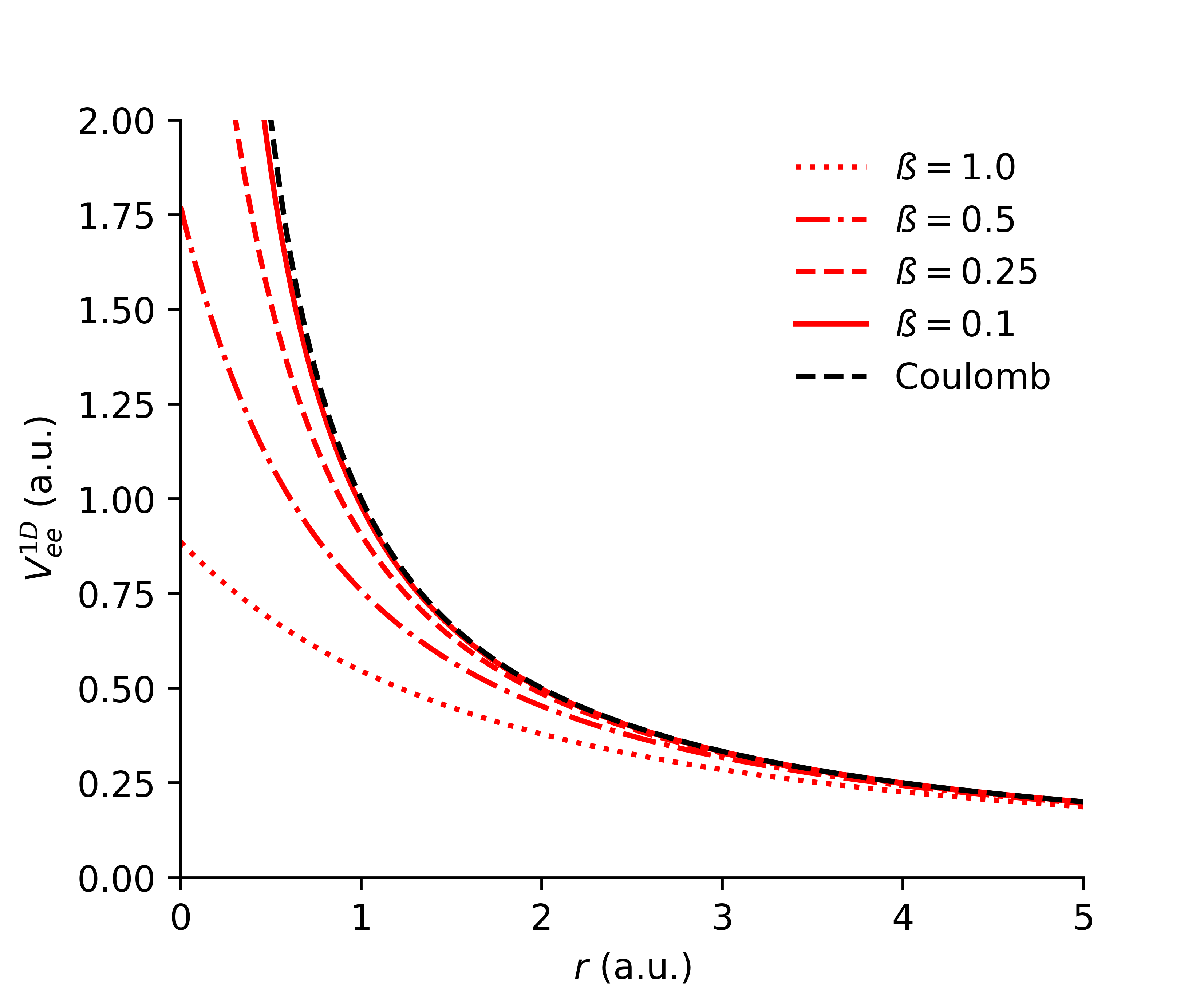
Proof.

For both (i) and (ii) we establish the conditions on the first and second moment of $v^{\prime\prime}$ as given in Assumption 1.

(i) Let $v$ be the convex soft Coulomb potential $\tilde{v}_{\varepsilon}$ . For the first moment we find

\displaystyle\int_{\gamma}^{\infty}v^{\prime\prime}r\mathrm{d}r\leq\frac{2}{((\gamma+r_{\varepsilon})^{2}+\varepsilon^{2})^{1/2}}\leq\frac{2}{\gamma}.

Furthermore note that $\int_{0}^{\gamma}v^{\prime\prime}r^{2}\mathrm{d}r\leq 2\int_{0}^{\gamma}v\mathrm{d}r$ such that

	$\displaystyle\int_{0}^{\gamma}v^{\prime\prime}r^{2}\mathrm{d}r$	$\displaystyle\leq 2\left[\ln(\sqrt{r^{2}+\varepsilon^{2}}+r)\right]_{r_{\varepsilon}}^{\gamma+r_{\varepsilon}}$
		$\displaystyle=2\ln\left(\frac{\gamma+r_{\varepsilon}}{r_{\varepsilon}}\frac{\sqrt{1+\varepsilon^{2}/(\gamma+r_{\varepsilon})^{2}}+1}{\sqrt{3}+1}\right)$
		$\displaystyle\leq 2\ln\left(\frac{\gamma+r_{\varepsilon}}{r_{\varepsilon}}\right)=2\ln\left(1+\frac{\gamma}{r_{\varepsilon}}\right).$

Thus Assumption 1 holds with the constants $c_{1}=c_{3}=2$ and $c_{2}=c_{2}(\varepsilon)=2/\varepsilon$ .

(ii) We now consider the case when $v$ is the regularized Coulomb potential $v_{\beta}$ . Integrating the second moment of $v^{\prime\prime}$ by parts, and using that $v^{\prime}(\gamma)\gamma^{2}-2\gamma v(\gamma)\leq 0$ yields

\int_{0}^{\gamma}v^{\prime\prime}(r)r^{2}\mathrm{d}r\leq 2\int_{0}^{\gamma}v(r)\mathrm{d}r.

Employing the upper bound in Eq. (20) we find

\displaystyle v(r)\leq\frac{2}{r+\sqrt{r^{2}+\frac{(4\beta^{2})}{\pi}}}

(23)

and therewith

\displaystyle\int_{0}^{\gamma}v^{\prime\prime}(r)r^{2}\mathrm{d}r\leq 4\ln\left(1+\frac{\sqrt{\pi}\gamma}{4\beta}\right).

For the other inequality, integrating the first moment of $v^{\prime\prime}$ by part yields

\int_{\gamma}^{\infty}v^{\prime\prime}(r)r\mathrm{d}r=-\gamma v^{\prime}(\gamma)+v(\gamma).

Using the lower bound in Eq. (20) we obtain

\displaystyle-\gamma v^{\prime}(\gamma)

\displaystyle\leq\frac{\gamma}{2\beta^{2}}\left(1-\frac{2}{1+\sqrt{1+\frac{8\beta^{2}}{\gamma^{2}}}}\right).

By the fact that $\sqrt{1+r}\leq 1+r/2$ for $r\geq 0$ , we find

\displaystyle 1-\frac{2}{1+\sqrt{1+\frac{8\beta^{2}}{\gamma^{2}}}}\leq\sqrt{1+\frac{8\beta^{2}}{\gamma^{2}}}-1\leq\frac{4\beta^{2}}{\gamma^{2}}.

Hence, $\int_{\gamma}^{\infty}v^{\prime\prime}(r)r\mathrm{d}r\leq 4/\gamma$ since $v(\gamma)\leq 2/\gamma$ by Eq. (23). To conclude, Assumption 1 is fulfilled with $c_{1}=c_{3}=4$ and $c_{2}=c_{2}(\beta)=\sqrt{\pi}/(4\beta)$ . ∎

Remark 6.

Note that $\mathrm{erfc}(r)\leq e^{-r^{2}}/(\sqrt{\pi}r)$ . This yields a tighter constant, $c_{3}=3$ , for the regularized Coulomb potential since it then follows that $v_{\beta}(\gamma)\leq 1/\gamma$ .

III.2 Conjectured bound in one dimension based on the scaling argument

The conjectured bound in Eq. (16) based on the universal scaling argument of Ref. 17 can be readily obtained for the contact potential. By simply inserting $v=\delta$ into the direct interaction energy $D(\rho_{\psi},\rho_{\psi})$ , we obtain

I_{\mathrm{xc}}(\psi)\geq-D(\rho_{\psi},\rho_{\psi})=-\frac{1}{2}\int_{\mathbb{R}}\rho_{\psi}^{2}\mathrm{d}x.

(24)

Note that Eq. (24) was proposed and motivated but the proof not spelled out in Ref. 17.

Furthermore, we can apply Lemma II.2 to (convex) approximate contact potentials (see Fig. 3). Let $\sigma>0$ and define

v_{\sigma}(r)=\left\{\begin{aligned} &\frac{2}{\sigma}-\frac{2r}{\sigma^{2}},&&0\leq r\leq\sigma,\\ &0,&&\sigma<r.\end{aligned}\right.

Since $\int_{\mathbb{R}}v_{\sigma}(r){\rm d}r=1$ , Eq. (9) with $\gamma>\sigma$ yields

I_{\mathrm{xc}}(\psi)\geq-\int_{\mathbb{R}}\rho_{\psi}^{2}\mathrm{d}x.

(Note that $\int_{\mathbb{R}}v_{\sigma}^{\prime\prime}r^{2}{\rm d}r=2$ can also be obtained using Eq. (10). In that case one either integrates by parts or insert the second order distributional derivative $v_{\sigma}(r)^{\prime\prime}=2\delta(r-\sigma)/\sigma^{2}$ .) This bound holds for all $\sigma>0$ . Note, however, that in the limit $\sigma\to 0+$ , we obtain a nonoptimal constant (twice as large as in Eq. (24)).

We next discuss the homogeneous potential $v(r)=r^{\varepsilon-1}$ . In this case Lemma II.1 with $\gamma=(\mathcal{M}\rho_{\psi})^{-1}$ gives a Lieb–Oxford bound that is arbitrarily close to the conjectured form in Eq. (16). (Di Marino has proven similar result in the setting of strictly correlated electrons Di Marino tbd.) This coincides with the general result of Lundholm et al., Lemma 16 in Ref. 34 with $d=1$ , viz.,

\displaystyle I_{\mathrm{xc}}(\psi)\geq-\frac{2^{2-\varepsilon}(2-\varepsilon)^{2}}{\varepsilon(1-\varepsilon)}\int_{\mathbb{R}}\rho_{\psi}^{2-\varepsilon}\mathrm{d}x.

(25)

As the conjectured form $\int_{\mathbb{R}}\rho_{\psi}^{2}\mathrm{d}x$ is approached, i.e., in the limit $\varepsilon\to 0_{+}$ , we have $2^{2-\varepsilon}(2-\varepsilon)^{2}/(\varepsilon(1-\varepsilon))\to+\infty$ , and where the use of the Hardy–Littlewood maximal function introduces the extra factor $2^{3-\varepsilon}(2-\varepsilon)/(1-\varepsilon)$ .

Alternatively, we here note that we can use Lemma II.2 to obtain the conjectured form for $v=r^{\varepsilon-1}$ and any $0<\varepsilon<1$ , although also with an unbounded constant as $\varepsilon\to 0+$ .

Theorem III.2.

Let $v(r)=r^{\varepsilon-1}$ and $0<\varepsilon<1$ , then

\displaystyle I_{\mathrm{xc}}(\psi)

\displaystyle\geq-\left(\frac{1}{\varepsilon}+\varepsilon-3\right)\int_{\mathbb{R}}\rho_{\psi}^{2}\mathrm{d}x-\left(1-\frac{\varepsilon}{2}\right)\int_{\mathbb{R}}\rho_{\psi}\mathrm{d}x.

In particular, there exists a $C_{\varepsilon}>0$ such that

\displaystyle I_{\mathrm{xc}}(\psi)\geq-C_{\varepsilon}\int_{\mathbb{R}}\rho_{\psi}^{2}\mathrm{d}x.

Proof.

Note that the homogeneous potential is convex and $\lim_{r\to\infty}v(r)=0$ . Hence, Lemma II.2 is applicable and the choice $\gamma=1$ gives

\displaystyle\frac{1}{2}\int_{{\mathbb{R}}}\rho_{\psi}^{2}\mathrm{d}x\int_{0}^{1}v^{\prime\prime}r^{2}\mathrm{d}r=\left(\frac{1}{\varepsilon}+\varepsilon-3\right)\int_{\mathbb{R}}\rho_{\psi}^{2}\mathrm{d}x,

and

\displaystyle\frac{1}{2}\int_{\mathbb{R}}\rho_{\psi}\mathrm{d}x\int_{1}^{\infty}v^{\prime\prime}r\mathrm{d}r

\displaystyle=\left(1-\frac{\varepsilon}{2}\right)\int_{\mathbb{R}}\rho_{\psi}\mathrm{d}x.

Since $\rho_{\psi}\in L^{1}(\mathbb{R})$ , we find for any $\varepsilon>0$ an interval $B_{\varepsilon}$ such that $\int_{\mathbb{R}}\rho_{\psi}\mathrm{d}x\leq\int_{B_{\varepsilon}}\rho_{\psi}\mathrm{d}x+N\varepsilon/2$ . Since $N\geq 2$ , we have

\left(1-\frac{\varepsilon}{2}\right)\int_{\mathbb{R}}\rho_{\psi}\mathrm{d}x>1

and

\left(1-\frac{\varepsilon}{2}\right)\int_{\mathbb{R}}\rho_{\psi}\mathrm{d}x\leq\left(\int_{B_{\varepsilon}}\rho_{\psi}\mathrm{d}x\right)^{2}\leq|B_{\varepsilon}|\int_{\mathbb{R}}\rho_{\psi}^{2}\mathrm{d}x.

Defining $C_{\epsilon}=|B_{\varepsilon}|+(\epsilon-3+1/\epsilon)$ concludes the proof. ∎

Remark 7.

As is evident from the proof, the conjectured bound for the case $v=r^{\varepsilon-1}$ is not the optimal formulation since for large particle number $\int_{\mathbb{R}}\rho_{\psi}\mathrm{d}x$ is significantly less than $\left(\int_{\mathbb{R}}\rho_{\psi}\mathrm{d}x\right)^{2}$ .

We finalize by commenting on the result in the previous section. The Lieb–Oxford bounds established for the convex soft Coulomb potential ( $\tilde{v}_{\varepsilon}$ ) and regularized Coulomb potential ( $v_{\beta}$ ) are not of the conjectured form $I_{\mathrm{xc}}(\psi)\geq-C_{1}\int_{\mathbb{R}}\rho_{\psi}^{2}\mathrm{d}x$ . However, using that $\ln(1+x)\leq x$ for $x\geq 0$ , Theorem III.1 yields with $\alpha=cN/(c_{1}c_{2})>0$

\displaystyle I_{\mathrm{xc}}(\psi)

\displaystyle\geq-\frac{c_{1}c_{2}c_{3}}{2c}\int_{\mathbb{R}}\rho_{\psi}^{2}\mathrm{d}x-\frac{1}{2}cN.

(26)

For the regularized Coulomb potential, where we can take $c_{1}=c_{3}=4$ and $c_{2}(\beta)=\sqrt{\pi}/(4\beta)$ , we have

\displaystyle I_{\mathrm{xc}}(\psi)+\frac{1}{2}cN

\displaystyle\geq-\frac{2\sqrt{\pi}}{c\beta}\int_{\mathbb{R}}\rho_{\psi}^{2}\mathrm{d}x,

(27)

and similarly for the convex soft Coulomb potential

\displaystyle I_{\mathrm{xc}}(\psi)+\frac{1}{2}cN

\displaystyle\geq-\frac{2\sqrt{2}}{c\varepsilon}\int_{\mathbb{R}}\rho_{\psi}^{2}\mathrm{d}x.

(28)

Generally, if the interaction potential is shifted down with a positive constant $v\to v^{\prime}=v-c$ , then the shifted interaction energy, $I_{\mathrm{xc}}^{\prime}$ , by definition satisfies $I_{\mathrm{xc}}^{\prime}=I_{\mathrm{xc}}+cN/2$ . In particular, for the regularized Coulomb potential the choice $c=v_{\beta}(0)=\sqrt{\pi}/(2\beta)=:c_{\beta}$ gives $I_{\mathrm{xc}}^{\prime}(\psi)\geq-4\int_{\mathbb{R}}\rho_{\psi}^{2}\mathrm{d}x$ , although the indirect interaction energy $I_{\mathrm{xc}}^{\prime}$ does not come from a repulsive potential anymore since $v_{\beta}^{\prime}:=v_{\beta}-c_{\beta}\leq 0$ .

IV Conclusion

In this article, we have discussed and presented one-dimensional Lieb–Oxford-type inequalities for different Coulomb-like potentials. Due to the strong singular nature of the Coulomb potential in one dimension, different choices of pseudopotentials have been employed and investigated. Although we were able to derive Lieb–Oxford bounds for a variety of Coulomb-like potentials, we have not found a general or parameter-independent bound. (The contact potential gives the constant $1/2$ but is not reproduced using the other potentials.) Our strategy follows the general framework of Hainzl and Seringer Hainzl and Seiringer 2001, although an alternative approach (see Lemma II.2) that does not use the Hardy–Littlewood maximal function has been established and subsequently used. We have focused on potentials that approximate the Coulomb potential and that have been previously addressed in the literature. In particular, Räsänen and coauthors Räsänen et al. 2009; Räsänen, Seidl, and Gori-Giorgi 2011 have studied Lieb–Oxford bounds for different interaction potentials. Reference 17 conjectured that the Lieb–Oxford bound for a one-dimensional system takes the form $I_{\mathrm{xc}}(\psi)\geq-C_{1}\int_{\mathbb{R}}\rho_{\psi}^{2}\mathrm{d}x$ . For the contact potential this can be directly established. We proved modified results for the soft and the regularized Coulomb potentials (see Section III.1) that also involve logarithmic terms of the particle density. For the regularized Coulomb potential, the proven Lieb–Oxford inequality in Theorem III.1 is, to the best of our knowledge, the first known explicit bound for this type of interaction. In Section III.2, we additionally investigated to what degree the conjectured bound could be established for approximate contact potentials, homogeneous potentials, soft Coulomb and regularized Coulomb potentials. This typically involves unbounded (Lieb–Oxford) constants. In particular, by applying Lemma II.2 we derived a Lieb–Oxford bound for the homogeneous potential $v=r^{\varepsilon-1}$ of the conjectured form but with unbounded constant (as $\varepsilon\to 0+$ ). Using the same lemma, similar results are discussed for (convex) soft and regularized Coulomb potentials.

Data Availability

Data sharing is not applicable to this article as no new data were created or analyzed in this study.

Appendix A Lieb–Oxford bound for the one-dimensional Hubbard model

The Hubbard model is used describe the transition between conducting and insulating systems Hubbard 1963; Altland and Simons 2010; Herring 1966. In the one-dimensional case, this can be identified by Hydrogen chains Essler et al. 2005. It is interesting to note that an expression similar to the conjectured bound in Eq. (4) (for the Schrödinger model) can be derived for the homogeneous one-dimensional Hubbard model. The theoretical framework described in Ref. 25 provides the necessary foundation for the following derivation.

We recall that the Hubbard Hamiltonian in second quantization is

	$\displaystyle\hat{H}$	$\displaystyle=-t\sum_{\sigma\in\{\uparrow,\downarrow\}}\sum_{i=1}^{L}\left(c_{i,\sigma}^{\dagger}c_{i+1,\sigma}+c_{i+1,\sigma}^{\dagger}c_{i,\sigma}\right)$
		$\displaystyle+U\sum_{i=1}^{L}c_{i\uparrow}^{\dagger}c_{i\uparrow}c_{i\downarrow}^{\dagger}c_{i\downarrow},$

where $L>0$ is the number of lattice sites, $t>0$ is the hopping integral and $U\geq 0$ is the strength of the on-site interaction that represents the electron repulsion. In order to describe the exchange-correlation energy, we use an interpolation formula for the ground-state energy of the homogeneous Hubbard model based on the Bethe ansatz Lieb and Wu 1994 (see e.g. Ref. 25 for more details).

Considering two different cases for the band filling, i.e., a less than half-filled electronic band ( $n=N/L\leq 1$ ) and a more than half-filled band ( $1<n=N/L\leq 2$ ), the energy expression reads Capelle et al. 2003

e(n,t,U)=\left\{\begin{aligned} -&\frac{2t\beta(U/t)}{\pi}\,\sin\left(\frac{\pi}{\beta(U/t)}n\right),&&0\leq n\leq 1,\\ &e(2-n,t,U)+U(n-1),&&1<n\leq 2,\end{aligned}\right.

where $n=N/L$ describes the band filling and $\beta\in[1,2]$ is a function of the ratio $U/t$ . The exchange-correlation energy is then given by

e_{\rm xc}(n,t,U)=e(n,t,U)-e(n,t,0)-e_{\rm H}(n,U),

(29)

where $e_{\rm H}$ is the Hartree energy, i.e., $e_{\rm H}(n,U)=Un^{2}/4$ . Note that $e(n,t,0)$ describes the noninteracting kinetic energy.

Proposition A.1.

Let $t>0$ and $U\geq 0$ be fixed but arbitrary. Then $E_{\mathrm{ex}}^{\mathrm{1DHM}}(n,t,U)\geq-\frac{U}{4}\sum_{i}n_{i}^{2}$ .

Proof.

We will first demonstrate that $e(n,t,U)-e(n,t,0)\geq 0$ . Let $0\leq n\leq 1$ , then

		$\displaystyle e(n,t,U)-e(n,t,0)$
		$\displaystyle\quad=\frac{2t}{\pi}\left[2\sin\left(\frac{\pi n}{2}\right)-\beta(U/t)\sin\left(\frac{\pi n}{\beta(U/t)}\right)\right]$
		$\displaystyle\quad=:\frac{2t}{\pi}f_{n}(\kappa),$

where $\kappa=\beta(U/t)$ . We claim that $f_{n}(\kappa)$ is a positive function on the interval $[1,2]$ , see Fig. 4. To show this, we just have to note that $f_{n}^{\prime}(\kappa)\leq 0$ for $\kappa\in[1,2]$ (using e.g. that $x\leq\tan(x)$ on $[0,\pi/2]$ and that the reverse inequality holds on $[\pi/2,\pi]$ ) and that (by sine angle addition identity)

	$\displaystyle f_{n}(1)$	$\displaystyle=\sin\left(\frac{\pi n}{2}\right)-\sin\left(\pi n\right)$
		$\displaystyle=\sin\left(\frac{\pi n}{2}\right)-2\cos\left(\frac{\pi n}{2}\right)\sin\left(\frac{\pi n}{2}\right)\geq 0=f_{n}(2).$

For $n>1$ (but less or equal to two), we repeat the above but with $m=2-n$ instead of $n$ . To complete the proof, we use Eq. (29) and that $f_{n}\geq 0$ such that

	$\displaystyle E_{\rm xc}^{\mathrm{1DHM}}(n,t,U)$	$\displaystyle=\sum_{i=1}^{L}\left(\frac{2t}{\pi}f_{n_{i}}(\kappa)-e_{\rm H}(n_{i},U)\right)$
		$\displaystyle\geq-\frac{U}{4}\sum_{i}n_{i}^{2}.$

∎

We note that in case of the homogeneous Hubbard model the lower bound of the indirect interaction energy in terms of the single-particle density takes a discrete form characterized by the site-occupation number $n_{i}$ , i.e., the expectation value of $c_{i\uparrow}^{\dagger}c_{i\uparrow}+c_{i\downarrow}^{\dagger}c_{i\downarrow}$ .

References

Kohn and Sham (1965) W. Kohn and L. J. Sham, “Self-consistent equations including exchange and correlation effects,” Physical review 140, A1133 (1965).
Perdew and Burke (1996) J. P. Perdew and K. Burke, “Comparison shopping for a gradient-corrected density functional,” Int. J. Quantum Chem. 57, 309–319 (1996).
Lieb (1979) E. H. Lieb, “A lower bound for coulomb energies,” Physics Letters A 70, 444 – 446 (1979).
Lieb and Oxford (1981) E. H. Lieb and S. Oxford, “Improved lower bound on the indirect coulomb energy,” Int. J. Quantum Chem. 19, 427–439 (1981).
Perdew, Burke, and Ernzerhof (1996) J. P. Perdew, K. Burke, and M. Ernzerhof, “Generalized gradient approximation made simple,” Phys. Rev. Lett. 77, 3865 (1996).
Perdew, Burke, and Ernzerhof (1997) J. P. Perdew, K. Burke, and M. Ernzerhof, “Generalized gradient approximation made simple [phys. rev. lett. 77, 3865 (1996)],” Phys. Rev. Lett. 78, 1396–1396 (1997).
Perdew et al. (2004) J. P. Perdew, J. Tao, V. N. Staroverov, and G. E. Scuseria, “Meta-generalized gradient approximation: Explanation of a realistic nonempirical density functional,” J. Chem. Phys. 120, 6898–6911 (2004).
Levy and Perdew (1993) M. Levy and J. P. Perdew, “Tight bound and convexity constraint on the exchange-correlation-energy functional in the low-density limit, and other formal tests of generalized-gradient approximations,” Phys. Rev. B 48, 11638–11645 (1993).
Odashima and Capelle (2009) M. M. Odashima and K. Capelle, “Nonempirical hyper-generalized-gradient functionals constructed from the lieb-oxford bound,” Phys. Rev. A 79, 062515 (2009).
Haunschild et al. (2012) R. Haunschild, M. M. Odashima, G. E. Scuseria, J. P. Perdew, and K. Capelle, “Hyper-generalized-gradient functionals constructed from the lieb-oxford bound: Implementation via local hybrids and thermochemical assessment,” J. Chem. Phys. 136, 184102 (2012).
Odashima and Capelle (2007) M. M. Odashima and K. Capelle, “How tight is the lieb-oxford bound?” J. Chem. Phys. 127, 054106 (2007).
Vela, Medel, and Trickey (2009) A. Vela, V. Medel, and S. Trickey, “Variable lieb–oxford bound satisfaction in a generalized gradient exchange-correlation functional,” J. Chem. Phys. 130, 244103 (2009).
Kin-Lic Chan and Handy (1999) G. Kin-Lic Chan and N. C. Handy, “Optimized lieb-oxford bound for the exchange-correlation energy,” Phys. Rev. A 59, 3075–3077 (1999).
Cotar and Petrache (2019) C. Cotar and M. Petrache, “Equality of the jellium and uniform electron gas next-order asymptotic terms for coulomb and riesz potentials,” arXiv:1707.07664v5 (2019).
Lewin, Lieb, and Seiringer (2019) M. Lewin, E. H. Lieb, and R. Seiringer, “Floating wigner crystal with no boundary charge fluctuations,” Phys. Rev. B 100, 035127 (2019).
Lieb, Solovej, and Yngvason (1995) E. H. Lieb, J. P. Solovej, and J. Yngvason, “Ground states of large quantum dots in magnetic fields,” Phys. Rev. B 51, 10646–10665 (1995).
Räsänen et al. (2009) E. Räsänen, S. Pittalis, K. Capelle, and C. R. Proetto, “Lower bounds on the exchange-correlation energy in reduced dimensions,” Phys. Rev. Lett. 102, 206406 (2009).
Benguria, Bley, and Loss (2012) R. D. Benguria, G. A. Bley, and M. Loss, “A new estimate on the indirect coulomb energy,” Int. J. Quantum Chem. 112, 1579–1584 (2012).
Benguria and Tušek (2012) R. D. Benguria and M. Tušek, “Indirect coulomb energy for two-dimensional atoms,” J. Math. Phys. 53, 095213 (2012).
Benguria, Gallegos, and Tušek (2012) R. D. Benguria, P. Gallegos, and M. Tušek, “A new estimate on the two-dimensional indirect coulomb energy,” in Annales Henri Poincaré, Vol. 13 (Springer, 2012) pp. 1733–1744.
Lewin and Lieb (2015) M. Lewin and E. H. Lieb, “Improved lieb-oxford exchange-correlation inequality with a gradient correction,” Phys. Rev. A 91, 022507 (2015).
Räsänen, Seidl, and Gori-Giorgi (2011) E. Räsänen, M. Seidl, and P. Gori-Giorgi, “Strictly correlated uniform electron droplets,” Phys. Rev. B 83, 195111 (2011).
Hainzl and Seiringer (2001) C. Hainzl and R. Seiringer, Lett. Math. Phys. 55, 133 (2001).
Fogler (2005) M. M. Fogler, “Ground-state energy of the electron liquid in ultrathin wires,” Phys. Rev. Lett. 94, 056405 (2005).
Capelle et al. (2003) K. Capelle, N. Lima, M. Silva, and L. Oliveira, “Density-functional theory for the hubbard model: numerical results for the luttinger liquid and the mott insulator,” in The fundamentals of electron density, density matrix and density functional theory in atoms, molecules and the solid state (Springer, 2003) pp. 145–168.
Lima et al. (2003) N. Lima, M. Silva, L. Oliveira, and K. Capelle, “Density functionals not based on the electron gas: Local-density approximation for a luttinger liquid,” Phys. Rev. Lett. 90, 146402 (2003).
Schönhammer, Gunnarsson, and Noack (1995) K. Schönhammer, O. Gunnarsson, and R. Noack, “Density-functional theory on a lattice: Comparison with exact numerical results for a model with strongly correlated electrons,” Phys. Rev. B 52, 2504 (1995).
Perdew et al. (2014) J. P. Perdew, A. Ruzsinszky, J. Sun, and K. Burke, “Gedanken densities and exact constraints in density functional theory,” J. Chem. Phys. 140, 18A533 (2014).
Lieb (1983) E. H. Lieb, “Density functionals for Coulomb-systems,” Int. J. Quantum Chem. 24, 243–277 (1983).
Lieb and Loss (2001) E. Lieb and M. Loss, Analysis (American Mathematical Society, 2001).
Odashima, Capelle, and Trickey (2009) M. M. Odashima, K. Capelle, and S. Trickey, “Tightened lieb- oxford bound for systems of fixed particle number,” J. Chem. Theory Comput. 5, 798–807 (2009).
Giuliani and Vignale (2005) G. Giuliani and G. Vignale, Quantum theory of the electron liquid (Cambridge university press, 2005).
Di Marino (tbd) S. Di Marino, “Work in preparation,” (tbd).
Lundholm, Nam, and Portmann (2016) D. Lundholm, P. T. Nam, and F. Portmann, “Fractional hardy–lieb–thirring and related inequalities for interacting systems,” Arch. Ration. Mech. Anal. 219, 1343–1382 (2016).
Hubbard (1963) J. Hubbard, “Electron correlations in narrow energy bands,” Proceedings of the Royal Society of London. Series A. Mathematical and Physical Sciences 276, 238–257 (1963).
Altland and Simons (2010) A. Altland and B. D. Simons, Condensed matter field theory (Cambridge university press, 2010).
Herring (1966) C. Herring, Magnetism, edited by G. Rado and H. Suhl, Vol. IV. (Academic Press, New York, 1966).
Essler et al. (2005) F. H. Essler, H. Frahm, F. Göhmann, A. Klümper, and V. E. Korepin, The one-dimensional Hubbard model (Cambridge University Press, 2005).
Lieb and Wu (1994) E. H. Lieb and F.-Y. Wu, “Absence of mott transition in an exact solution of the short-range, one-band model in one dimension,” in Exactly Solvable Models Of Strongly Correlated Electrons (World Scientific, 1994) pp. 9–12.