Classical and quantum controllability of a rotating symmetric molecule

Ugo Boscain Note: CNRS, Sorbonne Université, Inria, Université de Paris, Laboratoire Jacques-Louis Lions, Paris, France. (ugo.boscain@upmc.fr) Eugenio Pozzoli Note: Inria, Sorbonne Université, Université de Paris, CNRS, Laboratoire Jacques-Louis Lions, Paris, France(eugenio.pozzoli@inria.fr). Mario Sigalotti Note: Inria, Sorbonne Université, Université de Paris, CNRS, Laboratoire Jacques-Louis Lions, Paris, France (mario.sigalotti@inria.fr).

Abstract

In this paper we study the controllability problem for a symmetric-top molecule, both for its classical and quantum rotational dynamics. The molecule is controlled through three orthogonal electric fields interacting with its electric dipole. We characterize the controllability in terms of the dipole position: when it lies along the symmetry axis of the molecule neither the classical nor the quantum dynamics are controllable, due to the presence of a conserved quantity, the third component of the total angular momentum; when it lies in the orthogonal plane to the symmetry axis, a quantum symmetry arises, due to the superposition of symmetric states, which has no classical counterpart. If the dipole is neither along the symmetry axis nor orthogonal to it, controllability for the classical dynamics and approximate controllability for the quantum dynamics are proved to hold. The approximate controllability of the symmetric-top Schrödinger equation is established by using a Lie–Galerkin method, based on block-wise approximations of the infinite-dimensional systems.

Keywords: Quantum control, Schrödinger equation, rotational dynamics, symmetric-top molecule, bilinear control systems, Euler equation

1 Introduction

The control of molecular dynamics takes an important role in quantum physics and chemistry because of the variety of its applications, starting from well-established ones such as rotational state-selective excitation of chiral molecules ([15, 16]), and going further to applications in quantum information ([29]). For a general overview of controlled molecular dynamics one can see, for example, [22].

Rotations can, in general, couple to vibrations in the so-called ro-vibrational states. In our mathematical analysis, however, we shall restrict ourselves to the rotational states of the molecule. Due to its discrete quantization, molecular dynamics perfectly fits the mathematical quantum control theory which has been established until now. In fact, the control of the Schrödinger equation has attracted substantial interest in the last 15 years (see [3, 5, 9, 18, 21, 25] and references therein). Rigid molecules are subject to the classification of rigid rotors in terms of their inertia moments $I_{1}\leq I_{2}\leq I_{3}$ : one distinghuishes asymmetric-tops ( $I_{1}<I_{2}<I_{3}$ ), prolate symmetric-tops ( $I_{1}<I_{2}=I_{3}$ ), oblate symmetric-tops ( $I_{1}=I_{2}<I_{3}$ ), spherical-tops ( $I_{1}=I_{2}=I_{3}$ ), and linear-tops ( $I_{1}=0,\,I_{2}=I_{3}$ ).

The problem of controlling the rotational dynamics of a planar molecule by means of two orthogonal electric fields has been analyzed in [7], where approximate controllability has been proved using a suitable non-resonance property of the spectrum of the rotational Hamiltonian. In [8] the approximate controllability of a linear-top controlled by three orthogonal electric fields has been established. There, a new sufficient condition for controllability, called the Lie–Galerkin tracking condition, has been introduced in an abstract framework, and applied to the linear-top system.

Here, we study the symmetric-top (prolate, oblate, or spherical) as a generalization of the linear one, characterizing its controllability in terms of the position of its electric dipole moment. While for the linear-top two quantum numbers $j,m$ are needed to describe the motion, the main and more evident difference here is the presence of a third quantum number $k$ , which classically represents the projection of the total angular momentum on the symmetry axis of the molecule. This should not be a surprise, since the configuration space of a linear-top is the $2$ -sphere $S^{2}$ , while the symmetric-top evolves on the Lie group ${\rm SO}(3)$ , a three-dimensional manifold. As a matter of fact, by fixing $k=0$ , one recovers the linear-top as a subsystem inside the symmetric-top. It is worth mentioning that the general theory developed in [7, 13, 25] is based on non-resonance conditions on the spectrum of the internal Hamiltonian. A major difficulty in studying the controllability properties of the rotational dynamics is that, even in the case of the linear-top, the spectrum of the rotational Hamiltonian has severe degeneracies at the so-called $m$ -levels. The symmetric-top is even more degenerate, due to the additional presence of the so-called $k$ -levels.

The Schrödinger equation for a rotating molecule controlled by three orthogonal electric fields reads

\mathrm{i}\dfrac{\partial}{\partial t}\psi(R,t)=H\psi(R,t)+\sum_{l=1}^{3}u_{l}(t)B_{l}(R,\delta)\psi(R,t),\quad\psi(\cdot,t)\in L^{2}({\rm SO}(3)),

where $H=\frac{1}{2}\Big(\frac{P_{1}^{2}}{I_{1}}+\frac{P_{2}^{2}}{I_{2}}+\frac{P_{3}^{2}}{I_{3}}\Big)$ is the rotational Hamiltonian, $I_{1},I_{2},I_{3}$ are the moments of inertia of the molecule, $P_{1},P_{2},P_{3}$ are the angular momentum differential operators, and $B_{i}(R,\delta)=-\langle R\delta,e_{i}\rangle$ is the interaction Hamiltonian between the dipole moment $\delta$ of the molecule and the direction $e_{i}$ , $i=1,2,3$ . Finally, $R\in{\rm SO}(3)$ is the matrix which describes the configuration of the molecule in the space.

We shall study the symmetric-top, and set $I_{1}=I_{2}$ . Anyway, our analysis does not depend on whether $I_{3}\geq I_{2}$ or $I_{3}\leq I_{2}$ , so we are actually treating in this way both the cases of a prolate or oblate symmetric-top. The principal axis of inertia with associated inertia moment $I_{3}$ is then called symmetry axis of the molecule. The position of the electric dipole with respect to the symmetry axis plays a crucial role in our controllability analysis: a symmetric molecule with electric dipole collinear to the symmetry axis will be called genuine, otherwise it will be called accidental ([19, Section 2.6]). Most symmetric molecules present in nature are genuine. Nevertheless, it can happen that two moments of inertia of a real molecule are almost equal, by “accident”, although the molecule does not possess a $n$ -fold axis of symmetry with $n\geq 3$ ¹¹ 1 The existence of a $n$ -fold axis of symmetry (i.e., an axis such that a rotation of angle $2\pi/n$ about it leaves unchanged the distribution of atoms in the space) with $n\geq 3$ , implies that the top is genuine symmetric.For instance, the inertia moments of the chiral molecule HSOH are $I_{1}\sim I_{2}\ll I_{3}$ , while its dipole components are $\delta_{1}>\delta_{2}=\delta_{1}/2\gg\delta_{3}\neq 0$ ([27]). Such slightly asymmetric-tops are often studied in chemistry and physics in their symmetric-top approximations (see, e.g., [27],[19, Section 3.4]), which correspond in general to accidentally symmetric-tops. In this case, closed expression for the spectrum and the eigenfunctions of $H$ are known. The case of the asymmetric-top goes beyond the scope of this paper, but we remark that accidentally symmetric-tops may be used to obtain controllability of asymmetric-tops with a perturbative approach. The idea of studying the controllability of quantum systems in general configurations starting from symmetric cases (even if the latter have more degeneracies) has already been exploited, e.g., in [10, 23].

The position of the dipole moment turns out to play a decisive role: when it is neither along the symmetry axis, nor orthogonal to it, as in Figure 1 1, then approximate controllability holds, under some non-resonance conditions, as it is stated in Theorem 13. To prove it, we introduce in Theorem 10 a new controllability test for the multi-input Schrödinger equation, closely related to the Lie–Galerkin tracking condition. We then apply this result to the symmetric-top system. The control strategy is based on the excitation of the system with external fields in resonance with three families of frequencies, corresponding to internal spectral gaps. One frequency is used to overcome the $m$ -degeneracy in the spectrum, and this step is quite similar to the proof of the linear-top approximate controllability (Appendix A). The other two frequencies are used in a next step to break the $k$ -degeneracy, in a three-wave mixing scheme (Appendix B) typically used in quantum chemistry to obtain enantio- and state-selectivity for chiral molecules ([4, 17, 28]).

The two dipole configurations to which Theorem 13 does not apply are extremely relevant from the physical point of view. Indeed, the dipole moment of a symmetric-top lies usually along its symmetry axis (Figure 1 1), and if not, for accidentally symmetric-tops, it is often found in the orthogonal plane (Figure 1 1). Here two different symmetries arise, implying the non-controllability of these systems, as we prove, respectively, in Theorems 11 and 20. These two conserved quantities stimulated and motivated the study of the classical dynamics of the symmetric-top, presented in the first part of the paper: the first conserved quantity, appearing in Theorem 11, corresponds to a classical observable, that is, the component of the angular momentum along the symmetry axis, and it turns out to be a first integral also for the classical controlled dynamics, as remarked in Theorem 3. The second conserved quantity, appearing in Theorem 20, is more challenging, because it does not have a counterpart in the classical dynamics, being mainly due to the superposition of $k$ and $-k$ states in the quantum dynamics. We show that this position of the dipole still corresponds to a controllable system for the classical-top, while it does not for the quantum-top. Thus, the latter is an example of a system whose quantum dynamics are not controllable even though the classical dynamics are. The possible discrepancy between quantum and classical controllability has been already noticed, for example, in the harmonic oscillator dynamics ([24]). It should be noticed that the classical dynamics of a rigid body controlled with external torques (e.g., opposite pairs of gas jets) or internal torques (momentum exchange devices such as wheels) as studied in the literature (see, e.g., [2, Section 6.4], [6],[14], [20, Section 4.6]) differ from the ones considered here, where the controlled fields (i.e., the interaction between the electric field and the electric dipole) are not left-invariant and their action depends on the configuration of the rigid body in the space.

The paper is organized as follows: in Section 2 we study the controllability of the classical Hamilton equations for a symmetric-top. The main results are Theorems 3 and 4, where we prove, respectively, the non-controllability when the dipole lies along the symmetry axis of the body and the controllability in any other case. In Section 3 we study the controllability of the Schrödinger equation for a symmetric-top. The main controllability result is Theorem 13, where we prove the approximate controllability when the dipole is neither along the symmetry axis, nor orthogonal to it. In the two cases left, we prove the non-controllability in Theorems 11 and 20.

2 Classical symmetric-top molecule

2.1 Controllability of control-affine systems with recurrent drift

We recall in this section some useful results on the controllability properties of (finite-dimensional) control-affine systems.

Let $M$ be an $n$ -dimensional manifold, $X_{0},X_{1},\dots,X_{\ell}$ a family of smooth (i.e., $C^{\infty}$ ) vector fields on $M$ , $U\subset\mathbb{R}^{\ell}$ a set of control values which is a neighborhood of the origin. We consider the control system

\dot{q}=X_{0}(q)+\sum_{i=1}^{\ell}u_{i}(t)X_{i}(q),\qquad q\in M,

(1)

where the control functions $u$ are taken in $L^{\infty}(\mathbb{R},U)$ . The vector field $X_{0}$ is called the drift. The reachable set from $q_{0}\in M$ is

	$\displaystyle\mathrm{Reach}(q_{0}):=$	$\displaystyle\{q\in M\mid\exists\;u,T\text{ s.t. the solution to (\ref{control}) with }q(0)=q_{0}$
		$\displaystyle\text{ satisfies }q(T)=q\}.$

System (1) is said to be controllable if $\mathrm{Reach}(q_{0})=M$ for all $q_{0}\in M$ .

The family of vector fields $X_{0},X_{1},\dots,X_{\ell}$ is said to be Lie bracket generating if

\dim(\mathrm{Lie}_{q}\{X_{0},X_{1},\dots,X_{\ell}\})=n

for all $q\in M$ , where $\mathrm{Lie}_{q}\{X_{0},X_{1},\dots,X_{\ell}\}$ denotes the evaluation at $q$ of the Lie algebra generated by $X_{0},X_{1},\dots,X_{\ell}$ .

The following is a basic result in geometric control theory (see, for example, [20, Section 4.6]). Recall that a complete vector field $X$ on $M$ is said to be recurrent if for every open nonempty subset $V$ of $M$ and every time $t>0$ , there exists $\tilde{t}>t$ such that $\phi_{\tilde{t}}(V)\cap V\neq\emptyset$ , where $\phi_{\tilde{t}}$ denotes the flow of $X$ at time ${\tilde{t}}$ .

Theorem 1.

Let $U\subset\mathbb{R}^{m}$ be a neighborhood of the origin. If $X_{0}$ is recurrent and the family $X_{0},X_{1},\dots,X_{\ell}$ is Lie bracket generating, then system (1) is controllable.

A useful test to check that the Lie bracket generating condition holds true is given by the following simple lemma, whose proof is given for completeness.

Lemma 2.

If the family of analytic vector fields $X_{0},X_{1},\dots,X_{\ell}$ is Lie bracket generating on the complement of a subset $N\subset M$ and $\mathrm{Reach}(q)\not\subset N$ , for all $q\in N$ , then the family is Lie bracket generating on $M$ .

Proof.

Let $q\in N$ and $q_{1}\in\mathrm{Reach}(q)\setminus N$ . By the Orbit theorem applied to the case of analytic vector fields (see, e.g., [2, Chapter 5]) the dimension of $\mathrm{Lie}_{q}\{X_{0},X_{1},\dots,X_{\ell}\}$ and $\mathrm{Lie}_{q_{1}}\{X_{0},X_{1},\dots,X_{\ell}\}$ coincide. By assumption the latter is equal to $n$ , which implies that the same is true for the former. ∎

2.2 The classical dynamics of a molecule subject to electric fields

Since the translational motion (of the center of mass) of a rigid body is decoupled from the rotational motion, we shall assume that the molecule can only rotate around its center of mass. In detail, for any vector $v\in\mathbb{R}^{3}$ , denoting by $e_{1},e_{2},e_{3}$ a fixed orthonormal frame of $\mathbb{R}^{3}$ and by $a_{1},a_{2},a_{3}$ a moving orthonormal frame with the same orientation, both attached to the rigid body’s center of mass, the configuration of the molecule is identified with the unique $g\in{\rm SO}(3)$ such that $g\;(x,y,z)^{T}=(X,Y,Z)^{T}$ , where $(x,y,z)$ are the coordinates of $v$ with respect to $a_{1},a_{2},a_{3}$ , and $(X,Y,Z)$ are the coordinates of $v$ with respect to $e_{1},e_{2},e_{3}$ . In order to describe the equations on the tangent bundle ${\rm SO}(3)\times\mathfrak{so}(3)$ , we shall make use of the isomorphism of Lie algebras

A:(\mathbb{R}^{3},\times)\rightarrow(\mathfrak{so(3)},[\cdot,\cdot]),\quad P=\begin{pmatrix}P_{1}\\ P_{2}\\ P_{3}\end{pmatrix}\mapsto A(P)=\begin{pmatrix}0&-P_{3}&P_{2}\\ P_{3}&0&-P_{1}\\ -P_{2}&P_{1}&0\end{pmatrix}

where $\times$ is the vector product. As external forces to control the rotation of the molecule, we consider three orthogonal electric fields with intensities $u_{1}(t)$ , $u_{2}(t)$ , $u_{3}(t)$ and directions $e_{1},e_{2},e_{3}$ . We assume that

(u_{1},u_{2},u_{3})\in U\subset\mathbb{R}^{3},\quad(0,0,0)\in{\rm Interior}(U),

that is, the set $U\subset\mathbb{R}^{3}$ of admissible values for the triple $(u_{1},u_{2},u_{3})$ is a neighborhood of the origin. Denoting by $\delta$ the dipole of the molecule written in the moving frame, the three forces due to the interaction with the electric fields are $u_{i}(t)(g^{-1}(t)e_{i})\times\delta$ , $i=1,2,3.$ Then, the equations for the classical rotational dynamics of a molecule with inertia moments $I_{1},I_{2},I_{3}$ controlled with electric fields read

\begin{pmatrix}\dot{g}\\ \dot{P}\end{pmatrix}=X(g,P)+\sum_{i=1}^{3}u_{i}(t)Y_{i}(g,P),\quad(g,P)\in{\rm SO}(3)\times\mathbb{R}^{3},\ u\in U,

(2)

where

X(g,P):=\begin{pmatrix}gA(\beta P)\\ P\times(\beta P)\end{pmatrix},\quad Y_{i}(g,P):=\begin{pmatrix}0\\ (g^{-1}e_{i})\times\delta\end{pmatrix},\quad i=1,2,3,

(3)

and $P=(P_{1},P_{2},P_{3})^{T},\;\beta P=(P_{1}/I_{1},P_{2}/I_{2},P_{3}/I_{3})^{T}$ . Similarly to [20, Section 12.2] (where this is done for the heavy rigid body), these equations can be derived as Hamilton equations corresponding to the Hamiltonian

H=\frac{1}{2}\left(\frac{P_{1}^{2}}{I_{1}}+\frac{P_{2}^{2}}{I_{2}}+\frac{P_{3}^{2}}{I_{3}}\right)+V(g),\quad V(g)=-\sum_{i=1}^{3}u_{i}\langle(g^{-1}e_{i}),\delta\rangle

on ${\rm SO}(3)\times\mathbb{R}^{3}$ . System (2) can be seen as a control-affine system with $\ell=3$ controlled fields.

Rotating molecule dynamics can also be represented in terms of quaternions, lifting the dynamics from ${\rm SO}(3)$ to the $3$ -sphere $S^{3}$ , as follows. We denote by $\mathbb{H}$ the space of quaternions and we identify $S^{3}\subset\mathbb{R}^{4}$ with $\{q_{0}+\mathrm{i}q_{1}+\mathrm{j}q_{2}+\mathrm{k}q_{3}\in\mathbb{H}\mid q_{0}^{2}+q_{1}^{2}+q_{2}^{2}+q_{3}^{2}=1\}$ . We also identify $\mathbb{R}^{3}$ with $\{\mathrm{i}P_{1}+\mathrm{j}P_{2}+\mathrm{k}P_{3}\in\mathbb{H}\mid(P_{1},P_{2},P_{3})\in\mathbb{R}^{3}\}$ . Via this identification, the vector product $P\times\Omega$ becomes $\frac{1}{2}[P,\Omega]:=\frac{1}{2}(P\Omega-\Omega P)$ , for any $P,\Omega\in\mathbb{R}^{3}$ . Moreover, given $q=\cos(\alpha)+(q_{1},q_{2},q_{3})\sin(\alpha)\in S^{3}$ and $P\in\mathbb{R}^{3}$ , the quaternion product $qP\overline{q}$ is in $\mathbb{R}^{3}$ and corresponds to the rotation of $P$ of angle $2\alpha$ around the axis $(q_{1},q_{2},q_{3})$ . Hence, $S^{3}$ can be seen as a double covering space of ${\rm SO}(3)$ (see [1, Section 5.2] for further details). System (2) is lifted to $S^{3}\times\mathbb{R}^{3}$ to the system

\begin{cases}\begin{aligned} \dfrac{dq(t)}{dt}=&q(t)\beta P(t),\\ \dfrac{dP(t)}{dt}=&\frac{1}{2}[P(t),\beta P(t)]+\dfrac{u_{1}(t)}{2}[\overline{q(t)}\mathrm{i}q(t),\delta]+\frac{u_{2}(t)}{2}[\overline{q(t)}\mathrm{j}q(t),\delta]\\ &+\frac{u_{3}(t)}{2}[\overline{q(t)}\mathrm{k}q(t),\delta].\end{aligned}\end{cases}

(4)

We are going to use the quaternion representation in order to prove that the vector fields characterizing (4) form a Lie bracket generating family. As a consequence, the same will be true for (2).

2.3 Non-controllability of the classical genuine symmetric-top

In most cases of physical interest, the electric dipole $\delta$ of a symmetric-top molecule lies along the symmetry axis of the molecule. If $I_{1}=I_{2}$ , the symmetry axis is the third one, and we have that $\delta=(0,0,\delta_{3})^{T}$ , $\delta_{3}\neq 0$ , in the body frame. The corresponding molecule is called a genuine symmetric-top ([19, Section 2.6]).

Theorem 3.

The third angular momentum $P_{3}$ is a conserved quantity for the controlled motion (2) of the genuine symmetry-top molecule.

Proof.

In order to compute the equation satisfied by $P_{3}$ in (2), notice that

\displaystyle P(t)\times\beta P(t)=\begin{pmatrix}P_{1}(t)\\ P_{2}(t)\\ P_{3}(t)\end{pmatrix}\times\begin{pmatrix}P_{1}(t)/I_{2}\\ P_{2}(t)/I_{2}\\ P_{3}(t)/I_{3}\end{pmatrix}=\begin{pmatrix}\Big(\frac{1}{I_{3}}-\frac{1}{I_{2}}\Big)P_{2}(t)P_{3}(t)\\ \Big(\frac{1}{I_{2}}-\frac{1}{I_{3}}\Big)P_{1}(t)P_{3}(t)\\ 0\end{pmatrix}.

Moreover, $u_{i}(t)(g^{-1}(t)e_{i})\times\delta=u_{i}(t)(g^{-1}(t)e_{i})\times(0,0,\delta_{3})^{T}=(\star,\star,0)^{T}$ . Hence, for a genuine symmetric-top, the equation for $P_{3}$ becomes $\frac{dP_{3}(t)}{dt}=0$ . ∎

As a consequence, the controlled dynamics live in the hypersurfaces $\{P_{3}=\mathrm{const}\}$ and hence system (2) is not controllable in the $6$ -dimensional manifold ${\rm SO}(3)\times\mathbb{R}^{3}$ .

2.4 Controllability of the classical accidentally symmetric-top

In Theorem 3 we proved that $P_{3}$ is a first integral for equations (2), using both the symmetry of the mass and the symmetry of the charge, meaning that $I_{1}=I_{2}$ and $\delta=(0,0,\delta_{3})^{T}$ . We consider now a symmetric-top molecule with electric dipole $\delta$ not along the symmetry axis of the body, that is, $\delta=(\delta_{1},\delta_{2},\delta_{3})^{T}$ , with $\delta_{1}\neq 0$ or $\delta_{2}\neq 0$ . This system is usually called accidentally symmetric-top ([19, Section 2.6]).

Theorem 4.

For an accidentally symmetric-top molecule system (2) is controllable.

Proof.

The drift $X$ is recurrent, as observed in [2, Section 8.4]. Thus, by Theorem 1, to prove controllability it suffices to show that, for any $(g,P)\in{\rm SO}(3)\times\mathbb{R}^{3}$ , $\mathrm{dim}\Big(\mathrm{Lie}_{(g,P)}\{X,Y_{1},Y_{2},Y_{3}\}\Big)=6$ . Actually, we will find six vector fields in $\mathrm{Lie}\{X,Y_{1},Y_{2},Y_{3}\}$ whose span is six-dimensional everywhere but on a set of positive codimension, and we will conclude by applying Lemma 2. Notice that $[X,Y_{i}](g,P)=\begin{pmatrix}-gS(\beta[(g^{-1})e_{i}\times\delta])\\ \star\end{pmatrix}.$ Denote by $\Pi_{{\rm SO}(3)}$ the projection onto the ${\rm SO}(3)$ part of the tangent bundle, that is, $\Pi_{{\rm SO}(3)}:T({\rm SO}(3)\times\mathbb{R}^{3})\rightarrow T{\rm SO}(3).$ Then we have

	$\displaystyle\mathrm{span}$	$\displaystyle\{\Pi_{{\rm SO}(3)}X(g,P),\Pi_{{\rm SO}(3)}[X,Y_{1}](g,P),\Pi_{{\rm SO}(3)}[X,Y_{2}](g,P),\Pi_{{\rm SO}(3)}[X,Y_{3}](g,P)\}$
		$\displaystyle=gS\Big(\beta[\{\delta\}^{\perp}\oplus\mathrm{span}\{P\}]\Big).$

Hence, if $\langle P,\delta\rangle\neq 0$ , we have

	$\displaystyle\dim$	$\displaystyle\Big(\mathrm{span}\{\Pi_{{\rm SO}(3)}X(g,P),\Pi_{{\rm SO}(3)}[X,Y_{1}](g,P),\Pi_{{\rm SO}(3)}[X,Y_{2}](g,P),$
		$\displaystyle\Pi_{{\rm SO}(3)}[X,Y_{3}](g,P)\}\Big)=3.$		(5)

To go further in the analysis, it is convenient to use the quaternion parametrization (4) in which every field is polynomial. We have, in coordinates $q=(q_{0},q_{1},q_{2},q_{3})\in S^{3},P=(P_{1},P_{2},P_{3})\in\mathbb{R}^{3}$ ,

X(q,P)=\begin{pmatrix}q\beta P\\ \frac{1}{2}[P,\beta P]\end{pmatrix}=\begin{pmatrix}-q_{1}\frac{P_{1}}{I_{2}}-q_{2}\frac{P_{2}}{I_{2}}-q_{3}\frac{P_{3}}{I_{3}}\\[2.84526pt] q_{0}\frac{P_{1}}{I_{2}}+q_{2}\frac{P_{3}}{I_{3}}-q_{3}\frac{P_{2}}{I_{2}}\\[2.84526pt] q_{0}\frac{P_{2}}{I_{2}}-q_{1}\frac{P_{3}}{I_{3}}+q_{3}\frac{P_{1}}{I_{2}}\\[2.84526pt] q_{0}\frac{P_{3}}{I_{3}}+q_{1}\frac{P_{2}}{I_{2}}-q_{2}\frac{P_{1}}{I_{2}}\\[2.84526pt] \Big(\frac{1}{I_{3}}-\frac{1}{I_{2}}\Big)P_{2}P_{3}\\[2.84526pt] \Big(\frac{1}{I_{2}}-\frac{1}{I_{3}}\Big)P_{1}P_{3}\\[2.84526pt] 0\end{pmatrix},

Y_{1}(q,P)=\begin{pmatrix}0\\ \frac{1}{2}[\overline{q}\mathrm{i}q,\delta]\end{pmatrix}=\begin{pmatrix}0\\ 0\\ 0\\ 0\\ (q_{1}q_{2}-q_{0}q_{3})\delta_{3}-(q_{1}q_{3}+q_{0}q_{2})\delta_{2}\\ (q_{1}q_{3}+q_{0}q_{2})\delta_{1}-\frac{1}{2}(q_{0}^{2}+q_{1}^{2}-q_{2}^{2}-q_{3}^{2})\delta_{3}\\ \frac{1}{2}(q_{0}^{2}+q_{1}^{2}-q_{2}^{2}-q_{3}^{2})\delta_{2}-(q_{1}q_{2}-q_{0}q_{3})\delta_{1}\end{pmatrix},

Y_{2}(q,P)=\begin{pmatrix}0\\ \frac{1}{2}[\overline{q}\mathrm{j}q,\delta]\end{pmatrix}=\begin{pmatrix}0\\ 0\\ 0\\ 0\\ \frac{1}{2}(q_{0}^{2}-q_{1}^{2}+q_{2}^{2}-q_{3}^{2})\delta_{3}-(q_{2}q_{3}-q_{0}q_{1})\delta_{2}\\ (q_{2}q_{3}-q_{0}q_{1})\delta_{1}-(q_{1}q_{2}+q_{0}q_{3})\delta_{3}\\ (q_{1}q_{2}+q_{0}q_{3})\delta_{2}-\frac{1}{2}(q_{0}^{2}-q_{1}^{2}+q_{2}^{2}-q_{3}^{2})\delta_{1}\end{pmatrix}.

Let us consider the six vector fields $X,Y_{1},Y_{2},[X,Y_{1}],[X,Y_{2}],[[X,Y_{1}],Y_{1}]$ : we have that the determinant of the matrix obtained by removing the first row from the $7\times 6$ matrix

(X(q,P),Y_{1}(q,P),Y_{2}(q,P),[X,Y_{1}](q,P),[X,Y_{2}](q,P),[[X,Y_{1}],Y_{1}](q,P))

is equal to $S(q,P):=S_{1}(q)S_{2}(q)S_{3}(q)S_{4}(q)S_{5}(P)$ , where

		$\displaystyle S_{1}(q):=\frac{I_{2}-I_{3}}{{32}I_{2}^{{3}}I_{3}^{2}}q_{1},$
		$\displaystyle S_{2}(q):=(-2q_{1}q_{2}\delta_{1}+2q_{0}q_{3}\delta_{1}+q_{0}^{2}\delta_{2}+q_{1}^{2}\delta_{2}-(q_{2}^{2}+q_{3}^{2})\delta_{2}),$
		$\displaystyle S_{3}(q):=(q_{0}(-2q_{2}\delta_{1}+2q_{1}\delta_{2})+2q_{3}(q_{1}\delta_{1}+q_{2}\delta_{2})+(q_{0}^{2}-q_{1}^{2}-q_{2}^{2}+q_{3}^{2})\delta_{3})^{2},$
		$\displaystyle S_{4}(q):=(-2(q_{0}q_{2}+q_{1}q_{3})(\delta_{1}^{2}+\delta_{2}^{2})+((q_{0}^{2}+q_{1}^{2}-q_{2}^{2}-q_{3}^{2})\delta_{1}+2(q_{1}q_{2}-q_{0}q_{3})\delta_{2})\delta_{3}),$
		$\displaystyle S_{5}(P):=P_{1}\delta_{1}+P_{2}\delta_{2}+P_{3}\delta_{3}=\langle P,\delta\rangle.$

Hence, for all $(q,P)$ such that $S(q,P)\neq 0$ ,

	$\displaystyle\dim\Big(\mathrm{span}$	$\displaystyle\{X(q,P),Y_{1}(q,P),Y_{2}(q,P),[X,Y_{1}](q,P),[X,Y_{2}](q,P),$
		$\displaystyle[[X,Y_{1}],Y_{1}](q,P)\}\Big)=6,$

that is, outside the set $N:=\{(q,P)\in S^{3}\times\mathbb{R}^{3}\mid S(q,P)=0\}$ the family $X,Y_{1},Y_{2}$ is Lie bracket generating.

Now we are left to prove that $\mathrm{Reach}(q,P)\not\subset N$ for every $(q,P)\in N$ , and then to apply Lemma 2. Let us start by considering the factor $S_{5}$ of $S$ and notice that, for any fixed $q\in S^{3}$ , $\{S_{5}=0\}$ defines a surface inside $\{q\}\times\mathbb{R}^{3}$ . Denote by $\Pi_{\mathbb{R}^{3}}:T(S^{3}\times\mathbb{R}^{3})\to T\mathbb{R}^{3}$ the projection onto the $\mathbb{R}^{3}$ part of the tangent bundle. The vector field $\Pi_{\mathbb{R}^{3}}X$ is tangent to $\{S_{5}=0\}$ when

\langle\nabla_{P}S_{5},\Pi_{\mathbb{R}^{3}}X\rangle=\frac{1}{2}\langle\delta,[P,\beta P]\rangle=0,

that is, if and only if $P_{3}=0$ or $P_{2}\delta_{1}-P_{1}\delta_{2}=0$ . Notice that one vector between $\Pi_{\mathbb{R}^{3}}Y_{1},\Pi_{\mathbb{R}^{3}}Y_{2},\Pi_{\mathbb{R}^{3}}Y_{3}$ is not tangent to $\{P_{3}=0\}$ , otherwise

\mathrm{span}\{\Pi_{\mathbb{R}^{3}}Y_{1},\Pi_{\mathbb{R}^{3}}Y_{2},\Pi_{\mathbb{R}^{3}}Y_{3}\}\subset\{P_{3}=0\}=\begin{pmatrix}0\\ 0\\ 1\end{pmatrix}^{\perp}.

However, $\mathrm{span}\{\Pi_{\mathbb{R}^{3}}Y_{1},\Pi_{\mathbb{R}^{3}}Y_{2},\Pi_{\mathbb{R}^{3}}Y_{3}\}=\delta^{\perp},$ which would imply that $\delta$ is collinear to $(0,0,1)^{T}$ , which is impossible since the molecule is accidentally symmetric.

Concerning the hypersurface $\{P_{2}\delta_{1}-P_{1}\delta_{2}=0\}$ , we consider again $\Pi_{\mathbb{R}^{3}}X$ , which is tangent to it when $\langle\nabla_{P}(P_{2}\delta_{1}-P_{1}\delta_{2}),\Pi_{\mathbb{R}^{3}}X\rangle=0$ , that is, if and only if $P_{3}=0$ or $P_{1}\delta_{1}+P_{2}\delta_{2}=0$ . We treat the second case, being $P_{3}=0$ already treated. Hence, we consider the intersection

\begin{cases}P_{2}\delta_{1}-P_{1}\delta_{2}=0,&\\ P_{1}\delta_{1}+P_{2}\delta_{2}=0.&\end{cases}

The only solution of the system is $P_{1}=P_{2}=0$ , because the molecule is accidentally symmetric. Finally, when $P_{1}=P_{2}=0$ , we consider the two-dimensional distribution $\mathrm{span}\{\Pi_{\mathbb{R}^{3}}Y_{1},\Pi_{\mathbb{R}^{3}}Y_{2},\Pi_{\mathbb{R}^{3}}Y_{3}\}$ , which cannot be tangent to the $P_{3}$ axis.

Summarizing, if $\delta$ is not collinear to $(0,0,1)^{T}$ , we have

\mathrm{Reach}(q,P)\not\subset\{S_{5}=0\},\quad\forall(q,P)\in\{S_{5}=0\}.

To conclude, if $(q,P)\in\{S_{i}=0\}$ , $i=1,\dots,4$ , then we fix $P$ and we get two-dimensional strata $\{q\in S^{3}\mid S_{i}(q)=0\}\subset S^{3}$ . Now the projections of the vector fields $X,[X,Y_{1}],[X,Y_{2}],[X,Y_{3}]$ on the base part of the bundle span a three-dimensional vector space if $\langle P,\delta\rangle\neq 0$ , as observed in (5). So, by possibly steering $P$ to a point where $\langle P,\delta\rangle\neq 0$ , it is possible to exit from the union of $\{S_{i}=0\}$ . This concludes the proof of the theorem. ∎

2.5 Reachable sets of the classical genuine symmetric-top

Theorem 3 states that each hypersurface $\{P_{3}=\mathrm{const}\}$ is invariant for the controlled motion. Next we prove that the restriction of system (2) to any such hypersurface is controllable.

Theorem 5.

Let $I_{1}=I_{2}$ and $\delta=(0,0,\delta_{3})^{T}$ , $\delta_{3}\neq 0$ . Then for $({g}_{0},{P}_{0})\in{\rm SO}(3)\times\mathbb{R}^{3}$ , ${P}_{0}=(P_{01},P_{02},P_{03})$ , one has

\mathrm{Reach}(g_{0},P_{0})=\{(g,P)\in{\rm SO}(3)\times\mathbb{R}^{3}\mid P_{3}=P_{03}\}.

Proof.

From Theorem 3 we know that $\{P_{3}=\mathrm{const}\}$ is invariant. Since the drift $X$ is recurrent, it suffices to prove that system (2) is Lie bracket generating on the $5$ -dimensional manifold $\{P_{3}=\mathrm{const}\}$ .

We recall from (5) that, if $\langle P,\delta\rangle\neq 0$ , that is, if $P_{3}\neq 0$ , we have

	$\displaystyle\dim$	$\displaystyle\Big(\mathrm{span}\{\Pi_{{\rm SO}(3)}X(g,P),\Pi_{{\rm SO}(3)}[X,Y_{1}](g,P),\Pi_{{\rm SO}(3)}[X,Y_{2}](g,P),$
		$\displaystyle\Pi_{{\rm SO}(3)}[X,Y_{3}](g,P)\}\Big)=3.$

Moreover, since $\Pi_{\mathbb{R}^{3}}Y_{i}(q,P)=(g^{-1}e_{i})\times\delta$ for $i=1,2,3$ , we have that

\dim\Big(\mathrm{span}\{\Pi_{\mathbb{R}^{3}}Y_{1},\Pi_{\mathbb{R}^{3}}Y_{2},\Pi_{\mathbb{R}^{3}}Y_{3}\}\Big)=2

(6)

everywhere. Thus, if $P_{3}\neq 0$ , it follows that

	$\displaystyle\dim$	$\displaystyle\Big(\mathrm{span}\{X(g,P),Y_{1}(g,P),Y_{2}(g,P),Y_{3}(g,P),[X,Y_{1}](g,P),[X,Y_{2}](g,P),$
		$\displaystyle[X,Y_{3}](g,P)\}\Big)=5.$

So the system is Lie bracket generating on the manifold $\{P_{3}=\text{const}\neq 0\}$ .

We are left to consider the case $P_{3}=0$ . Notice that $\Pi_{\mathbb{R}^{3}}Y_{1},\Pi_{\mathbb{R}^{3}}Y_{2},\Pi_{\mathbb{R}^{3}}Y_{3}$ span a two-dimensional distribution for any value of $P_{3}$ . So we consider in the quaternion parametrization the projections of $X,[X,Y_{1}],[X,Y_{2}],[[X,Y_{1}],X]$ on the $S^{3}$ part of the bundle and we obtain

	$\displaystyle\dim$	$\displaystyle\Big(\mathrm{span}\{\Pi_{S^{3}}X(q,P),\Pi_{S^{3}}[X,Y_{1}](q,P),\Pi_{S^{3}}[X,Y_{2}](q,P),$
		$\displaystyle\Pi_{S^{3}}[[X,Y_{1}],X](q,P)\}\Big)=3,$

for $P_{3}=0$ , except when $q_{3}[2P_{2}(q_{1}q_{2}-q_{0}q_{3})+P_{1}(q_{0}^{2}+q_{1}^{2}-q_{2}^{2}-q_{3}^{2})]=0$ . This equation defines the union of two surfaces inside $S^{3}$ . (Notice that we can assume $P_{1}\neq 0$ and $P_{2}\neq 0$ because (6) gives local controllability in $(P_{1},P_{2})$ ). On $\{q_{3}=0\}$ , we have that $\Pi_{S^{3}}X$ is tangent if and only if $q_{1}P_{2}-q_{2}P_{1}=0$ . On the curve $\gamma\subset S^{3}$ of equation

\begin{cases}q_{3}=0,&\\ q_{1}P_{2}-q_{2}P_{1}=0,&\end{cases}

we can consider the two-dimensional distribution spanned by $\Pi_{S^{3}}[X,Y_{1}],\Pi_{S^{3}}[X,Y_{2}]$ , $\Pi_{S^{3}}[X,Y_{3}]$ , which is clearly not tangent to $\gamma$ . Following Lemma 2, the system is Lie bracket generating also on $\{q_{3}=0\}$ .

Analogously, on $\{2P_{2}(q_{1}q_{2}-q_{0}q_{3})+P_{1}(q_{0}^{2}+q_{1}^{2}-q_{2}^{2}-q_{3}^{2})=0\}$ we consider the vector field $\Pi_{S^{3}}[[[X,Y_{1}],X],Y_{2}]$ which is tangent if and only if $(q_{0}q_{2}+q_{1}q_{3})(P_{1}q_{0}q_{1}+P_{2}q_{0}q_{2}-P_{2}q_{1}q_{3}+P_{1}q_{2}q_{3})=0$ . Again, since the distribution spanned by $\Pi_{S^{3}}[X,Y_{1}],\Pi_{S^{3}}[X,Y_{2}]$ , $\Pi_{S^{3}}[X,Y_{3}]$ is two-dimensional, we can exit from the set of equations

\begin{cases}2P_{2}(q_{1}q_{2}-q_{0}q_{3})+P_{1}(q_{0}^{2}+q_{1}^{2}-q_{2}^{2}-q_{3}^{2})=0,&\\ (q_{0}q_{2}+q_{1}q_{3})(P_{1}q_{0}q_{1}+P_{2}q_{0}q_{2}-P_{2}q_{1}q_{3}+P_{1}q_{2}q_{3})=0,&\end{cases}

whose strata have dimension at most one. Thus, applying again Lemma 2, we can conclude that the restriction of the system to the manifold $\{P_{3}=0\}$ is Lie bracket generating. ∎

3 Quantum symmetric-top molecule

3.1 Controllability of the multi-input Schrödinger equation

Let $\ell\in\mathbb{N}$ and $U\subset\mathbb{R}^{\ell}$ be a neighborhood of the origin. Let $\mathcal{H}$ be an infinite-dimensional Hilbert space with scalar product $\langle\cdot,\cdot\rangle$ (linear in the first entry and conjugate linear in the second), $H,B_{1},\dots,B_{\ell}$ be (possibly unbounded) self-adjoint operators on $\mathcal{H}$ , with domains $D(H),D(B_{1}),\dots,D(B_{\ell})$ . We consider the controlled Schrödinger equation

\mathrm{i}\frac{d\psi(t)}{dt}=(H+\sum_{j=1}^{\ell}u_{j}(t)B_{j})\psi(t),\quad\psi(t)\in\mathcal{H},\quad u(t)\in U.

(7)

Definition 6.

•

We say that the operator $H$ satisfies ( $\mathbb{A}1$ ) if it has discrete spectrum with infinitely many distinct eigenvalues (possibly degenerate).
Denote by $\mathcal{B}$ a Hilbert basis $(\phi_{k})_{k\in\mathbb{N}}$ of $\mathcal{H}$ made of eigenvectors of $H$ associated with the family of eigenvalues $(\lambda_{k})_{k\in\mathbb{N}}$ and let $\mathcal{L}$ be the set of finite linear combination of eigenstates, that is,

$\mathcal{L}=\mathrm{span}\{\phi_{k}\mid k\in\mathbb{N}\}.$
•

We say that $(H,B_{1},\dots,B_{\ell},\mathcal{B})$ satisfies ( $\mathbb{A}2$ ) if $\phi_{k}\in D(B_{j})$ for every $k\in\mathbb{N}$ , $j=1,\dots,\ell$ .
•

We say that $(H,B_{1},\dots,B_{\ell},\mathcal{B})$ satisfies ( $\mathbb{A}3$ ) if

$H+\sum_{j=1}^{\ell}u_{j}B_{j}:\mathcal{L}\rightarrow\mathcal{H}$

is essentially self-adjoint for every $u\in U$ .
•

We say that $(H,B_{1},\dots,B_{\ell},\mathcal{B})$ satisfies ( $\mathbb{A}$ ) if $H$ satisfies ( $\mathbb{A}1$ ) and
$(H,B_{1},\dots,B_{\ell},\mathcal{B})$ satisfies ( $\mathbb{A}2$ ) and ( $\mathbb{A}3$ ).

If $(H,B_{1},\dots,B_{\ell},\mathcal{B})$ satisfies ( $\mathbb{A}$ ) then, for every $(u_{1},\dots,u_{\ell})\in U$ , $H+\sum_{j=1}^{\ell}u_{j}B_{j}$ generates a one-parameter group $e^{-\mathrm{i}t(H+\sum_{j=1}^{\ell}u_{j}B_{j})}$ inside the group of unitary operators $U(\mathcal{H})$ . It is therefore possible to define the propagator $\Gamma_{T}^{u}$ at time $T$ of system (7) associated with a piecewise constant control law $u(\cdot)=(u_{1}(\cdot),\dots,u_{\ell}(\cdot))$ by composition of flows of the type $e^{-\mathrm{i}t(H+\sum_{j=1}^{\ell}u_{j}B_{j})}$ .

Definition 7.

Let $(H,B_{1},\dots,B_{\ell},\mathcal{B})$ satisfy ( $\mathbb{A}$ ).

•

Given $\psi_{0},\psi_{1}$ in the unit sphere $\mathcal{S}$ of $\mathcal{H}$ , we say that $\psi_{1}$ is reachable from $\psi_{0}$ if there exist a time $T>0$ and a piecewise constant control law $u:[0,T]\rightarrow U$ such that $\psi_{1}=\Gamma_{T}^{u}(\psi_{0})$ . We denote by $\mathrm{Reach}(\psi_{0})$ the set of reachable points from $\psi_{0}$ .
•

We say that (7) is approximately controllable if for every $\psi_{0}\in\mathcal{S}$ the set $\mathrm{Reach}(\psi_{0})$ is dense in $\mathcal{S}$ .

As a byproduct of the techniques used to prove approximate controllability of (7) for our problem, we will actually obtain a slightly stronger controllability property. For this reason, let us introduce the notion of module-tracker (m-tracker, for brevity) that is, a system for which any given curve can be tracked up to (relative) phases. The identification up to phases of elements of $\mathcal{H}$ in the basis $\mathcal{B}=(\phi_{k})_{k\in\mathbb{N}}$ can be accomplished by the projection

\mathcal{M}:\psi\mapsto\sum_{k\in\mathbb{N}}|\langle\phi_{k},\psi\rangle|\phi_{k}.

Definition 8.

Let $(H,B_{1},\dots,B_{\ell},\mathcal{B})$ satisfy ( $\mathbb{A}$ ). We say that system (7) is an m-tracker if, for every $r\in\mathbb{N}$ , $\psi_{1},\dots,\psi_{r}$ in $\mathcal{H}$ , $\widehat{\Gamma}:[0,T]\rightarrow U(\mathcal{H})$ continuous with $\widehat{\Gamma}_{0}=\mathrm{Id}_{\mathcal{H}}$ , and $\epsilon>0$ , there exists an invertible increasing continuous function $\tau:[0,T]\rightarrow[0,T_{\tau}]$ and a piecewise constant control $u:[0,T_{\tau}]\rightarrow U$ such that

\|\mathcal{M}(\widehat{\Gamma}_{t}\psi_{k})-\mathcal{M}(\Gamma_{\tau(t)}^{u}\psi_{k})\|<\epsilon,\qquad k=1,\dots,r,

for every $t\in[0,T_{\tau}]$ .

Remark 9.

We recall that if system (7) is an m-tracker, then it is also approximately controllable, as noticed in [8, Remark 2.9].

Following [8] and [11], we now introduce some objects that we later use to state a sufficient condition for a system to be an m-tracker. The proposed sufficient condition can be seen as a generalization of the main controllability result in [8]. The main difference is that here, instead of testing a sequence of finite-dimensional properties on an increasing sequence of linear subspaces of $\mathcal{H}$ , we test them on a sequence of overlapping finite-dimensional spaces, not necessarily ordered by inclusion. This allows the sufficient condition to be checked block-wise.

Let $\{I_{j}\mid j\in\mathbb{N}\}$ be a family of finite subsets of $\mathbb{N}$ such that $\cup_{j\in\mathbb{N}}I_{j}=\mathbb{N}$ . Denote by $n_{j}$ the cardinality of $I_{j}$ . Consider the subspaces

\mathcal{M}_{j}:=\mathrm{span}\{\phi_{n}\mid n\in I_{j}\}\subset\mathcal{H}

and their associated orthogonal projections

\Pi_{\mathcal{M}_{j}}:\mathcal{H}\ni\psi\mapsto\sum_{n\in I_{j}}\langle\phi_{n},\psi\rangle\phi_{n}\in\mathcal{H}.

Given a linear operator $Q$ on $\mathcal{H}$ we identify the linear operator $\Pi_{\mathcal{M}_{j}}Q\Pi_{\mathcal{M}_{j}}$ preserving $\mathcal{M}_{j}$ with its complex matrix representation with respect to the basis $(\phi_{n})_{n\in I_{j}}$ . The set $\Sigma_{j}=\{|\lambda_{l}-\lambda_{l^{\prime}}|\mid l,l^{\prime}\in I_{j}\}$ is then the collection of the spectral gaps of $\Pi_{\mathcal{M}_{j}}H\Pi_{\mathcal{M}_{j}}$ . We define $B_{i}^{(j)}:=\Pi_{\mathcal{M}_{j}}B_{i}\Pi_{\mathcal{M}_{j}}$ for every $i=1,\dots,\ell$ .

If the element $(B_{i})_{l,k}$ is different from zero, then a control $u_{i}$ oscillating at frequency $|\lambda_{l}-\lambda_{k}|$ induces a population transfer between the states $\phi_{l}$ and $\phi_{k}$ ([12]). The dynamics of such a population transfer depend on the other pairs of states $\phi_{l^{\prime}}$ , $\phi_{k^{\prime}}$ having the same spectral gap and whose corresponding element $(B_{i})_{l^{\prime},k^{\prime}}$ is different from zero. We are interested in controlling the induced population dynamics within a space ${\cal M}_{j}$ . This motivates the definition of the sets

	$\displaystyle\Xi_{j}^{0}=\{(\sigma,i)\in\Sigma_{j}\times\{1,\dots,\ell\}\mid\mbox{}$	$\displaystyle(B_{i})_{l,k}=0\ \mbox{for every }l\in\mathbb{N},\ k\in\mathbb{N}\setminus I_{j}$
		$\displaystyle\mbox{ such that }\|\lambda_{l}-\lambda_{k}\|=\sigma\},$

and

	$\displaystyle\Xi_{j}^{1}=\{(\sigma,i)\in\Sigma_{j}\times\{1,\dots,\ell\}\mid\mbox{}$	$\displaystyle(B_{i})_{l,k}=0\ \mbox{for every }l\in I_{j},\ k\in\mathbb{N}\setminus I_{j}$
		$\displaystyle\mbox{ such that }\|\lambda_{l}-\lambda_{k}\|=\sigma\}.$

While the set $\Xi_{j}^{1}$ compares only with pairs of states $\phi_{l},\phi_{k}$ with $\phi_{l}$ in ${\cal M}_{j}$ , such a requirement is not present in the definition if $\Xi_{j}^{0}$ . This means that for $(\sigma,i)\in\Xi_{j}^{0}$ the induced population dynamics obtained by a control $u_{i}$ oscillating at frequency $\sigma$ not only does not produce population transfer out of ${\cal M}_{j}$ , but also is trivial within the orthogonal complement to ${\cal M}_{j}$ .

For every $\sigma\geq 0$ , and every square matrix $M$ of dimension $m$ , let

\mathcal{E}_{\sigma}(M)=(M_{l,k}\delta_{\sigma,|\lambda_{l}-\lambda_{k}|})_{l,k=1,\dots,m},

where $\delta_{l,k}$ is the Kronecker delta. The $n_{j}\times n_{j}$ matrix $\mathcal{E}_{\sigma}(B_{i}^{(j)})$ corresponds to the activation in $B_{i}^{(j)}$ of the spectral gap $\sigma\in\Sigma_{j}$ : every element is $0$ except for the $(l,k)$ -elements such that $|\lambda_{l}-\lambda_{k}|=\sigma$ . A control $u_{i}$ oscillating at frequency $\sigma$ can induce the dynamics in ${\cal M}_{j}$ described by the matrix $\mathcal{E}_{\sigma}(B_{i}^{(j)})$ , and also, by phase modulation, those described by the matrix $W_{\xi}$ , $\xi\in S^{1}\subset\mathbb{C}$ , defined by

(W_{\xi}(M))_{l,k}=\begin{cases}\xi M_{l,k},&\lambda_{l}<\lambda_{k},\\ 0,&\lambda_{l}=\lambda_{k},\\ \bar{\xi}M_{l,k},&\lambda_{l}>\lambda_{k}.\end{cases}

(8)

Let us consider the sets of excited modes

\nu_{j}^{s}:=\{W_{\xi}(\mathcal{E}_{\sigma}(\mathrm{i}B_{i}^{(j)}))\mid(\sigma,i)\in\Xi_{j}^{s},\sigma\neq 0,\xi\in S^{1}\},\quad s=0,1.

(9)

Notice that $\nu_{j}^{0}\subset\nu_{j}^{1}\subset\mathfrak{su}(n_{j})$ . Indeed, we have the following picture:

\mathcal{E}_{\sigma}(\mathrm{i}B_{i}^{(j)})\in\nu_{j}^{0}\Rightarrow\mathcal{E}_{\sigma}(\Pi_{j-1,j,j+1}\mathrm{i}B_{i}\Pi_{j-1,j,j+1})=\left[\begin{array}[]{c|c|c}0&0&0\\ \hline\cr 0&\mathcal{E}_{\sigma}(\mathrm{i}B_{i}^{(j)})&0\\ \hline\cr 0&0&0\end{array}\right]

\mathcal{E}_{\sigma}(\mathrm{i}B_{i}^{(j)})\in\nu_{j}^{1}\Rightarrow\mathcal{E}_{\sigma}(\Pi_{j-1,j,j+1}\mathrm{i}B_{i}\Pi_{j-1,j,j+1})=\left[\begin{array}[]{c|c|c}*&0&*\\ \hline\cr 0&\mathcal{E}_{\sigma}(\mathrm{i}B_{i}^{(j)})&0\\ \hline\cr*&0&*\end{array}\right]

where $\Pi_{j-1,j,j+1}$ denotes the projection onto $\mathcal{M}_{j-1}\oplus\mathcal{M}_{j}\oplus\mathcal{M}_{j+1}$ .

We denote by $\mathrm{Lie}(\nu_{j}^{s})$ the Lie subalgebra of $\mathfrak{su}(n_{j})$ generated by the matrices in $\nu_{j}^{s}$ , $s=0,1$ , and define $\mathcal{T}_{j}$ as the minimal ideal of $\mathrm{Lie}(\nu_{j}^{1})$ containing $\nu_{j}^{0}$ .

Finally, we introduce the graph $\mathcal{G}$ with vertices $\mathcal{V}=\{I_{j}\mid j\in\mathbb{N}\}$ and edges $\mathcal{E}=\{(I_{j},I_{k})\mid j,k\in\mathbb{N},\;I_{j}\cap I_{k}\neq\emptyset\}$ . We are now in a position to state a new sufficient condition for a system to be an m-tracker, and thus, approximately controllable.

Theorem 10.

Assume that ( $\mathbb{A}$ ) holds true. If the graph $\mathcal{G}$ is connected and $\mathcal{T}_{j}=\mathfrak{su}(n_{j})$ for every $j\in\mathbb{N}$ , then (7) is an m-tracker.

Proof.

The proof works by applying Theorem 2.8 in [8], which guarantees that (7) is an m-tracker if a suitable condition, called Lie–Galerkin tracking condition ([8, Definition 2.7]), holds true. In terms of the notation introduced here, the Lie–Galerkin tracking condition is true if there exists a sequence $\{\widetilde{I}_{j}\mid j\in\mathbb{N}\}$ of finite subsets of $\mathbb{N}$ , strictly increasing with respect to the inclusion, such that $\cup_{j\in\mathbb{N}}\widetilde{I}_{j}=\mathbb{N}$ and $\mathcal{T}_{j}=\mathfrak{su}(n_{j})$ for every $j\in\mathbb{N}$ .

Up to reordering the sets $I_{j}$ , we can assume that

I_{j+1}\cap(\cup_{k=1}^{j}I_{k})\not=\emptyset,\qquad\forall j\in\mathbb{N}.

(10)

For $j\in\mathbb{N}$ , let $\widetilde{I}_{j}=\cup_{i=1}^{j}I_{i}$ and ${\cal Z}_{j}=\sum_{k=1}^{j}\mathcal{M}_{k}.$

The Lie–Galerkin tracking condition holds true if

\mathrm{Lie}(\cup_{j=1}^{m}\widetilde{\mathcal{T}}_{j})=\mathfrak{su}(\dim({\cal Z}_{m})),\qquad m\in\mathbb{N},

(11)

where the set of operators $\widetilde{\mathcal{T}}_{j}$ is obtained similarly to $\mathcal{T}_{j}$ , replacing $\nu_{j}^{s}$ , $s=0,1$ , by

\{W_{\xi}(\mathcal{E}_{\sigma}(\mathrm{i}\Pi_{{\cal Z}_{m}}B_{i}\Pi_{{\cal Z}_{m}}))\mid(\sigma,i)\in\Xi_{j}^{s},\sigma\neq 0,\xi\in S^{1}\},\quad s=0,1.

We proceed by induction on $m$ . For $m=1$ , (11) is true, since we have that $\mathrm{Lie}(\mathcal{T}_{1})=\mathcal{T}_{1}=\mathfrak{su}(n_{1})=\mathfrak{su}(\dim(\mathcal{Z}_{1}))$ . Assume now that (11) is true for $m$ , and consider the vertex $I_{m+1}\in{\cal V}$ . Consider $t,p\in\cup_{j=1}^{m+1}I_{j}$ and let us prove that $G_{t,p}:=e_{t,p}-e_{p,t}$ is in $\mathrm{Lie}(\cup_{j=1}^{m+1}\widetilde{\mathcal{T}}_{j})$ , where $e_{a,b}$ is the matrix with all entries equal to 0 except for the one in row $a$ and column $b$ , which is equal to 1 (and the indices in $\cup_{j=1}^{m+1}I_{j}$ are identified with the elements of $\{1,\dots,\dim({\cal Z}_{m+1})\}$ ). Decomposing ${\cal Z}_{m+1}$ as a direct orthogonal sum $V_{1}\oplus({\cal Z}_{m}\cap{\cal M}_{m+1})\oplus V_{2}$ with $V_{1}\subset{\cal Z}_{m}$ and $V_{2}\subset{\cal M}_{m+1}$ , a matrix in $\widetilde{\mathcal{T}}_{m+1}$ has the form

\left[\begin{array}[]{c|c|c}0&0&0\\ \hline\cr 0&Q_{11}&Q_{12}\\ \hline\cr 0&Q_{21}&Q_{22}\end{array}\right],\qquad\left[\begin{array}[]{c|c}Q_{11}&Q_{12}\\ \hline\cr Q_{21}&Q_{22}\end{array}\right]\in\mathfrak{su}(n_{m+1}),

as it follows from the definition of $\Xi_{j}^{0}$ and $\Xi_{j}^{1}$ and the fact that $\widetilde{\mathcal{T}}_{m+1}$ is the ideal generated by $\nu_{j}^{0}$ inside ${\rm Lie}(\nu_{j}^{1})$ . Similarly, a matrix in $\cup_{j=1}^{m}\widetilde{\mathcal{T}}_{j}$ has the form

\left[\begin{array}[]{c|c|c}Q_{11}&Q_{12}&0\\ \hline\cr Q_{21}&Q_{22}&0\\ \hline\cr 0&0&0\end{array}\right],\qquad\left[\begin{array}[]{c|c}Q_{11}&Q_{12}\\ \hline\cr Q_{21}&Q_{22}\end{array}\right]\in\mathfrak{su}(\dim({\cal Z}_{m})).

If $t,p\in\cup_{j=1}^{m}I_{j}$ or $t,p\in I_{m+1}$ the conclusion follows from the induction hypothesis and the identity $\mathcal{T}_{m+1}=\mathfrak{su}(n_{m+1})$ . Let then $t\in I_{m+1}\setminus(\cup_{j=1}^{m}I_{j})$ and $p\in\cup_{j=1}^{m}I_{j}$ . Fix, moreover, $r\in I_{m+1}\cap(\cup_{j=1}^{m}I_{j})$ , whose existence is guaranteed by (10). Again by the induction hypothesis and the identity $\mathcal{T}_{m+1}=\mathfrak{su}(n_{m+1})$ , we have that $G_{p,r}$ and $G_{r,t}$ are in $\mathrm{Lie}(\cup_{j=1}^{m+1}\widetilde{\mathcal{T}}_{j})$ . The bracket $[G_{p,r},G_{r,t}]=G_{p,t}$ is therefore also in $\mathrm{Lie}(\cup_{j=1}^{m+1}\widetilde{\mathcal{T}}_{j})$ . By similar arguments, we deduce that every element of a basis of $\mathfrak{su}(\dim({\cal Z}_{m+1}))$ is in $\mathrm{Lie}(\cup_{j=1}^{m+1}\widetilde{\mathcal{T}}_{j})$ . ∎

3.2 The Schrödinger equation of a symmetric-top subject to electric fields

We recall in this section some general facts about Wigner functions and the theory of angular momentum in quantum mechanics (see, for instance, [26, 19]).

We use Euler’s angles $(\alpha,\beta,\gamma)\in[0,2\pi)\times[0,\pi]\times[0,2\pi)$ to describe the configuration space ${\rm SO}(3)$ of the molecule. More precisely, the coordinates of a vector change from the body fixed frame $a_{1},a_{2},a_{3}$ to the space fixed frame $e_{1},e_{2},e_{3}$ via three rotations

\begin{pmatrix}X\\ Y\\ Z\end{pmatrix}=R_{e_{3}}(\alpha)R_{e_{2}}(\beta)R_{e_{3}}(\gamma)\begin{pmatrix}x\\ y\\ z\end{pmatrix}=:R(\alpha,\beta,\gamma)\begin{pmatrix}x\\ y\\ z\end{pmatrix}

(12)

where $(x,y,z)^{T}$ are the coordinates of the vector in the body fixed frame, $(X,Y,Z)^{T}$ are the coordinates of the vector in the space fixed frame and $R_{e_{i}}(\theta)\in{\rm SO}(3)$ is the rotation of angle $\theta$ around the axis $e_{i}$ . The explicit expression of the matrix $R(\alpha,\beta,\gamma)\in{\rm SO}(3)$ is

R=\begin{pmatrix}\cos\alpha\cos\beta\cos\gamma-\sin\alpha\sin\gamma&-\cos\alpha\cos\beta\sin\gamma-\sin\alpha\cos\gamma&\cos\alpha\sin\beta\\ \sin\alpha\cos\beta\cos\gamma+\cos\alpha\sin\gamma&-\sin\alpha\cos\beta\sin\gamma+\cos\alpha\cos\gamma&\sin\alpha\sin\beta\\ -\sin\beta\cos\gamma&\sin\beta\sin\gamma&\cos\beta\end{pmatrix}.

(13)

In Euler coordinates, the angular momentum operators are given by

\begin{cases}\begin{aligned} J_{1}&=\mathrm{i}\cos\alpha\cot\beta\dfrac{\partial}{\partial\alpha}+\mathrm{i}\sin\alpha\dfrac{\partial}{\partial\beta}-\mathrm{i}\dfrac{\cos\alpha}{\sin\beta}\dfrac{\partial}{\partial\gamma},\\ J_{2}&=\mathrm{i}\sin\alpha\cot\beta\dfrac{\partial}{\partial\alpha}-\mathrm{i}\cos\alpha\dfrac{\partial}{\partial\beta}-\mathrm{i}\dfrac{\sin\alpha}{\sin\beta}\dfrac{\partial}{\partial\gamma},\\ J_{3}&=-\mathrm{i}\dfrac{\partial}{\partial\alpha}.\end{aligned}\end{cases}

(14)

These are linear operators acting on the Hilbert space $L^{2}({\rm SO}(3))$ , self-adjoint with respect to the Haar measure $\frac{1}{8}d\alpha d\gamma\sin\beta d\beta$ . Using (14), the self-adjoint operator $P_{3}:=-\mathrm{i}\frac{\partial}{\partial\gamma}$ can be written as $P_{3}=\sin\beta\cos\alpha J_{1}+\sin\beta\sin\alpha J_{2}+\cos\beta J_{3}$ , that is,

P_{3}=\sum_{i=1}^{3}R_{i3}(\alpha,\beta,\gamma)J_{i},

where $R=(R_{ij})_{i,j=1}^{3}$ is given in (13).

In the same way we define $P_{1}=\sum_{i=1}^{3}R_{i1}(\alpha,\beta,\gamma)J_{i},P_{2}=\sum_{i=1}^{3}R_{i2}(\alpha,\beta,\gamma)J_{i}$ . The operators $J_{i}$ and $P_{i}$ , $i=1,2,3$ , are the angular momentum operators expressed in the fixed and in the body frame, respectively. Finally, we consider the square norm operator $J^{2}:=J_{1}^{2}+J_{2}^{2}+J_{3}^{2}=P_{1}^{2}+P_{2}^{2}+P_{3}^{2}$ . Now, $J^{2},J_{3},P_{3}$ can be considered as the three commuting observables needed to describe the quantum motion of a molecule. Indeed, $[J^{2},J_{3}]=[J^{2},P_{3}]=[J_{3},P_{3}]=0$ , and hence there exists an orthonormal Hilbert basis of $L^{2}({\rm SO}(3))$ which diagonalizes simultaneously $J^{2},J_{3}$ and $P_{3}$ . In terms of Euler coordinates, this basis is made by the so-called Wigner functions

D_{k,m}^{j}(\alpha,\beta,\gamma):=e^{\mathrm{i}(m\alpha+k\gamma)}d_{k,m}^{j}(\beta),\qquad j\in\mathbb{N},\quad k,m=-j,\dots,j,

(15)

where the function $d^{j}_{k,m}$ solves a suitable Legendre differential equation, obtained by separation of variables (see, e.g., [19, Section 2.5] for the separation of variables ansatz and [26, Chapter 4] for a detailed description of the properties of these functions).

Summarizing, the family of Wigner functions $\{D_{k,m}^{j}\mid j\in\mathbb{N},k,m=-j,\dots,j\}$ forms an orthonormal Hilbert basis for $L^{2}({\rm SO}(3))$ . Moreover,

J^{2}D_{k,m}^{j}=j(j+1)D_{k,m}^{j},\quad J_{3}D_{k,m}^{j}=mD_{k,m}^{j},\quad P_{3}D_{k,m}^{j}=kD_{k,m}^{j}.

Thus, $m$ and $k$ are the quantum numbers which correspond to the projections of the angular momentum on the third axis of, respectively, the fixed and the body frame.

The rotational Hamiltonian of a molecule is $H=\frac{1}{2}\Big(\frac{P_{1}^{2}}{I_{1}}+\frac{P_{2}^{2}}{I_{2}}+\frac{P_{3}^{2}}{I_{3}}\Big)$ , which is seen here as a self-adjoint operator acting on the Hilbert space $L^{2}({\rm SO}(3))$ . From now on, we impose the symmetry relation $I_{1}=I_{2}$ , which implies that $H=\frac{J^{2}}{2I_{2}}+\Big(\frac{1}{2I_{3}}-\frac{1}{2I_{2}}\Big)P_{3}^{2}$ . Thus,

HD_{k,m}^{j}=\Big(\dfrac{j(j+1)}{2I_{2}}+\Big(\dfrac{1}{2I_{3}}-\dfrac{1}{2I_{2}}\Big)k^{2}\Big)D_{k,m}^{j}=:E_{k}^{j}D_{k,m}^{j}.

(16)

Hence, the Wigner functions are the eigenfunctions of $H$ . Since the eigenvalues of $H$ do not depend on $m$ , the energy level $E_{k}^{j}$ is $(2j+1)$ -degenerate with respect to $m$ . This property is common to every molecule in nature: the spectrum $\sigma(H)$ does not depend on $m$ , just like in classical mechanics kinetic energy does not depend on the direction of the angular momentum. Moreover, when $k\neq 0$ the energy level $E_{k}^{j}$ is also $2$ -degenerate with respect to $k$ . This extra degeneracy is actually a characterizing property of symmetric molecules. Breaking this $k$ -symmetry will be one important feature of our controllability analysis.

The interaction Hamiltonian between the dipole $\delta$ inside the molecule and the external electric field in the direction $e_{i}$ , $i=1,2,3$ , is given by the Stark effect ([19, Chapter 10])

B_{i}(\alpha,\beta,\gamma)=-\langle R(\alpha,\beta,\gamma)\delta,e_{i}\rangle,

seen as a multiplicative self-adjoint operator acting on $L^{2}({\rm SO}(3))$ . Thus, the rotational Schrödinger equation for a symmetric-top molecule subject to three orthogonal electric fields reads

\mathrm{i}\dfrac{\partial}{\partial t}\psi(\alpha,\beta,\gamma;t)=H\psi(\alpha,\beta,\gamma;t)+\sum_{l=1}^{3}u_{l}(t)B_{l}(\alpha,\beta,\gamma)\psi(\alpha,\beta,\gamma;t),

(17)

with $\psi(t)\in L^{2}({\rm SO}(3))$ and $u(t)\in U$ , for some neighborhood $U$ of $0$ in $\mathbb{R}^{3}$ .

3.3 Non-controllability of the quantum genuine symmetric-top

We recall that the genuine symmetric-top molecule is a symmetric rigid body with electric dipole $\delta$ along the symmetry axis: $\delta=(0,0,\delta_{3})^{T}$ in the principal axis frame on the body. We then introduce the subspaces $S_{k}:=\overline{\mathrm{span}}\{D_{k,m}^{j}\mid j\in\mathbb{N},m=-j,\dots,j\}$ , where $\overline{\mathrm{span}}$ denotes the closure of the linear hull in $L^{2}({\rm SO}(3))$ .

Theorem 11.

The quantum number $k$ is invariant in the controlled motion of the genuine symmetric-top molecule. That is, if $I_{1}=I_{2}$ and $\delta=(0,0,\delta_{3})^{T}$ , the subspaces $S_{k}$ are invariant for any propagator of the Schrödinger equation (17).

Proof.

We have to show that $H$ and $B_{1}$ , $B_{2}$ , $B_{3}$ , do not couple different levels of $k$ , that is,

\begin{cases}\langle D_{k,m}^{j},\mathrm{i}HD_{k^{\prime},m^{\prime}}^{j^{\prime}}\rangle_{L^{2}({\rm SO}(3))}=0,\quad k\neq k^{\prime},\\ \langle D_{k,m}^{j},\mathrm{i}B_{l}D_{k^{\prime},m^{\prime}}^{j^{\prime}}\rangle_{L^{2}({\rm SO}(3))}=0,\quad k\neq k^{\prime},\;l=1,2,3.\end{cases}

(18)

The first equation of (18) is obvious since the orthonormal basis $\{D_{k,m}^{j}\}$ diagonalizes $H$ . Under the genuine symmetric-top assumption, the second equation of (18) is also true: for $l=1$ and $k\neq k^{\prime}$ we compute

	$\displaystyle\langle D_{k,m}^{j},$	$\displaystyle\mathrm{i}B_{1}D_{k^{\prime},m^{\prime}}^{j^{\prime}}\rangle_{L^{2}({\rm SO}(3))}$
	$\displaystyle={}$	$\displaystyle-\int_{0}^{2\pi}d\alpha\int_{0}^{2\pi}d\gamma\int_{0}^{\pi}d\beta\sin(\beta)D_{k,m}^{j}(\alpha,\beta,\gamma)\mathrm{i}B_{1}(\alpha,\beta,\gamma)\overline{D_{k^{\prime},m^{\prime}}^{j^{\prime}}}(\alpha,\beta,\gamma)$
	$\displaystyle={}$	$\displaystyle\mathrm{i}\delta_{3}\left(\int_{0}^{2\pi}d\gamma e^{\mathrm{i}k\gamma}e^{-\mathrm{i}k^{\prime}\gamma}\right)\left(\int_{0}^{2\pi}d\alpha\cos(\alpha)e^{\mathrm{i}m\alpha}e^{-\mathrm{i}m^{\prime}\alpha}\right)$
		$\displaystyle\left(\int_{0}^{\pi}d\beta\sin^{2}(\beta)d_{k,m}^{j}(\beta)\overline{d_{k^{\prime},m^{\prime}}^{j^{\prime}}}(\beta)\right)=0,$

using the orthogonality of the functions $e^{ik\gamma}$ and the explicit form (13) of the matrix $R$ , which yields

B_{1}(\alpha,\beta,\gamma)=-\langle\begin{pmatrix}0\\ 0\\ \delta_{3}\end{pmatrix},R^{-1}(\alpha,\beta,\gamma)\begin{pmatrix}1\\ 0\\ 0\end{pmatrix}\rangle=-\delta_{3}\sin\beta\cos\alpha.

The computations for $l=2,3$ are analogous, since the multiplicative potentials $B_{l}$ do not depend on $\gamma$ . ∎

Remark 12.

Equation (18) also shows that, for a genuine symmetric-top, the third component of the angular momentum $P_{3}$ commutes with $H$ and $B_{l}$ , $l=1,2,3$ , hence

\Big[P_{3},H+\sum_{l=1}^{3}u_{l}B_{l}\Big]=0,\quad\forall u\in U.

Thus, $\langle\psi(t),P_{3}\psi(t)\rangle$ is a conserved quantity, where $\psi$ is the solution of $(\ref{schro})$ .

3.4 Controllability of the quantum accidentally symmetric-top

So far we have studied the dynamics of a symmetric-top molecule with electric dipole moment along its symmetry axis and we have proven that its dynamics are trapped in the eigenspaces of $P_{3}$ .

Nevertheless, for applications to molecules charged in the laboratory, or to particular molecules present in nature such as $D_{2}S_{2}$ (Figure 3) or $H_{2}S_{2}$ , it is interesting to consider also the case in which the dipole is not along the symmetry axis: this case is called the accidentally symmetric molecule.

Under a non-resonance condition, we are going to prove that, if the dipole moment is not orthogonal to the symmetry axis of the molecule, the rotational dynamics of an accidentally symmetric-top are approximately controllable. To prove this statement, we are going to apply Theorem 10 to (17).

Theorem 13.

Assume that $I_{1}=I_{2}$ and $\frac{I_{2}}{I_{3}}\notin\mathbb{Q}$ . If $\delta=(\delta_{1},\delta_{2},\delta_{3})^{T}$ is such that $\delta\neq(0,0,\delta_{3})^{T}$ and $\delta\neq(\delta_{1},\delta_{2},0)^{T}$ , then system (17) is an m-tracker, and in particular approximately controllable.

Proof.

First of all, one can check, for example in [19, Table 2.1], that the pairings induced by the interaction Hamiltonians satisfy

\langle D_{k,m}^{j},\mathrm{i}B_{l}D_{k^{\prime},m^{\prime}}^{j^{\prime}}\rangle=0,

(19)

when $|j^{\prime}-j|>1$ , or $|k^{\prime}-k|>1$ or $|m^{\prime}-m|>1$ , for every $l=1,2,3$ . Equation (19) is the general form of the so-called selection rules.

We then define for every $j\in\mathbb{N}$ the set $I_{j}:=\{\rho(l,k,m)\mid l=j,j+1,\;k,m=-l,\dots,l\}\subset\mathbb{N}$ , where $\rho:\{(l,k,m)\mid l\in\mathbb{N},k,m=-l,\dots,l\}\rightarrow\mathbb{N}$ is the lexicographic ordering. The graph $\mathcal{G}$ whose vertices are the sets $I_{j}$ and whose edges are $\{(I_{j},I_{j^{\prime}})\mid I_{j}\cap I_{j^{\prime}}\neq\emptyset\}=\{(I_{j},I_{j+1})\mid j\in\mathbb{N}\}$ is linear. In order to apply Theorem 10 we shall consider the projection of (17) onto each space $\mathcal{M}_{j}:=\mathcal{H}_{j}\oplus\mathcal{H}_{j+1}$ , where $\mathcal{H}_{l}:=\mathrm{span}\{D_{k,m}^{l}\mid k,m=-l,\dots,l\}$ . The dimension of $\mathcal{M}_{j}$ is $(2j+1)^{2}+(2(j+1)+1)^{2}$ , and we identify $\mathfrak{su}(\mathcal{M}_{j})$ with $\mathfrak{su}((2j+1)^{2}+(2(j+1)+1)^{2})$ .

According to (19), the three types of spectral gaps in $\mathcal{M}_{j}$ , $j\in\mathbb{N}$ , which we should consider are

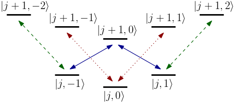
\lambda_{k}^{j}:=|E_{k+1}^{j+1}-E_{k}^{j}|=\Big|\frac{j+1}{I_{2}}+\Big(\frac{1}{2I_{3}}-\frac{1}{2I_{2}}\Big)(2k+1)\Big|,\quad k=-j,\dots,j,

(20)

corresponding to pairings for which both $j$ and $k$ move (see Figure 1),

\eta_{k}:=|E_{k+1}^{j}-E_{k}^{j}|=\Big|\Big(\dfrac{1}{2I_{3}}-\dfrac{1}{2I_{2}}\Big)(2k+1)\Big|,\quad k=-j,\dots,j,

(21)

and

\sigma^{j}:=|E_{k}^{j+1}-E_{k}^{j}|=\dfrac{j+1}{I_{2}},\quad k=-j,\dots,j,

(22)

for which, respectively, only $k$ or $j$ moves (see, Figures 2 2 and 2 2).

Refer to caption — Figure 1: Graph of the transitions associated with the frequency $\lambda_{k}^{j}$ between eigenstates $|j,k\rangle=|j,k,m\rangle:=D_{k,m}^{j}$ ( $m$ fixed). Same-shaped arrows correspond to equal spectral gaps.

We now classify the spectral gaps in terms of the sets $\Xi_{j}^{0}$ and $\Xi_{j}^{1}$ introduced in Section 3.1.

Lemma 14.

Let $I_{2}/I_{3}\notin\mathbb{Q}$ . Then $(\lambda_{k}^{j},l),(\sigma^{j},l)\in\Xi_{j}^{0}$ , and $(\eta_{k},l)\in\Xi_{j}^{1}$ , for all $k=-j,\dots,j$ , $l=1,2,3$ .

Proof.

Because of the selection rules (19), we only need to check if there are common spectral gaps in the spaces $\mathcal{M}_{j}$ and $\mathcal{M}_{j^{\prime}}$ for $j^{\prime}\neq j$ .

We start by proving that $(\lambda_{k}^{j},l),(\sigma^{j},l)\in\Xi_{j}^{0}$ by showing that a spectral gap of the type $\lambda_{k}^{j}$ (respectively, $\sigma^{j}$ ) is different from any spectral gap of the type $\lambda_{k^{\prime}}^{j^{\prime}}$ , $\sigma^{j^{\prime}}$ , or $\eta_{k^{\prime}}$ unless $\lambda_{k}^{j}=\lambda_{k^{\prime}}^{j^{\prime}}$ and $(k,j)=(k^{\prime},j^{\prime})$ (respectively, $\sigma^{j}=\sigma^{j^{\prime}}$ and $j=j^{\prime}$ ).

Using the explicit structure of the spectrum (16), any spectral gap of the type $\lambda_{k^{\prime}}^{j^{\prime}}$ , $\sigma^{j^{\prime}}$ , or $\eta_{k^{\prime}}$ can be written as

\Big|\frac{q_{1}}{I_{2}}+q_{2}\Big(\dfrac{1}{I_{3}}-\dfrac{1}{I_{2}}\Big)\Big|,\qquad q_{1},q_{2}\in\mathbb{Q}.

Since, moreover, $\frac{1}{I_{2}}$ and $\left(\frac{1}{I_{3}}-\frac{1}{I_{2}}\right)$ are $\mathbb{Q}$ -linearly independent, one easily deduces that, indeed, $(\lambda_{k}^{j},l),(\sigma^{j},l)\in\Xi_{j}^{0}$ .

Notice that the gaps of the type $\eta_{k}$ correspond to internal pairings in the spaces ${\cal H}_{j}$ . Henceforth, in order to prove that $(\eta_{k},l)\in\Xi_{j}^{1}$ it is enough to check that $\eta_{k}$ is different from any gap of the type $\lambda_{k^{\prime}}^{j},\sigma^{j}$ . This fact has already been noticed in the proof of the first part of the statement. The proof of the lemma is then concluded. ∎

Next, we introduce the family of excited modes associated with the spectral gap $\lambda_{k}^{j}$ , that is,

\mathcal{F}_{j}:=\{\mathcal{E}_{\lambda_{k}^{j}}(\mathrm{i}B_{l}),W_{\mathrm{i}}(\mathcal{E}_{\lambda_{k}^{j}}(\mathrm{i}B_{l}))\mid l=1,2,3,\;k=-j,\dots,j\},

where the operators $\mathcal{E}_{\mu}$ and $W_{\xi}$ are defined in Section 3.1, and where, with a slight abuse of notation, we write $B_{l}$ instead of $\Pi_{\mathcal{M}_{j}}B_{l}\Pi_{\mathcal{M}_{j}}$ . Notice that $\mathcal{F}_{j}\subset\nu_{j}^{0}$ as it follows from Lemma 14, where $\nu_{j}^{0}$ is defined as in (9).

In order to write down the matrices in $\mathcal{F}_{j}$ , we need to study the resonances between the spectral gaps inside $\mathcal{M}_{j}$ . We claim that there are no internal resonances except those due to the degeneracy $E_{k}^{j}=E_{-k}^{j}$ . Indeed, we already noticed in Lemma 14 that a spectral gap of the type $\lambda_{k}^{j}$ is different from any spectral gap of the type $\lambda_{k^{\prime}}^{j^{\prime}}$ , $\sigma^{j^{\prime}}$ , or $\eta_{k^{\prime}}$ unless $\lambda_{k}^{j}=\lambda_{k^{\prime}}^{j^{\prime}}$ and $(k,j)=(k^{\prime},j^{\prime})$ . We collect in the lemma below also the similar observations that $\sigma^{j}$ is different from any spectral gap of the type $\lambda_{k^{\prime}}^{j^{\prime}}$ , $\sigma^{j^{\prime}}$ , or $\eta_{k^{\prime}}$ unless $\sigma^{j}=\sigma^{j^{\prime}}$ and $j=j^{\prime}$ , and that $\eta_{k}\neq\eta_{k^{\prime}}$ if $k\neq k^{\prime}$ .

Lemma 15.

Let $I_{2}/I_{3}\notin\mathbb{Q}$ . Then

$\lambda_{k}^{j}$ -resonances: the equation

|E_{k+1}^{j+1}-E_{k}^{j}|=|E_{s+h}^{j^{\prime\prime}}-E_{s}^{j^{\prime}}|,\ j\leq j^{\prime}\leq j^{\prime\prime}\leq j+1,\ -j^{\prime}\leq s\leq j^{\prime},\ h\in\{-1,0,1\},

implies that $j^{\prime}=j$ , $j^{\prime\prime}=j+1$ , $s=\pm k$ , $s+h=\pm(k+1)$ ;

$\eta_{k}$ -resonances: the equation

|E_{k+1}^{j}-E_{k}^{j}|=|E_{s+h}^{j^{\prime\prime}}-E_{s}^{j^{\prime}}|,\ j\leq j^{\prime}\leq j^{\prime\prime}\leq j+1,\ -j^{\prime}\leq s\leq j^{\prime},\ h\in\{-1,0,1\},

implies that $j^{\prime}=j^{\prime\prime}=j$ or $j^{\prime}=j^{\prime\prime}=j+1$ and $s=\pm k$ , $s+h=\pm(k+1)$ ;

$\sigma^{j}$ -resonances: the equation

|E_{k}^{j+1}-E_{k}^{j}|=|E_{s+h}^{j^{\prime\prime}}-E_{s}^{j^{\prime}}|,\ j\leq j^{\prime}\leq j^{\prime\prime}\leq j+1,\ -j^{\prime}\leq s\leq j^{\prime},\ h\in\{-1,0,1\},

implies that $j^{\prime}=j$ , $j^{\prime\prime}=j+1$ , $h=0$ , $s=\pm k$ .

Denote by $\mathrm{L}_{j}:=\mathrm{Lie}(\mathcal{F}_{j})$ the Lie algebra generated by the matrices in $\mathcal{F}_{j}$ . Let us introduce the generalized Pauli matrices

G_{j,k}=e_{j,k}-e_{k,j},\quad F_{j,k}=\mathrm{i}e_{j,k}+\mathrm{i}e_{k,j},\quad D_{j,k}=\mathrm{i}e_{j,j}-\mathrm{i}e_{k,k},

where $e_{j,k}$ denotes the $(2j+1)^{2}+(2(j+1)+1)^{2}$ -square matrix whose entries are all zero, except the one at row $j$ and column $k$ , which is equal to $1$ . Consider again the lexicographic ordering $\rho:\{(l,k,m)\mid l=j,j+1,\;k,m=-l,\dots,l\}\rightarrow\mathbb{N}$ . By a slight abuse of notation, also set $e_{(l,k,m),(l^{\prime},k^{\prime},m^{\prime})}=e_{\rho(l,k,m),\rho(l^{\prime},k^{\prime},m^{\prime})}$ . The analogous identification can be used to define $G_{(l,k,m),(l^{\prime},k^{\prime},m^{\prime})},F_{(l,k,m),(l^{\prime},k^{\prime},m^{\prime})},D_{(l,k,m),(l^{\prime},k^{\prime},m^{\prime})}$ . The next proposition tells us how the elements in $\mathrm{L}_{j}$ look like. For a proof, see Appendix A.

Proposition 16.

Let $m=-j,\dots,j$ and $k=-j,\dots,j$ with $k\neq 0$ . Then the matrices $X_{(j,k,m),(j+1,k+1,m)}-X_{(j,-k,m),(j+1,-k-1,m)}$ and $X_{(j,k,m),(j+1,k+1,m\pm 1)}-X_{(j,-k,m),(j+1,-k-1,m\pm 1)}$ are in $\mathrm{L}_{j}$ , where $X\in\{G,F\}$ .

To break the degeneracy between $k$ and $-k$ which appears in the matrices that we found in Proposition 16, and obtain all the elementary matrices that one needs to generate $\mathfrak{su}(\mathcal{M}_{j})$ , we need to exploit the other two types of spectral gaps that we have introduced in (21) and (22) (see Figure 2).

Let us introduce the family of excited modes at the frequencies $\sigma^{j}$ and $\eta_{k}$ ,

\displaystyle\mathcal{P}_{j}:=\{\mathcal{E}_{\sigma^{j}}(\mathrm{i}B_{l}),W_{\mathrm{i}}(\mathcal{E}_{\sigma^{j}}(\mathrm{i}B_{l})),\mathcal{E}_{\eta_{k}}(\mathrm{i}B_{l}),W_{\mathrm{i}}(\mathcal{E}_{\eta_{k}}(\mathrm{i}B_{l}))\mid l=1,2,3,\;k=-j,\dots,j\},

and notice that, by Lemma 14, $\mathcal{P}_{j}\subset\nu_{j}^{1}$ (cf. (9)). Therefore,

\widetilde{\mathcal{P}}_{j}:=\{A,[B,C]\mid A,B\in\mathrm{L}_{j},C\in\mathcal{P}_{j}\}\subset\mathcal{T}_{j},

where we recall that $\mathcal{T}_{j}$ is the minimal ideal of $\mathrm{Lie}(\nu_{j}^{1})$ containing $\nu_{j}^{0}$ .

The following proposition, whose proof is given in Appendix B, concludes the proof of Theorem 13.

Proposition 17.

$\mathrm{Lie}(\widetilde{\mathcal{P}}_{j})=\mathfrak{su}(\mathcal{M}_{j})$ .

∎

Remark 18.

The assumption $I_{2}/I_{3}\notin\mathbb{Q}$ on the moments of inertia appearing in Theorem 13 is technical, and prevents the system from having both external resonances (as we saw in Lemma 14) and internal ones ( Lemma 15). Anyway, we have not proven that controllability fails if the ratio $I_{2}/I_{3}$ is rational.

3.5 Reachable sets of the quantum genuine symmetric-top

In (18) we see that, when $\delta=(0,0,\delta_{3})^{T}$ , transitions $k\rightarrow k^{\prime}$ are forbidden if $k\neq k^{\prime}$ . Thus, if the quantum system is prepared in the initial state $\psi(0)$ with $P_{3}\psi(0)=k\psi(0)$ , the wave function $\psi$ evolves in the subspaces $S_{k}=\overline{\mathrm{span}}\{D_{k,m}^{j}\mid j\in\mathbb{N},m=-j,\dots,j\}$ . The next theorem tells us that the restriction of (17) to this subspace is approximately controllable.

Theorem 19.

Let $I_{1}=I_{2}$ and fix $k\in\mathbb{Z}$ . If $\delta=(0,0,\delta_{3})^{T}$ , $\delta_{3}\neq 0$ , then the Schrödinger equation (17) is an m-tracker in the Hilbert space $S_{k}$ . In particular, $\mathrm{Reach}(\psi)$ is dense in $S_{k}\cap\mathcal{S}$ for all $\psi\in S_{k}\cap\mathcal{S}$ .

Proof.

For every integer $j\geq|k|$ , let $I_{j,k}:=\{\rho(l,m)\mid l=j,j+1,\;m=-l,\dots,l\}$ , where $\rho:\{(l,m)\mid l\geq|k|,\;m=-l,\dots,l\}\rightarrow\mathbb{N}$ is the lexicographic ordering. Then the graph $\mathcal{G}_{k}$ with vertices $\{I_{j,k}\}_{j=|k|}^{\infty}$ and edges $\{(I_{j,k},I_{j^{\prime},k})\mid I_{j,k}\cap I_{j^{\prime},k}\neq\emptyset\}$ is linear.

In order to apply Theorem 10 to the restriction of (17) to $S_{k}$ , we should consider the projected dynamics onto $\mathcal{N}_{j,k}:=\mathcal{L}_{j,k}\oplus\mathcal{L}_{j+1,k}$ , where $\mathcal{L}_{l,k}:=\mathrm{span}\{D_{k,m}^{l}\mid m=-l,\dots,l\}$ . The only spectral gaps in $S_{k}$ are $\sigma^{j}=|E_{k}^{j+1}-E_{k}^{j}|=\frac{j+1}{I_{2}}$ , $j\geq|k|$ . Notice that $(\sigma^{j},l)\in\Xi_{j}^{0}$ .

We write the electric potentials projected onto $\mathcal{N}_{j,k}$ :

		$\displaystyle\mathcal{E}_{\sigma^{j}}(\mathrm{i}B_{1})=\sum_{m=-j,\dots,j}a_{j,k,m}\delta_{3}G_{(j,k,m),(j+1,k,m+1)}+a_{j,k,-m}\delta_{3}G_{(j,k,m),(j+1,k,m-1)},$
		$\displaystyle\mathcal{E}_{\sigma^{j}}(\mathrm{i}B_{2})=\sum_{m=-j,\dots,j}a_{j,k,m}\delta_{3}F_{(j,k,m),(j+1,k,m+1)}-a_{j,k,-m}\delta_{3}F_{(j,k,m),(j+1,k,m-1)},$
		$\displaystyle\mathcal{E}_{\sigma^{j}}(\mathrm{i}B_{3})=\sum_{m=-j,\dots,j}-b_{j,k,m}\delta_{3}F_{(j,k,m),(j+1,k,m)},$

having used the explicit pairings (35), which can be found in Appendix B, and which describe the transitions excited by the frequency $\sigma^{j}$ . Note that here the sum does not run over $k$ since we are considering the dynamics restricted to $S_{k}$ . We consider the family of excited modes

\mathcal{F}_{j,k}=\{\mathcal{E}_{\sigma^{j}}(\mathrm{i}B_{l}),W_{\mathrm{i}}(\mathcal{E}_{\sigma^{j}}(\mathrm{i}B_{l}))\mid l=1,2,3\}\subset\nu_{j}^{0}.

We claim that the Lie algebra generated by $\mathcal{F}_{j,k}$ , seen as a subset of $\mathfrak{su}((2j+1)^{2}+(2(j+1)+1)^{2})$ , is equal to $\mathfrak{su}((2j+1)^{2}+(2(j+1)+1)^{2})$ . Such an identity has been proved in [8, Section 3.3], since the projection to $\mathcal{N}_{j,k}$ is isomorphic to an analogous projection for the linear molecule. Hence, we conclude that system (17) is an m-tracker in $S_{k}$ . ∎

3.6 Non-controllability of the quantum orthogonal accidentally symmetric-top

Let us consider separately the case where $\delta=(\delta_{1},\delta_{2},0)^{T}$ , left out by Theorem 13. The situation in which the dipole lies in the plane orthogonal to the symmetry axis of the molecule (that is, the orthogonal accidentally symmetric-top) is interesting from the point of view of chemistry, since the accidentally symmetric-top molecules present in nature are usually of that kind (see Figure 3).

In order to study this problem, let us introduce the Wang functions [19, Section 7.2]

S_{0,m,0}^{j}:=D_{0,m}^{j},,\qquad S_{k,m,\gamma}^{j}:=\dfrac{1}{\sqrt{2}}(D_{k,m}^{j}+(-1)^{\gamma}D_{-k,m}^{j}),\quad k=1,\dots,j,

for $j\in\mathbb{N}$ , $m=-j,\dots,j$ , and $\gamma=0,1$ . Due to the $k$ -degeneracy $E_{k}^{j}=E_{-k}^{j}$ in the spectrum of the rotational Hamiltonian $H$ , the functions $S_{k,m,\gamma}^{j}$ still form an orthogonal basis of eigenfunctions of $H$ . Then we consider the change of basis $D_{k,m}^{j}\rightarrow e^{-\mathrm{i}k\theta}D_{k,m}^{j}$ , and we choose $\theta\in[0,2\pi)$ such that

\begin{cases}e^{-\mathrm{i}\theta}(\delta_{2}+\mathrm{i}\delta_{1})=\mathrm{i}\sqrt{\delta_{1}^{2}+\delta_{2}^{2}},&\\ e^{\mathrm{i}\theta}(\delta_{2}-\mathrm{i}\delta_{1})=-\mathrm{i}\sqrt{\delta_{1}^{2}+\delta_{2}^{2}}.&\end{cases}

(23)

System (23) describes the rotation of angle $\mp\theta$ in the complex plane of the vector $\delta_{2}\pm\mathrm{i}\delta_{1}$ . The composition of these two changes of basis gives us the rotated Wang states $S_{k,m,\gamma}^{j}(\theta):=\frac{1}{\sqrt{2}}(e^{-\mathrm{i}k\theta}D_{k,m}^{j}+(-1)^{\gamma}e^{\mathrm{i}k\theta}D_{-k,m}^{j})$ , for $k\neq 0$ , and $S_{0,m,0}^{j}=D_{0,m}^{j}$ .

In the next theorem we express in this new basis a symmetry which prevents the system from being approximately controllable.

Theorem 20.

Let $I_{1}=I_{2}$ and $\delta=(\delta_{1},\delta_{2},0)^{T}$ . Then the parity of $j+\gamma+k$ is conserved, that is, the spaces $\overline{\mathrm{span}}\{S_{k,m,\gamma}^{j}\mid j+\gamma+k\mbox{ is odd}\}$ and $\overline{\mathrm{span}}\{S_{k,m,\gamma}^{j}\mid j+\gamma+k\mbox{ is even}\}$ are invariant for the propagators of (17).

Proof.

We need to prove that the pairings allowed by the controlled vector fields $B_{1},B_{2}$ and $B_{3}$ conserve the parity of $j+\gamma+k$ . To do so, let us compute

$\displaystyle\langle S_{k,m,\gamma}^{j}(\theta),\mathrm{i}B_{1}S_{k+1,m+1,\gamma}^{j+1}(\theta)\rangle$	$\displaystyle=-c_{j,k,m}e^{-\mathrm{i}\theta}(\delta_{2}+\mathrm{i}\delta_{1})+c_{j,k,m}e^{\mathrm{i}\theta}(\delta_{2}-\mathrm{i}\delta_{1})$
	$\displaystyle=-2\mathrm{i}c_{j,k,m}\sqrt{\delta_{1}^{2}+\delta_{2}^{2}},$	(24)
$\displaystyle\langle S_{k,m,\gamma}^{j}(\theta),\mathrm{i}B_{1}S_{k+1,m+1,\gamma^{\prime}}^{j+1}(\theta)\rangle$	$\displaystyle=-c_{j,k,m}e^{-\mathrm{i}\theta}(\delta_{2}+\mathrm{i}\delta_{1})-c_{j,k,m}e^{\mathrm{i}\theta}(\delta_{2}-\mathrm{i}\delta_{1})$
	$\displaystyle=0,\qquad\gamma\neq\gamma^{\prime},$

having used the expression of the Wang functions as linear combinations of Wigner functions, the explicit pairings (27) which can be found in Appendix A, and the choice of $\theta$ made in (23). Then we also have

\begin{cases}\langle S_{k,m,\gamma}^{j}(\theta),\mathrm{i}B_{1}S_{k+1,m+1,\gamma}^{j}(\theta)\rangle=0,&\\ \langle S_{k,m,\gamma}^{j}(\theta),\mathrm{i}B_{1}S_{k+1,m+1,\gamma^{\prime}}^{j}(\theta)\rangle=-2\mathrm{i}h_{j,k,m}\sqrt{\delta_{1}^{2}+\delta_{2}^{2}},\quad\gamma\neq\gamma^{\prime},&\end{cases}

(25)

having used this time the pairings (34), which can be found in Appendix B. From (24) and (25) we can see that the allowed transitions only depend on the parity of $j+\gamma$ and $k$ ; indeed, we have either transitions between states of the form

\begin{cases}j+\gamma&\text{even}\\ k&\text{even}\\ \end{cases}\longleftrightarrow\begin{cases}j^{\prime}+\gamma^{\prime}&\text{odd}\\ k^{\prime}&\text{odd},\end{cases}

or transitions between states of the form

\begin{cases}j+\gamma&\text{even}\\ k&\text{odd}\\ \end{cases}\longleftrightarrow\begin{cases}j^{\prime}+\gamma^{\prime}&\text{odd}\\ k^{\prime}&\text{even}.\end{cases}

The same happens if we replace $m+1$ with $m-1$ and $k+1$ with $k-1$ in (24) and (25). Because of the selection rules (19), these are the only transitions allowed by the field $B_{1}$ . One can easily check, in the same way, that every transition induced by $B_{2},B_{3}$ also conserves the parity of $j+\gamma+k$ . ∎

Appendix A Proof of Proposition 16

As a consequence of Lemma 15, part 1, if $I_{2}/I_{3}\notin\mathbb{Q}$ , the only transitions driven by the fields $\mathrm{i}B_{l}$ , $l=1,2,3$ , excited at frequency $\lambda_{k}^{j}$ , are the ones corresponding to the following matrix elements (written in the basis of $\mathcal{M}_{j}$ given by the Wigner functions) and can be computed using, e.g., [19, Table 2.1]:

\begin{cases}\langle D_{k,m}^{j},\mathrm{i}B_{1}D_{k+1,m\pm 1}^{j+1}\rangle=-c_{j,k,\pm m}(\delta_{2}+\mathrm{i}\delta_{1}),&\\ \langle D_{k,m}^{j},\mathrm{i}B_{1}D_{k-1,m\pm 1}^{j+1}\rangle=c_{j,-k,\pm m}(\delta_{2}-\mathrm{i}\delta_{1}),&\\ \langle D_{k,m}^{j},\mathrm{i}B_{2}D_{k+1,m\pm 1}^{j+1}\rangle=\mp\mathrm{i}c_{j,k,\pm m}(\delta_{2}+\mathrm{i}\delta_{1}),&\\ \langle D_{k,m}^{j},\mathrm{i}B_{2}D_{k-1,m\pm 1}^{j+1}\rangle=\pm\mathrm{i}c_{j,-k,\pm m}(\delta_{2}-\mathrm{i}\delta_{1}),&\\ \langle D_{k,m}^{j},\mathrm{i}B_{3}D_{k\pm 1,m}^{j+1}\rangle=\pm\mathrm{i}d_{j,\pm k,m}(\delta_{2}\pm\mathrm{i}\delta_{1}),&\end{cases}

(26)

where

c_{j,k,m}:=\dfrac{[(j+k+1)(j+k+2)]^{1/2}[(j+m+1)(j+m+2)]^{1/2}}{4(j+1)[(2j+1)(2j+3)]^{1/2}},

and

d_{j,k,m}:=\dfrac{[(j+k+1)(j+k+2)]^{1/2}[(j+1)^{2}-m^{2}]^{1/2}}{2(j+1)[(2j+1)(2j+3)]^{1/2}}.

Now, using a symmetry argument, we explain how to get rid of one electric dipole component between $\delta_{1}$ and $\delta_{2}$ .

By the very definition of the Euler angles, one has that the rotation of angle $\theta$ around the symmetry axis $a_{3}$ is given by $\gamma\mapsto\gamma+\theta.$ This rotation acts on the Wigner functions in the following way

D_{k,m}^{j}(\alpha,\beta,\gamma)\mapsto D_{k,m}^{j}(\alpha,\beta,\gamma+\theta)=e^{\mathrm{i}k\theta}D_{k,m}^{j}(\alpha,\beta,\gamma)=:D_{k,m}^{j}(\theta)(\alpha,\beta,\gamma),

having used the explicit expression of the symmetric states (15). Note that these rotated Wigner functions form again an orthogonal basis for $L^{2}({\rm SO}(3))$ of eigenfunctions of the rotational Hamiltonian $H$ , so we can also analyze the controllability problem in this new basis. In this new basis the matrix elements (corresponding to the frequency $\lambda_{k}^{j}$ ) of the controlled fields are

\begin{cases}\langle D_{k,m}^{j}(\theta),\mathrm{i}B_{1}D_{k+1,m+1}^{j+1}(\theta)\rangle&=-c_{j,k,m}e^{-\mathrm{i}\theta}(\delta_{2}+\mathrm{i}\delta_{1}),\\ \langle D_{k,m}^{j}(\theta),\mathrm{i}B_{1}D_{k-1,m+1}^{j+1}(\theta)\rangle&=c_{j,-k,m}e^{\mathrm{i}\theta}(\delta_{2}-\mathrm{i}\delta_{1}),\end{cases}

(27)

and the same happens for all the other transitions described in (26). So, the effect of this change of basis is that we are actually rotating the first two components of the dipole moment, by the angle $\theta$ . We can now choose $\theta\in[0,2\pi)$ such that

e^{-\mathrm{i}\theta}(\delta_{2}+\mathrm{i}\delta_{1})=\sqrt{\delta_{1}^{2}+\delta_{2}^{2}}=e^{\mathrm{i}\theta}(\delta_{2}-\mathrm{i}\delta_{1}).

In other words, thanks to this change of basis, we can assume without loss of generality that $\delta_{1}=0$ , since we can rotate the vector $\delta_{2}\pm\mathrm{i}\delta_{1}$ and get rid of its imaginary part (note that in (23) and in the proof of Theorem 20 we are rotating the vector $\delta_{2}\pm\mathrm{i}\delta_{1}$ in the other sense, i.e., to get rid of its real part). This will simplify the expression of the controlled fields. Note that

		$\displaystyle W_{\mathrm{i}}(G_{(j,k,m),(j+1,k+1,n)})=-F_{(j,k,m),(j+1,k+1,n)},$
		$\displaystyle W_{\mathrm{i}}(F_{(j,k,m),(j+1,k+1,n)})=G_{(j,k,m),(j+1,k+1,n)}.$

From the identity $[e_{j,k},e_{n,m}]=\delta_{kn}e_{j,m}-\delta_{jm}e_{n,k}$ we get the bracket relations

[G_{j,k},G_{k,n}]=G_{j,n},\quad[F_{j,k},F_{k,n}]=-G_{j,n},\quad[G_{j,k},F_{k,n}]=F_{j,n},

[G_{j,k},F_{j,k}]=2D_{j,k},\quad[F_{j,k},D_{j,k}]=2G_{j,k}.

Moreover, two operators coupling no common states commute, that is,

[Y_{j,k},Z_{j^{\prime},k^{\prime}}]=0\qquad\text{ if }\{j,k\}\cap\{j^{\prime},k^{\prime}\}=\emptyset,

with $Y,Z\in\{G,F,D\}$ .

Finally, we can conveniently represent the matrices corresponding to the controlled vector field (projected onto $\mathcal{M}_{j}$ ) in the rotated basis found with the symmetry argument. So, for each $k=-j,\dots,j$ , because of Lemma 15, part 1, and (26), we have

	$\displaystyle\mathcal{E}_{\lambda_{k}^{j}}(\mathrm{i}B_{1})=$	$\displaystyle\sum_{m=-j,\dots,j}-c_{j,k,m}\delta_{2}G_{(j,k,m),(j+1,k+1,m+1)}-c_{j,k,-m}\delta_{2}G_{(j,k,m),(j+1,k+1,m-1)}$
		$\displaystyle+c_{j,k,m}\delta_{2}G_{(j,-k,m),(j+1,-k-1,m+1)}+c_{j,k,-m}\delta_{2}G_{(j,-k,m),(j+1,-k-1,m-1)},$		(28)

	$\displaystyle\mathcal{E}_{\lambda_{k}^{j}}(\mathrm{i}B_{2})=$	$\displaystyle\sum_{m=-j,\dots,j}-c_{j,k,m}\delta_{2}F_{(j,k,m),(j+1,k+1,m+1)}+c_{j,k,-m}\delta_{2}F_{(j,k,m),(j+1,k+1,m-1)}$
		$\displaystyle+c_{j,k,m}\delta_{2}F_{(j,-k,m),(j+1,-k-1,m+1)}-c_{j,k,-m}\delta_{2}F_{(j,-k,m),(j+1,-k-1,m-1)},$		(29)

\displaystyle\mathcal{E}_{\lambda_{k}^{j}}(\mathrm{i}B_{3})

\displaystyle=\sum_{m=-j,\dots,j}d_{j,k,m}\delta_{2}F_{(j,k,m),(j+1,k+1,m)}-d_{j,k,m}\delta_{2}F_{(j,-k,m),(j+1,-k-1,m)},

(30)

where, with a slight abuse of notation, we write $B_{l}$ instead of $\Pi_{\mathcal{M}_{j}}B_{l}\Pi_{\mathcal{M}_{j}}$ .

Now we show how the sum over $m$ in (28), (29) and (30) can be decomposed, in order to obtain that the matrices $X_{(j,k,m),(j+1,k+1,m\pm 1)}+X_{(j,-k,m),(j+1,-k-1,m\pm 1)}$ and $X_{(j,k,m),(j+1,k+1,m)}-X_{(j,-k,m),(j+1,-k-1,m)}$ are in $\mathrm{L}_{j}$ , for any $m,k=-j,\dots,j$ , where $X\in\{G,F\}$ . Let us first fix $k\neq 0$ and consider

	$\displaystyle W_{\mathrm{i}}(\mathcal{E}_{\lambda_{k}^{j}}$	$\displaystyle(\mathrm{i}B_{3}))$
		$\displaystyle=\sum_{m=-j,\dots,j}d_{j,k,m}\delta_{2}G_{(j,k,m),(j+1,k+1,m)}-d_{j,k,m}\delta_{2}G_{(j,-k,m),(j+1,-k-1,m)},$

and the brackets

	$\displaystyle\mathrm{ad}_{\mathcal{E}_{\lambda_{k}^{j}}(\mathrm{i}B_{3})}^{2s}(W_{\mathrm{i}}(\mathcal{E}_{\lambda_{k}^{j}}(\mathrm{i}B_{3})))=$	$\displaystyle\sum_{m=-j,\dots,j}(-1)^{s}2^{2s}d_{j,k,m}^{2s+1}\delta_{2}^{2s+1}G_{(j,k,m),(j+1,k+1,m)}$
		$\displaystyle+(-1)^{s}2^{2s}(-d_{j,k,m})^{2s+1}\delta_{2}^{2s+1}G_{(j,-k,m),(j+1,-k-1,m)},$

for $s\in\mathbb{N}$ , where $\mathrm{ad}_{A}(B)=[A,B]$ and $\mathrm{ad}_{A}^{n+1}(B)=[A,\mathrm{ad}_{A}^{n}(B)]$ . Since $d_{j,k,m}=d_{j,k,-m}$ , the invertibility of the Vandermonde matrix gives that

		$\displaystyle G_{(j,k,m),(j+1,k+1,m)}+G_{(j,k,-m),(j+1,k+1,-m)}$
	$\displaystyle-$	$\displaystyle G_{(j,-k,m),(j+1,-k-1,m)}-G_{(j,-k,-m),(j+1,-k-1,-m)}\in\mathrm{L}_{j},$		(31)

for $m=0,\dots,j$ . In particular, $G_{(j,k,0),(j+1,k+1,0)}-G_{(j,-k,0),(j+1,-k-1,0)}$ is in $\mathrm{L}_{j}$ . Hence,

		$\displaystyle\Big[\Big[\dfrac{\mathcal{E}_{\lambda_{k}}(\mathrm{i}B_{1})-W_{\mathrm{i}}(\mathcal{E}_{\lambda_{k}}(\mathrm{i}B_{2}))}{2},G_{(j,k,0),(j+1,k+1,0)}-G_{(j,-k,0),(j+1,-k-1,0)}\Big],$		(32)
		$\displaystyle G_{(j,k,0),(j+1,k+1,0)}-G_{(j,-k,0),(j+1,-k-1,0)}\Big]=c_{j,k,0}\delta_{2}G_{(j,k,0),(j+1,k+1,-1)}$
		$\displaystyle+c_{j,k,-1}\delta_{2}G_{(j,k,1),(j+1,k+1,0)}-c_{j,k,0}\delta_{2}G_{(j,-k,0),(j+1,-k-1,-1)}$
		$\displaystyle-c_{j,k,-1}\delta_{2}G_{(j,-k,1),(j+1,-k-1,0)}$

is also in $\mathrm{L}_{j}$ . Define

	$\displaystyle Q_{0}=$	$\displaystyle c_{j,k,0}\delta_{2}G_{(j,k,0),(j+1,k+1,-1)}+c_{j,k,-1}\delta_{2}G_{(j,k,1),(j+1,k+1,0)}$
		$\displaystyle-c_{j,k,0}\delta_{2}G_{(j,-k,0),(j+1,-k-1,-1)}-c_{j,k,-1}\delta_{2}G_{(j,-k,1),(j+1,-k-1,0)},$
	$\displaystyle Q_{m}=$	$\displaystyle c_{j,k,-m}\delta_{2}G_{(j,k,-m),(j+1,k+1,-m-1)}+c_{j,k,-m-1}\delta_{2}G_{(j,k,m+1),(j+1,k+1,m)}$
		$\displaystyle-c_{j,k,-m}\delta_{2}G_{(j,-k,-m),(j+1,-k-1,-m-1)}-c_{j,k,-m-1}\delta_{2}G_{(j,-k,m+1),(j+1,-k-1,m)},$

if $0<m<j$ , and

Q_{j}=c_{j,k,-j}\delta_{2}G_{(j,k,-j),(j+1,k+1,-j-1)}-c_{j,k,-j}\delta_{2}G_{(j,-k,-j),(j+1,-k-1,-j-1)}.

We have

		$\displaystyle\Big[\Big[\sum_{m=s,\dots,j}Q_{m},G_{(j,k,s),(j+1,k+1,s)}+G_{(j,k,-s),(j+1,k+1,-s)}-G_{(j,-k,s),(j+1,-k-1,s)}$
		$\displaystyle-G_{(j,-k,-s),(j+1,-k-1,-s)}\Big],G_{(j,k,s),(j+1,k+1,s)}+G_{(j,k,-s),(j+1,k+1,-s)}$
		$\displaystyle-G_{(j,-k,s),(j+1,-k-1,s)}-G_{(j,-k,-s),(j+1,-k-1,-s)}\Big]=Q_{s},$

for $s=1,\dots,j$ . By iteration on $s$ and because of (31), it follows that $Q_{s}\in\mathrm{L}_{j}$ for every $s=0,\dots,j$ . Now, since

\dfrac{Q_{j}}{c_{j,k,-j}\delta_{2}}=G_{(j,k,-j),(j+1,k+1,-j-1)}-G_{(j,-k,-j),(j+1,-k-1,-j-1)}\in\mathrm{L}_{j},

then

		$\displaystyle\mathrm{ad}_{G_{(j,k,-j),(j+1,k+1,-j-1)}-G_{(j,-k,-j),(j+1,-k-1,-j-1)}}^{2}(G_{(j,k,j),(j+1,k+1,j)}$
		$\displaystyle+G_{(j,k,-j),(j+1,k+1,-j)}-G_{(j,-k,j),(j+1,-k-1,j)}-G_{(j,-k,-j),(j+1,-k-1,-j)})$
		$\displaystyle=G_{(j,k,-j),(j+1,k+1,-j)}-G_{(j,-k,-j),(j+1,-k-1,-j)}\in\mathrm{L}_{j},$

which, in turns, implies that

		$\displaystyle\mathrm{ad}_{G_{(j,k,-j),(j+1,k+1,-j)}-G_{(j,-k,-j),(j+1,-k-1,-j)}}^{2}(Q_{j-1})$
		$\displaystyle=c_{j,k,-j+1}G_{(j,k,-j+1),(j+1,k+1,-j)}-c_{j,k,-j+1}G_{(j,-k,-j+1),(j+1,-k-1,-j)}\in\mathrm{L}_{j}.$

Iterating the argument,

G_{(j,k,m),(j+1,k+1,m)}-G_{(j,-k,m),(j+1,-k-1,m)}\in\mathrm{L}_{j},\quad m=-j,\dots,j

(33)

and $G_{(j,k,m),(j+1,k+1,m-1)}-G_{(j,-k,m),(j+1,-k-1,m-1)}$ are in $\mathrm{L}_{j}$ for $m=-j,\dots,j$ .

By the same argument as above, with $\frac{\mathcal{E}_{\lambda_{k}^{j}}(\mathrm{i}B_{1})-W_{\mathrm{i}}(\mathcal{E}_{\lambda_{k}^{j}}(\mathrm{i}B_{2}))}{2}$ replaced by

	$\displaystyle\dfrac{\mathcal{E}_{\lambda_{k}^{j}}(\mathrm{i}B_{1})+W_{\mathrm{i}}(\mathcal{E}_{\lambda_{k}^{j}}(\mathrm{i}B_{2}))}{2}=$	$\displaystyle\sum_{m=-j,\dots,j}-c_{j,k,m}G_{(j,k,m),(j+1,k+1,m+1)}$
		$\displaystyle+c_{j,k,m}G_{(j,-k,m),(j+1,-k-1,m+1)}$

in (32) we also have that $G_{(j,k,m),(j+1,k+1,m+1)}-G_{(j,-k,m),(j+1,-k-1,m+1)}$ is in $\mathrm{L}_{j}$ for all $m=-j,\dots,j$ .

If we now replace $\frac{\mathcal{E}_{\lambda_{k}^{j}}(\mathrm{i}B_{1})-W_{\mathrm{i}}(\mathcal{E}_{\lambda_{k}^{j}}(\mathrm{i}B_{2}))}{2}$ with

	$\displaystyle\dfrac{\mathcal{E}_{\lambda_{k}^{j}}(\mathrm{i}B_{2})+W_{\mathrm{i}}(\mathcal{E}_{\lambda_{k}^{j}}(\mathrm{i}B_{1}))}{2}=$	$\displaystyle\sum_{m=-j,\dots,j}-c_{j,k,-m}F_{(j,k,m),(j+1,k+1,m-1)}$
		$\displaystyle+c_{j,k,-m}F_{(j,-k,m),(j+1,-k-1,m-1)}$

	$\displaystyle\dfrac{\mathcal{E}_{\lambda_{k}^{j}}(\mathrm{i}B_{2})-W_{\mathrm{i}}(\mathcal{E}_{\lambda_{k}^{j}}(\mathrm{i}B_{1}))}{2}=$	$\displaystyle\sum_{m=-j,\dots,j}-c_{j,k,m}F_{(j,k,m),(j+1,k+1,m+1)}$
		$\displaystyle+c_{j,k,m}F_{(j,-k,m),(j+1,-k-1,m+1)},$

the arguments above prove that both $F_{(j,k,m),(j+1,k+1,m)}-F_{(j,-k,m),(j+1,-k-1,m)}$ and $F_{(j,k,m),(j+1,k+1,m\pm 1)}-F_{(j,-k,m),(j+1,-k-1,m\pm 1)}$ are in $\mathrm{L}_{j}$ for all $m=-j,\dots,j$ .

Appendix B Proof of Proposition 17

Using again [19, Table 2.1] we write the pairings

\begin{cases}\langle D_{k,m}^{j},\mathrm{i}B_{1}D_{k+1,m\pm 1}^{j}\rangle=\mp h_{j,k,\pm m}(\delta_{2}+\mathrm{i}\delta_{1}),&\\ \langle D_{k,m}^{j},\mathrm{i}B_{1}D_{k-1,m\pm 1}^{j}\rangle=\mp h_{j,-k,\pm m}(\delta_{2}-\mathrm{i}\delta_{1}),&\\ \langle D_{k,m}^{j},\mathrm{i}B_{2}D_{k+1,m\pm 1}^{j}\rangle=-\mathrm{i}h_{j,k,\pm m}(\delta_{2}+\mathrm{i}\delta_{1}),&\\ \langle D_{k,m}^{j},\mathrm{i}B_{2}D_{k-1,m\pm 1}^{j}\rangle=-\mathrm{i}h_{j,-k,\pm m}(\delta_{2}-\mathrm{i}\delta_{1}),&\\ \langle D_{k,m}^{j},\mathrm{i}B_{3}D_{k\pm 1,m}^{j}\rangle=-\mathrm{i}q_{j,\pm k,m}(\delta_{2}\pm\mathrm{i}\delta_{1}),&\end{cases}

(34)

where

	$\displaystyle h_{j,k,m}$	$\displaystyle:=\dfrac{[j(j+1)-k(k+1)]^{1/2}[j(j+1)-m(m+1)]^{1/2}}{4j(j+1)},$
	$\displaystyle q_{j,k,m}$	$\displaystyle:=\dfrac{[j(j+1)-k(k+1)]^{1/2}m}{2j(j+1)}.$

Moreover,

\begin{cases}\langle D_{k,m}^{j},\mathrm{i}B_{1}D_{k,m\pm 1}^{j+1}\rangle=a_{j,k,\pm m}\delta_{3},&\\ \langle D_{k,m}^{j},\mathrm{i}B_{2}D_{k,m\pm 1}^{j+1}\rangle=\pm\mathrm{i}a_{j,k,\pm m}\delta_{3},&\\ \langle D_{k,m}^{j},\mathrm{i}B_{3}D_{k,m}^{j+1}\rangle=-\mathrm{i}b_{j,k,m}\delta_{3},&\end{cases}

(35)

where

	$\displaystyle a_{j,k,m}$	$\displaystyle:=\dfrac{[(j+1)^{2}-k^{2}]^{1/2}[(j+m+1)(j+m+2)]^{1/2}}{2(j+1)[(2j+1)(2j+3)]^{1/2}},$
	$\displaystyle b_{j,k,m}$	$\displaystyle:=\dfrac{[(j+1)^{2}-k^{2}]^{1/2}[(j+1)^{2}-m^{2}]^{1/2}}{(j+1)[(2j+1)(2j+3)]^{1/2}}.$

Note that the $k\rightarrow k$ transitions are driven by $\delta_{3}$ . Recall that, up to a rotation, we can assume that $\delta_{1}=0$ . Because of Lemma 15, parts 2 and 3, the expression of the controlled fields excited at the frequencies $\eta_{k}$ and $\sigma^{j}$ are

	$\displaystyle\mathcal{E}_{\eta_{k}}(\mathrm{i}B_{1})=$	$\displaystyle\sum_{\begin{subarray}{c}l=j,j+1,\\ m=-l,\dots,l-1\end{subarray}}-h_{l,k,m}\delta_{2}G_{(l,k,m),(l,k+1,m+1)}-h_{l,k,m}\delta_{2}G_{(l,-k,m),(l,-k-1,m+1)}$
		$\displaystyle\hskip-2.84526pt+\hskip-5.69054pt\sum_{\begin{subarray}{c}l=j,j+1,\\ m=-l+1,\dots,l\end{subarray}}h_{l,k,-m}\delta_{2}G_{(l,k,m),(l,k+1,m-1)}+h_{l,k,-m}\delta_{2}G_{(l,-k,m),(l,-k-1,m-1)},$		(36)

	$\displaystyle\mathcal{E}_{\eta_{k}}(\mathrm{i}B_{2})$	$\displaystyle=\sum_{\begin{subarray}{c}l=j,j+1,\\ m=-l,\dots,l-1\end{subarray}}-h_{l,k,m}\delta_{2}F_{(l,k,m),(l,k+1,m+1)}-h_{l,k,m}\delta_{2}F_{(l,-k,m),(l,-k-1,m+1)}$
		$\displaystyle+\hskip-2.84526pt\sum_{\begin{subarray}{c}l=j,j+1,\\ m=-l+1,\dots,l\end{subarray}}-h_{l,k,-m}\delta_{2}F_{(l,k,m),(l,k+1,m-1)}-h_{l,k,-m}\delta_{2}F_{(l,-k,m),(l,-k-1,m-1)},$		(37)

\mathcal{E}_{\eta_{k}}(\mathrm{i}B_{3})=\sum_{\begin{subarray}{c}l=j,j+1,\\ m=-l,\dots,l\end{subarray}}-q_{l,k,m}\delta_{2}F_{(l,k,m),(l,k+1,m)}-q_{l,k,m}\delta_{2}F_{(l,-k,m),(l,-k-1,m)},

(38)

and

		$\displaystyle\mathcal{E}_{\sigma^{j}}(\mathrm{i}B_{1})=\sum_{m,k=-j,\dots,j}a_{j,k,m}\delta_{3}G_{(j,k,m),(j+1,k,m+1)}+a_{j,k,-m}\delta_{3}G_{(j,k,m),(j+1,k,m-1)},$		(39)
		$\displaystyle\mathcal{E}_{\sigma^{j}}(\mathrm{i}B_{2})=\sum_{m,k=-j,\dots,j}a_{j,k,m}\delta_{3}F_{(j,k,m),(j+1,k,m+1)}-a_{j,k,-m}\delta_{3}F_{(j,k,m),(j+1,k,m-1)},$
		$\displaystyle\mathcal{E}_{\sigma^{j}}(\mathrm{i}B_{3})=\sum_{m,k=-j,\dots,j}-b_{j,k,m}\delta_{3}F_{(j,k,m),(j+1,k,m)}.$

Note that in $\mathcal{E}_{\eta_{k}}(-iB_{3})$ the term for $m=0$ vanishes, since $q_{j,k,0}=0$ for every $j,k$ .

To decouple all the $m$ -degeneracies in the excited modes, we just consider double brackets with the elementary matrices that we have obtained above. As an example, using (33) we can decouple the $m\rightarrow m$ transitions corresponding to the frequency $\sigma^{j}$ by considering

		$\displaystyle[[W_{\mathrm{i}}(\mathcal{E}_{\sigma^{j}}(\mathrm{i}B_{3})),G_{(j,k,m),(j+1,k+1,m)}-G_{(j,-k,m),(j+1,-k-1,m)}],$
		$\displaystyle G_{(j,k,m),(j+1,k+1,m)}-G_{(j,-k,m),(j+1,-k-1,m)}]$
		$\displaystyle=G_{(j,k,m),(j+1,k,m)}+G_{(j,-k,m),(j+1,-k,m)}\in\mathrm{Lie}(\widetilde{\mathcal{P}}_{j}).$

Considering every possible double brackets as above, we obtain, for $X\in\{G,F\}$ , that

X_{(j,k,m),(j+1,k,m)}+X_{(j,-k,m),(j+1,-k,m)}\in\mathrm{Lie}(\widetilde{\mathcal{P}}_{j}),\quad k\neq 0,

(40)

when we start from the matrices in (39), and that

X_{(l,k,m),(l,k+1,m)}+X_{(l,-k,m),(l,-k-1,m)},X_{(l,k,m),(l,k+1,m\pm 1)}+X_{(l,-k,m),(j,-k-1,m\pm 1)}

are in $\mathrm{Lie}(\widetilde{\mathcal{P}}_{j})$ , $l=j,j+1$ , $m,k\neq 0$ , when we start from the matrices in (36), (37), (38). Now we can also generate the missing $k=0$ elements of (33) by taking double brackets with $X_{(j+1,1,m),(j+1,2,m)}+X_{(j+1,-1,m),(j+1,-2,m)}\in\mathrm{Lie}(\widetilde{\mathcal{P}}_{j})$ . As an example, we have that

		$\displaystyle[[\mathcal{E}_{\lambda_{0}^{j}}(\mathrm{i}B_{3}),F_{(j+1,1,m),(j+1,2,m)}+F_{(j+1,-1,m),(j+1,-2,m)}],$
		$\displaystyle F_{(j+1,1,m),(j+1,2,m)}+F_{(j+1,-1,m),(j+1,-2,m)}]$
		$\displaystyle=F_{(j,0,m),(j+1,1,m)}-F_{(j,0,m),(j+1,-1,m)}\in\mathrm{Lie}(\widetilde{\mathcal{P}}_{j}).$

Moreover, also the $m=0$ elements in the transitions (38) are in $\mathrm{Lie}(\widetilde{\mathcal{P}}_{j})$ , as one can check by considering a bracket between two transitions obtained in (33) and (40). For example,

		$\displaystyle[G_{(j,k,0),(j+1,k+1,0)}-G_{(j,-k,0),(j+1,-k-1,0)},G_{(j+1,k+1,0),(j,k+1,0)}$
		$\displaystyle+G_{(j+1,-k-1,0),(j,-k-1,0)}]=G_{(j,k,0),(j,k+1,0)}-G_{(j,-k,0),(j,-k-1,0)}\in\mathrm{Lie}(\widetilde{\mathcal{P}}_{j}).$

Finally, we apply a three-wave mixing argument (Figure 4) in order to decouple the sum over $k$ and $-k$ in every elementary matrices: consider the bracket between the following elements in $\mathrm{Lie}(\widetilde{\mathcal{P}}_{j})$

		$\displaystyle[G_{(j,k+1,m),(j,k,m)}+G_{(j,-k-1,m),(j,-k,m)},G_{(j,k,m),(j+1,k,m)}+G_{(j,-k,m),(j+1,-k,m)}]$
		$\displaystyle=G_{(j,k+1,m),(j+1,k,m)}+G_{(j,-k-1,m),(j+1,-k,m)}\in\mathrm{Lie}(\widetilde{\mathcal{P}}_{j}),\quad k\neq 0,$

and notice that from (33) we already have that $G_{(j,k+1,m),(j+1,k,m)}-G_{(j,-k-1,m),(j+1,-k,m)}$ is in $\mathrm{Lie}(\widetilde{\mathcal{P}}_{j})$ , and hence $G_{(j,k+1,m),(j+1,k,m)}$ and $G_{(j,-k-1,m),(j+1,-k,m)}$ are in $\mathrm{Lie}(\widetilde{\mathcal{P}}_{j})$ . In this way we can break every $k$ -degeneracy, and finally obtain that $\mathrm{Lie}(\widetilde{\mathcal{P}}_{j})=\mathfrak{su}(\mathcal{M}_{j})$ , which concludes the proof.

References

[1] R. Abraham, J. E. Marsden, and T. Ratiu, Manifolds, tensor analysis, and applications, vol. 75 of Applied Mathematical Sciences, Springer-Verlag, New York, second ed., 1988.
[2] A. A. Agrachev and Y. L. Sachkov, Control theory from the geometric viewpoint, vol. 87 of Encyclopaedia of Mathematical Sciences, Springer-Verlag, Berlin, 2004. Control Theory and Optimization, II.
[3] C. Altafini and F. Ticozzi, Modeling and control of quantum systems: an introduction, IEEE Trans. Automat. Control, 57 (2012), pp. 1898–1917.
[4] I. Averbukh, E. Gershnabel, S. Goldl, and I. Tutunnikov, Selective orientation of chiral molecules by laser fields with twisted polarization, J. Phys. Chem. Lett., (2018), pp. 1105–1111.
[5] K. Beauchard and J.-M. Coron, Controllability of a quantum particle in a moving potential well, J. Funct. Anal., 232 (2006), pp. 328–389.
[6] A. M. Bloch, P. S. Krishnaprasad, J. E. Marsden, and G. Sánchez de Alvarez, Stabilization of rigid body dynamics by internal and external torques, Automatica J. IFAC, 28 (1992), pp. 745–756.
[7] U. Boscain, M. Caponigro, T. Chambrion, and M. Sigalotti, A weak spectral condition for the controllability of the bilinear Schrödinger equation with application to the control of a rotating planar molecule, Comm. Math. Phys., 311 (2012), pp. 423–455.
[8] U. Boscain, M. Caponigro, and M. Sigalotti, Multi-input Schrödinger equation: controllability, tracking, and application to the quantum angular momentum, J. Differential Equations, 256 (2014), pp. 3524–3551.
[9] U. Boscain, J.-P. Gauthier, F. Rossi, and M. Sigalotti, Approximate controllability, exact controllability, and conical eigenvalue intersections for quantum mechanical systems, Comm. Math. Phys., 333 (2015), pp. 1225–1239.
[10] U. Boscain, P. Mason, G. Panati, and M. Sigalotti, On the control of spin-boson systems, J. Math. Phys., 56 (2015), pp. 092101, 15.
[11] M. Caponigro and M. Sigalotti, Exact controllability in projections of the bilinear Schrödinger equation, SIAM J. Control Optim., 56 (2018), pp. 2901–2920.
[12] T. Chambrion, Periodic excitations of bilinear quantum systems, Automatica J. IFAC, 48 (2012), pp. 2040–2046.
[13] T. Chambrion, P. Mason, M. Sigalotti, and U. Boscain, Controllability of the discrete-spectrum Schrödinger equation driven by an external field, Ann. Inst. H. Poincaré Anal. Non Linéaire, 26 (2009), pp. 329–349.
[14] P. E. Crouch, Spacecraft attitude control and stabilization: Applications of geometric control theory to rigid body models, IEEE Trans. Automat. Control, (1984), pp. 321–331.
[15] S. Domingo, A. Krin, C. Pérez, D. Schmitz, M. Schnell, and A. Steber, Coherent enantiomer-selective population enrichment using tailored microwave fields, Angew Chem Int Ed Engl., (2017).
[16] J. Doyle, S. Eibenberger, and D. Patterson, Enantiomer-specific state transfer of chiral molecules, Phys. Rev. Lett., 118 (2017).
[17] T. Giesen, C. Koch, and M. Leibscher, Principles of enantio-selective excitation in three-wave mixing spectroscopy of chiral molecules, J. Chem. Phys., 151 (2019).
[18] S. J. Glaser, U. Boscain, T. Calarco, C. P. Koch, W. Köckenberger, R. Kosloff, I. Kuprov, B. Luy, S. Schirmer, T. Schulte-Herbrüggen, D. Sugny, and F. K. Wilhelm, Training Schrödinger’s cat: quantum optimal control, The European Physical Journal D, 69 (2015), p. 279.
[19] W. Gordy and R. Cook, Microwave molecular spectra, Techniques of chemistry, Wiley, 1984.
[20] V. Jurdjevic, Geometric control theory, vol. 52 of Cambridge Studies in Advanced Mathematics, Cambridge University Press, Cambridge, 1997.
[21] M. Keyl, T. Schulte-Herbrüggen, and R. Zeier, Controlling several atoms in a cavity, New J. of Physics, 16 (2014).
[22] C. P. Koch, M. Lemeshko, and D. Sugny, Quantum control of molecular rotation, Rev. Mod. Phys., 91 (2019), p. 035005.
[23] F. Méhats, Y. Privat, and M. Sigalotti, On the controllability of quantum transport in an electronic nanostructure, SIAM J. Appl. Math., 74 (2014), pp. 1870–1894.
[24] M. Mirrahimi and P. Rouchon, Controllability of quantum harmonic oscillators, IEEE Trans. Automat. Control, 49 (2004), pp. 745–747.
[25] V. Nersesyan, Global approximate controllability for Schrödinger equation in higher Sobolev norms and applications, Ann. Inst. H. Poincaré Anal. Non Linéaire, 27 (2010), pp. 901–915.
[26] D. A. Varshalovich, A. N. Moskalev, and V. K. Khersonskiĭ, Quantum theory of angular momentum, World Scientific Publishing Co., Inc., Teaneck, NJ, 1988.
[27] G. Winnewisser, F. Lewen, S. Thorwirth, M. Behnke, J. Hahn, J.Gauss, and E. Herbst, Gas-Phase Detection of HSOH: Synthesis by Flash Vacuum Pyrolysis of Di-tert-butyl Sulfoxide and Rotational-Torsional Spectrum, Chem. Eur. J., 9 (2003), pp. 5501–5510.
[28] A. Yachmenev and S. Yurchenko, Detecting chirality in molecules by linearly polarized laser fields, Phys. Rev. Lett., 117 (2016).
[29] P. Yu, L. W. Cheuk, I. Kozyryev, and J. M. Doyle, A scalable quantum computing platform using symmetric-top molecules, New Journal of Physics, 21 (2019), p. 093049.