Cosmological discordances III: more on measure properties, Large-Scale-Structure constraints, the Hubble constant and Planck
Abstract
Consistency between cosmological data sets is essential for ongoing and future cosmological analyses. We first investigate the questions of stability and applicability of some moment-based inconsistency measures to multiple data sets. We show that the recently introduced index of inconsistency (IOI) is numerically stable while it can be applied to multiple data sets. We use an illustrative construction of constraints as well as an example with real data sets (i.e. WMAP versus Planck) to show some limitations of the application of the Karhunen-Loeve decomposition to discordance measures. Second, we perform various consistency analyzes using IOI between multiple current data sets while working with the entire common parameter spaces. We find current Large-Scale-Structure (LSS) data sets (Planck CMB lensing, DES lensing-clustering and SDSS RSD) all to be consistent with one another. This is found to be not the case for Planck temperature (TT) versus polarization (TE,EE) data, where moderate inconsistencies are present. Noteworthy, we find a strong inconsistency between joint LSS probes and Planck with IOI=5.27, and a moderate tension between DES and Planck with IOI=3.14. Next, using the IOI metric, we compare the Hubble constant from five independent probes. We confirm previous strong tensions between local measurement (SH0ES) and Planck as well as between H0LiCOW and Planck, but also find new strong tensions between SH0ES measurement and the joint LSS probes with IOI=6.73 (i.e. 3.7- in 1D) as well as between joint LSS and combined probes SH0ES+H0LiCOW with IOI=8.59 (i.e. 4.1- in 1D). Whether due to systematic effects in the data sets or problems with the underlying model, sources of these old and new tensions need to be identified and dealt with.
pacs
98.80.Es,95.36.+x,98.80.-kI introduction
The concordance cosmological CDM-model has been an incredible achievement of modern cosmology for at least two decades, as it has been overall a very good fit to all types of cosmological and astrophysical data sets. However, persistent inconsistencies between some cosmological parameters have started challenging the serenity of this concordance. Such inconsistencies can be due to problems with the underlying model, or due to some systematic errors in the data.
At the forefront of such inconsistencies comes the persistent tension between the local measurements of the Hubble constant, , from the HST SH0ES measurements based on the Cepheid distance scale and the value inferred from the CMB Planck data. This tension has now risen to the 4.4- level Riess et al. 2019, and has attracted much work and debate in the literature Poulin et al. 2019; Efstathiou 2014; Riess et al. 2019; Freedman et al. 2019a; Yuan et al. 2019; Arendse et al. 2019; Knox and Millea 2019; Davis et al. 2019; Di Valentino et al. 2016; Kenworthy et al. 2019; Pustilnik et al. 2019. Several different methods of calibration have been used in the SH0ES local measurements and they all lead to significantly higher values of than the ones obtained from Planck. This argues against attributing the tension to systematics in the local measurements. Most recently, Ref. Freedman et al. 2019a used a calibration of the Tip of the Red Giant Branch (TRGB) applied to Type Ia supernovae and derived a value of that is midway between SH0ES and Planck and is practically in no-tension with any of them. This complicates further the issue. Ref. Yuan et al. 2019 redid the TRGB analysis with different calibration methods and found a high value of , extending the debate. Ref. Verde et al. 2019 provided a discussion showing a persistent tension when data are grouped into various early-time versus late-time data sets. Meanwhile, a number of proposals for extensions to the CDM-model that attempt to address this tension have been made in, for example, Poulin et al. 2019; Blinov et al. 2019; Vagnozzi 2019; Lin et al. 2019; Desmond et al. 2019; Poulin et al. 2018; Graef et al. 2019; El-Zant et al. 2019; Carneiro et al. 2019; Kreisch et al. 2019; Prilepina and Tsai 2017; Zhao et al. 2017; Feng et al. 2017; Dirian 2017; Di Valentino et al. 2017; Solà et al. 2017; Khosravi et al. 2019; Bolejko 2018; Bernal et al. 2016a; Di Valentino et al. 2016.
Next comes the tension in the amplitude of matter fluctuations, , when comparing the results from (LSS), such as weak gravitational lensing and galaxy clustering, against CMB measurements from WMAP or Planck, see for example Wibking et al. 2019; Joudaki et al. 2019; Blake et al. 2011; Lange et al. 2019; Bernal et al. 2016b; Reid et al. 2014; Ade, P. A. R. et al (2016) Planck Collaboration; Vikhlinin et al. 2009. The amplitude is often found to be smaller when measured from LSS surveys. Similar to the case of tension in , some attempts have been made to remedy this by considering extensions to the CDM-model, see for example Blinov et al. 2019; Di Valentino et al. 2019.
Third, several papers have argued that tensions between data sets should be measured by considering the whole cosmological parameter space rather than 1D or 2D marginalized constraints Lin and Ishak 2017a; Hildebrandt et al. 2017; Lin and Ishak 2017b; Handley and Lemos 2019. A theorem was provided in Lin and Ishak 2017a to show show that marginalization can only reduce inconsistencies when present in the whole parameter space. This point was also discussed most recently in Ref. Handley and Lemos 2019. In the context of comparing entire parameter spaces, Ref. Lin and Ishak 2017a showed that a moderate to strong tension exists between the expansion (geometry) data and the growth of structure from LSS data. Corroborating results can be found in Ruiz and Huterer 2015; Bernal et al. 2016b.
Tensions and inconsistencies between cosmological parameters as determined from different data sets can be due to systematics in the data or possible problems with the underlying model or theory. A number of studies have shown how systematic effects can shift and bias the values of cosmological parameters obtained from the data. For example, Refs. Bridle and King 2007; Krause et al. 2016; Yao et al. 2017 showed how intrinsic alignment of galaxies, if not taken into account in the analysis, can bias cosmological parameter values by significant amounts (10% to 50%). Similarly, modifications to the standard CDM-model models have been shown to affect the values obtained for such parameters. Some pioneering work on dark energy parameter discordance due to problems with the underlying model can be found in Ref. Ishak et al. 2006. It is worth noting that such changes in the underlying model can be due to fundamental changes in the theory such as departures from General Relativity, see e.g. the reviews Clifton et al. 2012; Koyama 2016; Joyce et al. 2015; Joyce et al. 2016; Ishak 2019, or simply changes to other exact solutions of Einstein’s equations representing other general relativistic cosmological models, see e.g. Stephani et al. 2003; Bolejko 2011; Ishak and Peel 2012; Peel et al. 2014.
An important task is to derive mathematical measures and metrics that can detect such inconsistencies when present between data sets and accurately estimating their significance. This has been the subject of active developments and a number of measures have been proposed in, for example Marshall et al. 2006; March et al. 2011; Verde et al. 2013; MacCrann et al. 2015; Battye et al. 2015; Charnock et al. 2017; Seehars et al. 2014; Seehars et al. 2016; Grandis et al. 2016a; Joudaki et al. 2017; Lin and Ishak 2017a; Adhikari and Huterer 2018; Raveri and Hu 2019; Handley and Lemos 2019; Park and Rozo 2019; Nicola et al. 2019; Köhlinger et al. 2019 (this is only a partial list) and Ref. Lin and Ishak 2017a; Charnock et al. 2017; Raveri and Hu 2019 for a comparison or overview of such discordance measures.
In this paper, we focus on measures that are based on differences between model parameters. In section II, we analyze the stability question of such metrics with or without the Karhunen-Loeve (KL) Karhunen 1947; Loeve 1978 decomposition. We then discuss in section III the question of interpretation of the measures and the effect of the KL decomposition. We provide illustrative constructions and also use the example of WMAP versus Planck to illustrate some of the points made. Afterwards, in section IV we apply the Index of Inconsistency metric to analyze the tension in between various data sets as well as compare LSS data versus Planck-2018. Finally, in section V we provide some final remarks and conclusions.
II Stability of inconsistency measures and Karhunen-Loeve decomposition
One of the important requirements that a measure of discordance must have is to be numerically stable. Specifically, it should lead to the same results regardless of how many times one derives constraints and does a consistency analysis on the same set of experiments or surveys. In other words, one should get the same level of consistency or inconsistency when repeating the MCMC analysis over the same data sets. Then, the standard deviation associated with the measure of discordance should be small. Therefore in this section we explore the numerical stability of IOI and through illustrative constructions and real data. Moreover, we analyze the numerical stability associated with both measures in the context of the so called Karhunen-Loeve (KL) transform Karhunen 1947; Loeve 1978; Tegmark et al. 2018. Additionally, we establish a one-to-one relationship between IOI and in the Gaussian and weak-prior limit.
II.1 Index of inconsistency IOI
The index of inconsistency (IOI) is a moment-based quantity measuring the inconsistencies between two or more constraints and was originally proposed in Lin and Ishak 2017a and used in for example Lin and Ishak 2017b; Pacaud et al. 2018; Camarena and Marra 2018; Camarena and Marra 2019; Vagnozzi 2019. We refer the reader to Lin and Ishak 2017a for background material, a detailed derivation, and an extensive description. In summary, for two constraints, the two-data set IOI is defined as
| (1) |
where is the covariance matrix obtained from the posterior associated with the -the data set, while
| (2) |
is the difference between the mean values of parameters for the two experiments. For multiple constraints, the multi-data set IOI is defined as
| (3) |
where , , and is the Fisher-matrix weighted average mean of all the experiments. The above multi-data set IOI reduces to the quadratic two-data set IOI for two-constraint cases.
It was shown in Lin and Ishak 2017a; Lin and Ishak 2017b; Lin and Ishak 2019 that IOI accurately traces inconsistencies when present in a number of illustrative constructions; applications to various current data sets were also demonstrated. An eigen-value decomposition of IOI was derived there as well, and comparisons to a number of inconsistency measures proposed in the literature were provided. A theorem was also given in Lin and Ishak 2017a showing that marginalization over parameters can only underestimate the level of inconsistency, and therefore confirms the importance of performing consistency analyses in full parameter spaces, as stated in a few other earlier studies Hildebrandt et al. 2017. This effect of marginalization was also appreciated in a recent study Handley and Lemos 2019. We discuss further properties of IOI and apply it to current data sets in the next sections.
| Ranges | IOI | IOI | IOI | IOI |
|---|---|---|---|---|
| Interpretation | No significant inconsistency | Weak inconsistency | Moderate inconsistency | Strong inconsistency |
| Confidence level (one dimension only) | - | -- | -- | - |
II.2 Update difference in mean (applies to two data sets)
Sometime after the work on IOI appeared in the literature another measure of discordance based on parameter-differences, known as the update difference in mean (), was proposed in Raveri and Hu 2019. The idea is that given an initial data set with Gaussian distributions in the parameters, one can update this data set with another experiment and then compare distributions from the first experiment with distributions coming from the joint analysis of the two. While the first data set used must be nearly Gaussian in the parameters, there is no such restriction on the second data set. In this way, can measure inconsistencies between two data sets. It was defined in Raveri and Hu 2019 as
| (4) |
where
| (5) |
is the difference between the mean of the first data set and the mean of the joint data set.
Furthermore, Raveri and Hu 2019 applied the Karhunen-Loeve (KL) decomposition to in order to minimize the numerical noise from MCMC sampling. The value for the update difference in mean after performing a KL decomposition and removing the noisy modes was found to be
| (6) |
Here, , where represents the matrix of eigenvectors associated with the modified eigenvalue problem given by
| (7) |
with the conditions
| (8) |
and
| (9) |
The values are the eigenvalues obtained from the eigenvalue matrix after solving (8).
The dimension of the covariance matrices is the number of parameter . After applying the KL transform the matrix becomes diagonal and eigenmodes are decorrelated from each other. The eigenvalues play the role of the variances associated with each eigeinmode. It is suggested in Ref. Raveri and Hu 2019 that one can remove the numerical noise dominated modes by dropping out the modes with . These are the modes whose uncertainty get only slightly smaller when adding the second data set to the first in a joint analysis, and are defined as “noise-dominated modes” in Ref. Raveri and Hu 2019. If left there, these modes may create large errors in , as we explain in section II.4. After removing all the noise-dominated modes, the new dimensionality obtained after this process is labeled as , and it is necessarily that . Thus we can interpret Eq. (6) as Eq. (4) after removing the noise-dominated modes in a principal component analysis after a KL decomposition.
II.3 Gaussian and weak prior limit

It is worth mentioning that for Gaussian parameter distributions and in the weak prior limit there is a simple relationship between the two inconsistency measures discussed above that is given by
| (10) |
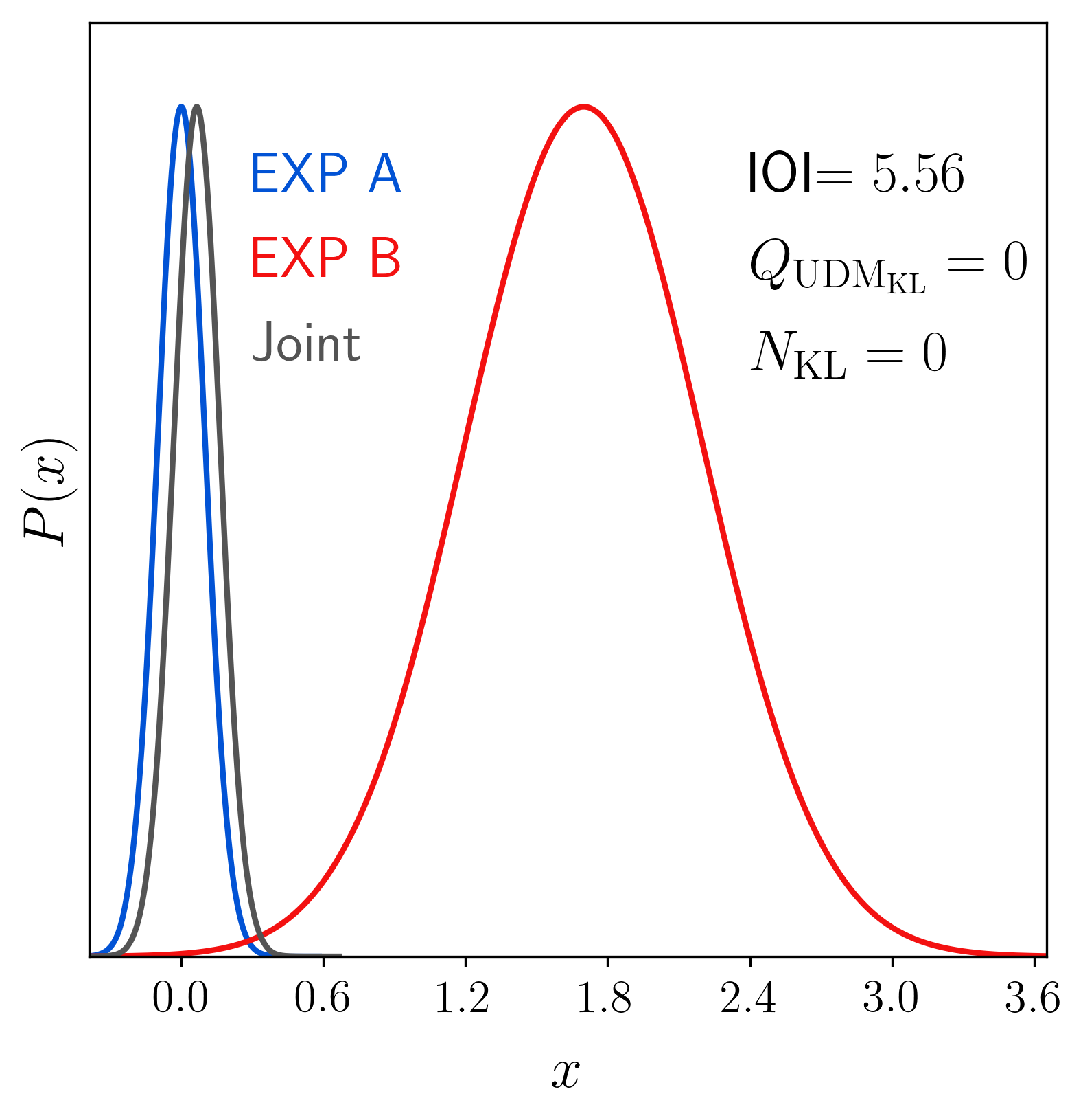
We provide here a numerical demonstration of this relationship in Fig. 1 as well as an exact analytical proof detailed in appendix A.
As we can observe in Fig. 1, after building two Gaussian distributions and obtaining the joint distribution, we can compute IOI for Exp A and Exp B, and compute by using Exp A and Joint. The Gaussian and weak prior limit refers to a situation where likelihoods are Gaussian on the parameters and the prior is weak.
To produce Fig. 1 and calculate the inconsistency measures, we proceed as follows. For the first toy-experiment (Exp A) we use
| (11) |
and
| (12) |
while for the second toy-experiment (Exp B), we set
| (13) |
and
| (14) |
The ellipses corresponding to the individual experiments are plotted, as well as that of the joint Gaussian analysis (gray). Then we calculate IOI and as given by the respective equations (1) and (4). The values obtained confirms the relationship (10) and the analytical proof of appendix A.
Finally, it is worth noting that IOI is a moment-based measure and requires distributions of model parameters to be nearly Gaussian. Therefore, when we want to perform a consistency analysis on two cosmological experiments whose parameter distributions are highly non-Gaussians, we need to combine them separately with other data in order to break degeneracies between parameters and to obtain Gaussian or nearly Gaussian distributions for the parameters. It is also worth pointing out that an advantage of IOI is that it can be applied to multiple experiments and data sets, and the multi-data set IOI has been applied to various multi-constraint comparisons in Ref. Lin and Ishak 2017b. Discussion of multiple experiments consistency comparisons is generally a subject not well covered in literature.
The measure works differently and can be applied to only two data sets at once. However,Ref. Raveri and Hu 2019 introduced as a measure that requires only one data set to provide a Gaussian parameter distribution, with no requirement of Gaussianty for the second data set, and that along with a KL decomposition it is numerically stable against non-Gaussianity. We will investigate the stability of both IOI and as well as the role of KL decomposition in section II.4.
Nonetheless, it is fair to assert that there are currently no perfect discordance measures that can be simultaneously applied to multiple data sets, cover non-Gaussian cases and accurately trace inconsistencies when they are present Lin and Ishak 2017a; March et al. 2011; Verde et al. 2013; MacCrann et al. 2015; Seehars et al. 2016; Grandis et al. 2016b; Joudaki et al. 2017; Raveri and Hu 2019; Adhikari and Huterer 2018; Handley and Lemos 2019.
II.4 Stability analysis
| Experiment 1 .vs. Experiment 2 | ||||||
|---|---|---|---|---|---|---|
| IOI | IOI | |||||
| TTTEEE + CMB lens .vs. DES + Added Probes | ||||||
| TTTEEE + CMB lens .vs. DES + Added Probes | ||||||
| TTTEEE + CMB lens .vs. DES + Added Probes | ||||||
| TTTEEE + CMB lens .vs. DES + Added Probes | ||||||
| TTTEEE + CMB lens .vs. DES + Added Probes | ||||||
| TTTEEE + CMB lens .vs. DES + Added Probes | ||||||
| TTTEEE + CMB lens .vs. DES + Added Probes | ||||||
| TTTEEE + CMB lens .vs. DES + Added Probes | ||||||
| TTTEEE + CMB lens .vs. DES + Added Probes | ||||||
| IOI | IOI | ||||
|---|---|---|---|---|---|
We run cosmological parameter estimation and inconsistency measure calculations (for IOI and ) using the same data sets multiple times. We analyze the values obtained and report standard deviations in each case as we discuss below. We use the CDM model with six cosmological parameters: and , the baryon and cold dark matter physical density parameters, respectively; , the ratio of the sound horizon to the angular diameter distance of the surface of last scattering multiplied by ; , the reionization optical depth; , the scalar-perturbation spectral index; and , the amplitude of the primordial power spectrum. In each MCMC sample for this section, we fix the reionization optical depth to 0.06 since it is not constrained by the other probes used. We compare Planck-2018 data against large-scale structure data from the Dark Energy Survey (DES) in combination with some added probes by calculating IOI, Q and Q. Specifically, we use the Planck CMB lensing measurements in combination with TT, TE, TT Planck high- temperature likelihood, used in Planck Collaboration et al. 2018a and described in Planck Collaboration et al. 2019. We label this combination as TTTEEE + CMB lens. On the other side, we use the clustering and lensing data from the DES Year 1 analysis Abbott and others DES Collaboration 2017 in combination with some added probes. We use BAO measurements from the BOSS Data Release 12 Alam et al. 2017, together with two BAO data sets from the 6DF Galaxy Survey Beutler et al. 2011 and the SDSS Data Release 7 Main Galaxy Sample Ross et al. 2015. We combine the BAO measurements with the supernova Pantheon compilation Scolnic et al. 2017 given by the combination of 279 Type Ia supernovae (SNe Ia) with useful distance estimates of SNe Ia from SDSS, SNLS, various low-z and HST samples, giving a total of 1048 SNe Ia ranging from . Additionally, we use BBN measurements from Cooke et al. 2017 in order to constrain , and we refer to this combination as DES + Added Probes. Finally, we obtain the constraints by using the publicly available Markov Chain Monte Carlo (MCMC) code CosmoMC Lewis and Bridle 2002.
We proceed as follows: we compare TTTEEE + CMB lens data against DES + AddedProbes. We run each data set a total of three times, so we can compare the two data sets a total of nine times. We label the first, second and third run of each experiment with , and , respectively. For a fixed convergence limit, a measure with a smaller standard deviation is more numerically stable. Furthermore, we do this process for two different chain convergence values, using a simple generalized Gelman-Rubin statistic Lewis 2013; Gelman and Rubin 1992, with values of and . Here, a value of is numerically more accurate than . Therefore, we expect a lower standard deviation for IOI and when is set to a lower value. Once we obtain the cosmological constraints, we compute IOI using equation (1), given by (4) and using (6). The results for each measure are compiled in Table 211 1 In this case, the relationship does not hold. Possible reasons for this might be the non-Gaussianity of the parameter distributions. We can also see that , this could be due to the removal of some noise-dominated modes in addition to the non-Gaussiantiy. Indeed, if we use distributions that are closer to Gaussian ones, such as the constraints from Planck and WMAP, the relation holds very well; see section III.2. Also holds very well too, since only one KL mode is removed. and the associated standard deviations divided by the mean values in Table 3.
As we can see in Table 2, IOI shows very similar values for each analysis. One can observe that this is consistently the case for the two convergence levels used. On the other hand, shows a much wider range of values with some of them being too large (e.g. for vs ), for the case of . We also obtain negative values (e.g. for vs ), which highlights some stability issues if used without KL decomposition. This instability in can be seen from equation (4). For Gaussian cases with no numerical noises, the factor is positive definite. But due to non-Gaussianity or just numerical noise, it is not the case anymore. The fact that is not positive definite in practice gives the possibilities of getting negative values of , which are difficult to interpret. This can be seen more clearly in KL modes; see our latter discussion. After the KL decomposition and filtering of modes associated with numerical noise are performed, becomes numerically stable. The KL decomposition decorrelates the modes and one then sorts the eigen-modes by order of improvement (i.e., by order of descending ). If the combined constraints only slightly improve the uncertainty on a particular KL mode compared to the first constraint, the corresponding will be closer to . The corresponding KL modes are numerically noisy and must be removed according to some threshold criterion. After removing the noisy modes (five modes for this case), one obtains with and it then becomes stable.
We express this dispersion by showing in Table 3 the standard deviation divided by the mean value associated with each measure of discordance. However, in the case of we do not consider the negative values, since they cannot be used to distinguish if an inconsistency is present. As shown there, has a large dispersion of and . After removing the noisy modes using the KL decomposition process, the standard deviations for are reduced to more acceptable values (i.e. and ) but they still remain more than twice the small values reached by IOI without any KL decomposition (i.e. and ).
In other words, we find that IOI has very stable values with very little dispersion. This is contrary to what was claimed in Raveri and Hu 2019 about measures of this type without any supporting specifications.
Finally, we show explicitly in what follows that the stability of IOI does not depend on the KL decomposition. Indeed, we can decorrelate the covariance matrices involved in the calculation of IOI (see Eq. (1)) by using an analogous modified eigenvalue problem to the one shown for in section II.2. We consider the modified eigenvalue problem as
| (15) |
where the covariance matrices are subject to the conditions
| (16) |
and
| (17) |
This leads to the following decorrelated form of IOI
| (18) |
where are the elements of the diagonal matrix and . In KL modes, both and are diagonalized.
A quick comparison between expressions (6) and (18) can tell us why IOI is stable by itself, while needs a removal process for noisy modes. In the case of the update difference in mean, we can have problems in two cases. The first case is that the factor is not always definite positive after MCMC sampling. This is because the eigenvalues can be smaller than , allowing for the possibility of a negative as seen in Table 2. The second case is when the first experiment has more constraining power than the second experiment in some particular modes. In this case the second experiment does not improve the constraint on a given mode much over the first one and this leads to . These modes can be identified after a KL transform and removed. Here, we remove the modes that satisfy the condition , where is the biggest mode. Note that this includes all modes with .
Now, in the case of IOI, two very similar experiments would lead to , but this would not drastically increase IOI. Moreover, if experiment 1 has more constraining power than experiment 2, this would lead to eigenmodes with . On the other hand, if experiment 2 is more constraining than experiment 1, we would observe some eigenmodes with . In any case, modes with would not affect (18) and would have negligible contributions. Finally, it is worth noting that the factor involved into the computation of IOI is always positive definite. Thus, the stability of IOI found numerically further above is confirmed analytically here.
III Parameter spaces, interpretation and KL decomposition
The interpretation of the measures of discordance is crucial in order to accurately represent the degree of inconsistency between cosmological data sets. Different approaches to interpret these measures have been discussed in the literature Handley and Lemos 2019; Charnock et al. 2017; Battye et al. 2015; Seehars et al. 2014; Marshall et al. 2006; Karpenka et al. 2015; Verde et al. 2013. A recent detailed discussion of the interpretation can be found in Lin and Ishak 2019 while we focus here on analyzing the question with respect to the decomposition of measures.
III.1 Interpretation of measures and KL mode-filtering algorithms

The interpretation of the values of IOI is done via Jeffreys’ scales. Jeffreys’s scales were empirical scales originally suggested for the interpretation of the Bayesian evidence ratio Jeffreys 1998. It was suggested in Lin and Ishak 2017a to use such scales for IOI because they matched well with the inconsistencies in the illustrative cases studied there and also some other measures that reduce or relate to IOI in Gaussian cases had used these Jeffreys’s scales Lin and Ishak 2017a. In that way, it was found practical to use the same scales to be able to compare these measures to one another. However, it worth noting that we use an overall more conservative terminology than in the original Jeffreys’s scales paper Jeffreys 1998 and similar to the one used in, for example, Ref. Trotta 2008 as shown in Table 1. Nonetheless, we point out that the category “moderate” in Table 1 does not mean “insignificant” or “ignorable”. On the contrary, one should understand “moderate” here as an indicator of a “non-ignorable” inconsistency. Finally, we provide a one-to-one relation between IOI and the commonly used confidence level of tension using the relation . One can observe then some agreement between Jeffrey’s scale and the n- language and the word “moderate” is, in fact, an indication of a non-ignorable inconsistency and in particular when IOI is in the high end of this range. The problem of significance and interpretation of inconsistency measures is a subject of ongoing debate in the literature and we refer the reader to discussions in for example Ref. Lin and Ishak 2019.
It was argued in Lin and Ishak 2019 that one should not use the conversion from IOI or a function of it to a probability to exceed (PTE) that depends on the number of parameters considered as for example done for . It was shown there that using higher parameter degrees of freedom in such a conversion results in underestimating inconsistencies.
Before we comment on the KL decomposition, we provide here an example to illustrate the argument presented in Lin and Ishak 2019. Let us consider a model with one parameter and let us assume that one experiment measures and , while a second experiment measures and . If we compute IOI using (1) we obtain IOI, this indicates a strong inconsistency that may be caused because of systematics in one of the experiments (or both), or problems with the underlying model. Another way to interpret this value is consider that IOI follows a -square distribution and compute , where represents the gamma function, while is the upper incomplete gamma function. For cases with only one parameter as here, the interpretation provided by this approach is suitable and is consistent with that of Jeffreys’ scales of IOI. Indeed, it will give us that which indicates a significant inconsistency. However, let us extent the model to a 10-parameters model where the first parameter follows the same distribution as before for both of the experiments, but the other 9 parameters show exactly the same distribution when they are measured by any of the two experiments. More specifically, the first experiment now measures and (diag means diagonal matrix), while the second experiment measures and . If this is the case, we would still obtain which according to the Jeffrey’s scale indicates a strong inconsistency, which is still given by the first parameter. However, since the number of degrees of freedom was increased by the addition of extra parameters, we obtain and the inconsistency is not significant anymore. Therefore, this example corroborates with Lin and Ishak 2019 and confirms that even in a case where we know that a given parameter shows a severe inconsistency, interpreting IOI using a PTE and significance level as describe above may lead to underestimate the inconsistency for a high dimensional parameter space.
Now, even though in many practical cases, the KL number of degrees of freedom appears to be small (1, 2 or even 0) for Raveri and Hu 2019, we show using illustrative constructions and a real data example that there exists cases where can remain large. A high value of may be explained by a significant improvement of constraint in each mode. But as we explained above, such a large can lead to underestimate an inconsistency when converted in terms of PTE and significance level. Right below are two illustrative numerical examples and a concrete example using real data from WMAP versus Planck is given in the next sub-section. In the three examples, this conversion leads to underestimation of inconsistencies.
We show in Fig. 2 an illustrative example where we can have as large as the original number of parameters with no reduction. Specifically, we consider a model given by the parameters and , which follow Gaussian distributions for both experiment A (Exp A) and experiment B (Exp B) as follows. For EXP A, the mean value is given by
| (19) |
while the associated covariance matrix is
| (20) |
Similarly, the mean value of EXP B is
| (21) |
and the covariance matrix of EXP B is the same that , then
| (22) |
Using Exp A and Exp B we can calculate the value of IOI to be 4.44. Additionally, we can obtain the joint distribution and compute , but even when we use the KL decomposition, Exp B offers a significant improvement on both modes so the algorithm for filtering modes after the KL decomposition does reduce . An exact similar example in which does not drop can be constructed in a higher parameter space. For such cases, the large will still affect the conversion to PTE which will underestimate the inconsistency.
Finally, it is important to mention that the KL decomposition process allows to analyze a measure of discordance in a more convenient basis. However, removing the numerical noise from a measure ultimately depends on the algorithm used to removes the noisy modes. The authors in Raveri and Hu 2019 presented an algorithm that allows to identify the numerical noise dominated modes. However, as they pointed out, if we combine a data set that is very constraining with a data set that weakly constrains the parameters, the algorithm used will drop all the modes, even when an inconsistency may be present. In Fig. 3 we show an illustrative example where two experiments present a strong inconsistency. Nevertheless, we can see that the algorithm for filtering modes after KL decomposition presented in Raveri and Hu 2019 will drop the parameter from the analysis, since its improvement is not big enough, even when an inconsistency was originally present.
On the other hand, we show in Fig. 3 that IOI can deal with such cases without requiring any further algorithm for filtering modes. This example shows a case where clearly IOI can properly trace an inconsistency with no need to discard valuable information via filtering mode algorithms. As we showed in section II.4 since, IOI is a stable measure of discordance with no need to mode filtering.
III.2 Are WMAP and Planck that consistent one with another? A case where does not reduce to a small number


 |
We recall that the number of degrees of freedom is usually reduced by the KL decomposition and the dropping of modes with numerical noise from MCMC sampling. The modes that are dominated by numerical noise come from comparing experiments where the second data set added does not improve much over the first data set (Gaussian), leading to (see section II.2). But this does not happen in all cases of interest as we discuss here.
Indeed, it is instructive to analyze IOI and in a situation where, even after the KL decomposition, the number of degrees of freedom remains high. For that, we compare WMAP9 which provides constraints with nearly Gaussian distribution for the base parameters against the full Planck-2018 data, which gives also Gaussian distributions for the parameters but with a higher constraining power.
We use the nine year results full WMAP data Hinshaw et al. 2013 and the full Planck-2018 data, TTTEEE high-, the low- polarization used in Planck Collaboration et al. 2018b and the CMB lensing measurements Planck Collaboration et al. 2018c in a joint analysis. Thus, we proceed by starting with WMAP data and then using the update procedure of using Planck data which should offer enough improvement over each mode so no decrease in is expected. We find that indeed, when six base cosmological parameters where considered (i.e. N=6). The analysis gives and after using the KL decomposition and removing the modes with numerical noise (in this case only one mode) we obtain .
Meanwhile, the comparison between WMAP and Planck gives IOI=3.29. Again, we can observe that because of the nearly Gaussian distributions of the parameters in both experiments we get .
Now, interpreting the value of IOI using the Jeffrey’s scale indicates a moderate inconsistency. On the other hand, interpreting using PTE leads to a non-significant inconsistency with for and for after removing one noise-dominated mode. However, this way of interpreting the results using PTE with a yet high number of degrees of freedom may underestimate the inconsistency as discussed in sub-section III.1 where we concur with the arguments of Ref. Lin and Ishak 2019.
Finally, in order to examine the tension found above by IOI, it is useful to analyze the constraints in a space where the parameters are not correlated. Therefore, we compare WMAP and Planck-2018 constraints by applying a change of basis using Eq. (15) and visualize the constraints when the parameters are decorrelated. Part of the results are shown in in Fig. 5 where we plot the two KL-modes that present the largest tensions. Among the six different modes, four of them are below the 1- level of tension. However, two modes present a tension of 1.4- and 2.1-. This can help one to see that even when there might not be a strong tension between WMAP and Planck-2018, the data sets are not as consistent as we may think from looking at the 1D marginalized contours. It is worth mentioning that other works have also pointed out some 3- tension present between WMAP and Planck-2015 data Larson et al. 2015; Hazra and Shafieloo 2014.
IV Application and results from current data sets
Combining data sets from different cosmological probes is crucial to disentangle the values of the cosmological parameters in a precise way. Also important is to jointly analyze data sets that are consistent with each other, in order to obtain reliable constraints. Therefore, after verifying the numerical stability of IOI, we apply it in order to trace inconsistencies between current data sets in this section. We compare CMB measurements from Planck-2018 against different Large-Scale-Structure (LSS) measurements in combination with some added probes. Additionally, we test the consistency between different measurements of the Hubble constant using IOI.
IV.1 Planck-2018 versus Large-Scale-Structure data sets
| Data sets | Description | Added probes |
| 1. Background | ||
| SH0ES | Locally measured Hubble constant Riess et al. 2019 | N/A |
| H0LiCOW | Strong gravitational lensing Wong et al. 2019 | N/A |
| CCHP-TGRB22 2 CCHP stands for Carnegie-Chicago Hubble Program | Tip of the Red Giant Branch (TRGB) applied to SNe Ia Freedman et al. 2019b | N/A |
| TRGB-2 | TRGB+SNe Ia distance ladder as re-analyzed with different methods by Yuan et al. 2019 | N/A |
| SNe | SNe Ia joint analysis data from Pantheon compilation Scolnic et al. 2017 | BBN33 3 Primordial deuterium abundance Cooke et al. 2017. |
| BAO | Six Degree Field Galactic Survey (6dF) () Beutler et al. 2011, SDSS main galaxy sample (MGS) () Ross et al. 2015 and BAO consensus constraints Alam et al. 2017 | BBN |
| 2. Planck-2018 temperature and polarization | ||
| TT+lowE | Planck high-44 4 High- represents the range . temperature auto correlation Planck Collaboration et al. 2018a | lowE55 5 Planck-2018 low- ( ) polarization Planck Collaboration et al. 2018a. Opposite to our previous work, here we only use the likelihood since a poor statistical consistency of the spectrum was reported in Planck Collaboration et al. 2018a. |
| TE+lowE | Planck high- temperature-E polarization cross correlation Planck Collaboration et al. 2018a | lowE |
| EE+lowE | Planck high- E-mode polarization auto correlation Planck Collaboration et al. 2018a | lowE |
| TTTEEE+lowE | Planck high- temperature and E-mode polarization joint data set Planck Collaboration et al. 2018a | lowE |
| 3. Large-Scale-Structure data sets | ||
| DES | Dark Energy Survey Year 1 clustering and lensing analysis Abbott and others DES Collaboration 2017 | lowE+SNe+BBN |
| CMB lens | Planck-2018 CMB lensing measurements Planck Collaboration et al. 2019 | lowE+SNe+BBN |
| SDSS RSD | SDSS III galaxy clustering data from BAO spectroscopic survey Alam et al. 2017 | lowE+SNe+BBN |
| Joint LSS | Joint analysis combining DES+CMB lens+SDSS RSD | lowE(or with priors)+BBN |
Inconsistencies between Planck and LSS have been pointed out in previous works Douspis et al. 2019; Kumar et al. 2019; Handley and Lemos 2019; Heymans et al. 2013; Hildebrandt et al. 2017; Blake et al. 2011; Lin and Ishak 2017b; Reid et al. 2014; Ade, P. A. R. et al (2016) Planck Collaboration; Planck Collaboration et al. 2018b. Here, we do a discordance/concordance analysis between the recently released Planck-2018 data against different LSS data sets using IOI.
We list the data sets used in this analysis in Table 4. In order to break denegeracies between some cosmological parameters and obtain Gaussian distribution for the parameters, we use some data sets as added probes in combination with the LSS measurements. However, we do this while taking care of not affect any inconsistency, if present, by such additions.
We consider three different data sets for LSS measurements. As we can see in Table 5, all data sets are consistent one with each other since IOI is less than the unity in each case. Moreover, the multi-experiment IOI is also less than unity when all LSS measurements are combined. Then, this allows us to combine them in a joint analysis as shown in section IV.2. However, it is important to mention that in order to get nearly Gaussian distributions for all the parameters, we use lowE+SNe+BBN as added probes. Similarly, we can repeat the same analysis for the internal consistency between Planck temperature and polarization measurements as shown in Table 6. In this case, we find that the values of IOI for TT+lowE when compared to TE+lowE or EE+lowE show an inconsistency in the high end of the weak range and close to 2.5. Furthermore, the values of IOI shows that a moderate inconsistency is present for TE+lowE and EE+lowE. Similarly, we find that the multi-experiment IOI shows a moderate inconsistency when combining the three data sets. Therefore, some moderate internal inconsistency is found in the Planck-2018 data indicating perhaps the presence of some systematic effects.
Next, we compare the Planck data against the LSS measurements after analyzing the self-consistency of Planck and LSS.The Planck temperature and polarization data shows a weak inconsistency with CMB lensing and SDSS RSD measurements. Therefore, we consider that combining these experiments in a joint analysis is fine, but we point out that further improvements need to be done in order to mitigate these small inconsistencies, even when they are weak inconsistencies. On the other hand, DES data shows a moderate inconsistency with TT+lowE, EE+lowE and TTTEEE+lowE data sets. This moderate inconsistency with DES seems similar to what was reported in Planck Collaboration et al. 2018b when including galaxy clustering data in DES data, as moderate percent-level tension. Additionally, we show that there is a moderate inconsistency between joint LSS and TE+lowE, as well as for EE+lowE. However, this inconsistency becomes a strong inconsistency when comparing joint LSS with TT+lowE or TTTEEE+lowE. Therefore, even when there is a weak inconsistency between Planck and CMB lens or SDSS RSD, or a moderate inconsistency with DES, combining the LSS probes in a joint analysis seriously increases the tension with Planck. It is important to mention that, the strong inconsistency between Planck and joint LSS should be attributed to LSS measurements and not BBN, since deuterium abundance determination Cooke et al. 2017 was found to be in no significant tension with Planck-2018 data Planck Collaboration et al. 2018b. Then, we point out that one should be aware of this tension when combining Planck and different LSS probes in a joint analysis.
It remains to be explored whether these inconsistencies are due to systematic effects in any of the data sets. However, we find that while SDSS RSD and CMB lensing show smaller inconsistencies with Planck-2018 (temperature and polarization data) which are lower with respect to what was found when comparing SDSS RSD and CMB lensing versus Planck-2015 in previous study Lin and Ishak 2017b. However, the inconsistency between weak lensing and Planck persist to be a moderate inconsistency, according to Table 1. Finally, the inconsistency with a joint analysis of this LSS probes and Planck is a strong inconsistency with IOI=5.27.
| CMB lens | DES | SDSS RSD | |
|---|---|---|---|
| CMB lens | - | 0.41 | 0.75 |
| DES | 0.41 | - | 0.81 |
| SDSS RSD | 0.75 | 0.81 | - |
| Multiexperiment IOI = 0.74 | |||
| Planck | TT+lowE | TE+lowE | EE+lowE |
|---|---|---|---|
| TT+lowE | - | 2.43 | 2.45 |
| TE+lowE | 2.43 | - | 3.19 |
| EE+lowE | 2.45 | 3.19 | - |
| Multiexperiment IOI = 3.39 | |||
| CMB lens | DES | SDSS RSD | Joint LSS | |
|---|---|---|---|---|
| TT+lowE | 1.83 | 3.28 | 0.90 | 5.01 |
| TE+lowE | 1.54 | 1.54 | 0.40 | 3.90 |
| EE+lowE | 2.07 | 3.13 | 1.39 | 3.97 |
| TTTEEE+lowE | 1.60 | 3.14 | 0.70 | 5.27 |
IV.2 Consistency analysis of the Hubble constant from various data sets

| Planck | SH0ES | Joint LSS (with priors) | H0LiCOW | SNe+BAO +BBN | CCHP-TRGB | TRGB-2 | |
|---|---|---|---|---|---|---|---|
| Planck | 9.70 | 0.04 | 5.25 | 0.36 | 0.75 | 3.24 | |
| SH0ES66 6 We consider SH0ES, CCHP-TRGB and TRGB-2 as representing the same probe. | 9.70 | 6.73 | 0.05 | 2.68 | 1.59 | 0.24 | |
| Joint LSS | 0.04 | 6.73 | 3.89 | 0.18 | 0.48 | 2.41 | |
| H0LiCOW | 5.25 | 0.05 | 3.89 | 1.63 | 0.92 | 0.06 | |
| SNe+BAO+BBN | 0.36 | 2.68 | 0.18 | 1.63 | 0.06 | 0.94 | |
| CCHP-TRGBa | 0.75 | 1.59 | 0.48 | 0.92 | 0.06 | 0.47 | |
| TRGB-2a | 3.24 | 0.24 | 2.41 | 0.06 | 0.94 | 0.47 |
| Data sets | All | Removing Planck | Removing SH0ES | Removing joint LSS (with priors) | Removing H0LiCOW | Removing SNe+BAO+BBN |
|---|---|---|---|---|---|---|
| Mutiexperiment IOI | 5.63 | 4.38 | 2.73 | 6.90 | 4.94 | 7.01 |
The clear tension reported in the Hubble constant between the local measurement and the CMB inferred value has generated a lot of discussions and comparison, see for example the partial list Riess et al. 2019; Vagnozzi 2019; Lin et al. 2019; Desmond et al. 2019; Poulin et al. 2018; Graef et al. 2019; El-Zant et al. 2019; Carneiro et al. 2019; Kreisch et al. 2019; Prilepina and Tsai 2017; Zhao et al. 2017; Feng et al. 2017; Dirian 2017; Di Valentino et al. 2017; Solà et al. 2017; Khosravi et al. 2019; Bolejko 2018; Bernal et al. 2016a; Di Valentino et al. 2016. In our previous work, we presented five different methods to constraint Lin and Ishak 2017b. Here, we update the analysis with current new data sets and the way we combine them.
We use the data sets presented in Table 4 to compare different measurements from 1) Planck: CMB measurements using Planck-2018 data, specifically we use the measurement TTTEEE+lowE+CMB lens used in Planck Collaboration et al. 2018b; 2) SH0ES: Local measurements of from Riess et al. 2019; 3) Joint LSS: Joint analysis using three distinct LSS measurements as in Table 4 77 7 In addition, we add BBN in order to break the degeneracy in .; 4) SNe+BAO+BBN: Combination of background data sets to constraint . SNe and BAO have different degeneracy directions, while BBN can constraint ; 5) H0LiCOW: measures expansion rate of the universe using time-delay cosmography and distance ladder results Wong et al. 2019; 6) CCHP-TRGB: Calibration of SNe Ia using the TRGB method, independent of the Cepheid distance scale Freedman et al. 2019b; 7) TRGB-2: TRGB+SNe Ia distance ladder using a different calibration method Yuan et al. 2019. The values of obtained from each of these methods are given in Fig. 6.
We report the values of IOI for all the combinations of the seven data sets in Table 8. We can see that the biggest inconsistency is obtained when comparing Planck against SH0ES measurements, leading to a value of IOI=9.70 which is a strong inconsistency. In one dimension (one parameter), we can convert this IOI value to the commonly used confidence level of tension by using -. Then, we obtain a tension between Planck-2018 and SH0ES measurements of -. This is exactly what was reported in Riess et al. 2019. Similarly, Planck and H0LiCOW indicate a strong inconsistency with IOI higher than 5. Here, it is worth mentioning that SH0ES and H0LiCOW measurements are consistent one with each other with a value of IOI=0.05. Therefore, both data sets can be jointly analyzed. A previous work reported that by combining SH0ES and H0LiCOW data sets in a joint analysis gives km s-1Mpc-1 Wong et al. 2019, producing a tension of 5.3- with Planck. In our case, we obtain IOI=14.03 if we compare H0LiCOW+SH0ES against Planck. This is equivalent to the 5.3- level of tension mentioned before. Similarly, a strong inconsistency is present between joint LSS and late universe probes H0LiCOW+SH0ES with IOI=8.59, equivalent to a 4.1- level of tension.
We find that joint LSS presents a strong inconsistency with SH0ES and a moderate inconsistency with H0LiCOW, which can be translated to a tension of 3.7- and 2.8-, respectively. Furthermore, SNe+BAO+BBN presents a moderate inconsistency with SH0ES but a weak inconsistency with H0LiCOW. On the other hand, Planck seems to be consistent with joint LSS and SNe+BAO+BBN, while these two data sets are actually consistent one with another.
The recent Hubble constant measurement obtained by Freedman et al. 2019b using the Tip of the Red Giant Branch is midway and in overall consistent with both SH0ES and Planck, with only an IOI of 1.59 with SH0ES (1.78-) and an IOI of 0.75 1.23- with Planck, again in agreement with the values reported in Freedman et al. 2019b. Ref. Yuan et al. 2019 redid the TRGB analysis using other correction/calibration methods and found a higher value of , still in some tension with Planck.
We also compute the multi-experiment IOI values using Eq. (3) in Table 8. Comparing all data sets leads to values of IOI, which stands for a strong inconsistency according to Table 1. We remove alternatively some data sets and see how the inconsistency drops. This value goes higher if we remove SNe+BAO+BBN or joint LSS , making the inconsistency more severe. This is because 1) these data sets are consistent one with another, and 2) these data sets are consistent with Planck. On the other hand, the value of the multi-experiment IOI drops if we remove Planck, H0LiCOW or SH0ES measurements. Indeed, removing these data sets reduce the inconsistency to a moderate inconsistency.
Noteworthy is that we find here a new strong tension between SH0ES and that of joint LSS probes with IOI=6.73 corresponding in 1D to 3.7-.
V Summary and concluding remarks
First, we studied some properties of recently proposed parameter-distance based measures of inconsistencies. Namely the index of inconsistency (IOI) of Ref. Lin and Ishak 2017a and the updated measure () of Ref. Raveri and Hu 2019. We showed that in the nearly Gaussian cosmological parameter distributions and weak prior limit, the two measures are equal, up to a factor 2, i.e. . A Karhunen-Loeve (KL) decomposition was applied to in Raveri and Hu 2019 in order to eliminate modes with numerical noise for the quantity. We showed that IOI does not need such a decomposition.
Importantly, we investigate the question of stability by repeating cosmological and consistency analyses using the two measures, imposing two convergence limits, and reporting the mean values and standard deviations of the results obtained. We find that IOI gives a small relative standard deviation of which indicates high stability. gives a relative standard deviation of without the KL decomposition and after such a decomposition. It is thus found here that IOI gives a better standard deviation than with or without KL decomposition. Our finding was also confirmed by an analytical result using KL decomposition.
Next, we discussed the question of interpretation of these inconsistency measures and the effect of the KL decomposition and its mode-filtering algorithms. It was argued in a recent analysis Lin and Ishak 2019 that the procedure of translating the values of IOI or into probability to exceed and significance level in high dimensional (parameter) spaces can underestimate inconsistencies due to high number of parameters or degrees of freedom. It was explain there that while such a procedure is justified when performing data fitting, importing it to the interpretation levels of inconsistency measures may not be the case.
Specifically, we showed here that while the KL decomposition in general transforms the degree of freedom from to which is much smaller than , this is not always the case. We provided an illustrative construction where stays the same and also showed that in the case of WMAP updated by Planck it decreases from to . So the effect of underestimating inconsistency may still happen here.
An example was also provided where the mode-filtering algorithm used with the KL decomposition discards a mode that contains a significant inconsistency and thus misses it.
In a second part of the paper, we perform various consistency analyzes using IOI between current multiple data sets and working within the entire parameter spaces.
We find current LSS data sets (CMB lensing from Planck-2018, DES Y1 and SDSS RSD DR12) to be all consistent one with another with IOI less than 1. This is not the case for Planck temperature (TT) vs polarization (TE,EE) data where moderate inconsistencies are present, particularly between TE+lowE and EE+lowE with IOI=3.19 and when all combined with IOI=3.39. Moderate inconsistencies are also found for Planck-2018 versus DES-Y1 with IOI=3.28. Such an inconsistency reaches the strong range when comparing Planck versus joint LSS probes with IOI=5.01 and IOI=5.27 when using TT+lowE and TTTEEE+lowE, respectively. Our results thus indicate that moderate and non-ignorable tensions are present between Planck and LSS when the whole parameter spaces are compared. This is in agreement with previous studies that focused on marginalized constraints on or such as in Refs. Wibking et al. 2019; Dossett et al. 2015; Joudaki et al. 2019. Unlike previous results in Lin and Ishak 2017b; Raveri and Hu 2019 using Planck-2015, we find here that CMB lensing has only weak inconsistencies with CMB temperature and polarization data from Planck-2018.
Finally, we provided a consistency study of the Hubble constant as determined from seven data sets. We find and confirm a strong inconsistency between the local measurement from SH0ES (LMH) versus Planck-2018 with IOI=9.70 (i.e. 4.40- in this 1D case) and concurring with Riess et al. 2019. Next, H0LiCOW versus Planck gives IOI=5.25 (3.24-). Moreover, since LMH and H0LiCOW are consistent one with another (IOI=0.05), we can combine them and compare them to Planck. We find that H0LiCOW+LMH versus Planck gives IOI=14.03 (i.e. 5.30-) which is substantial and in agreement with Wong et al. 2019. We also compared the constraints from CCHP-TRGB with other data sets and find them to be in overall consistency with SH0ES and Planck as reported in Freedman et al. 2019a.
We find that joint LSS data sets (CMB lensing + DES + SDSS RSD) versus SH0ES LMH shows a new strong tension of IOI=6.73 (i.e. 3.7-). Similarly, a strong inconsistency is found between joint LSS and late universe probes H0LiCOW+SH0ES with IOI=8.59, equivalent to a 4.1- level of tension.
The tensions discussed above are not fading away. Whether they are due to systematic effects in the data sets or the manifestation of problems with the underlying model, the causes of these old and new tensions need to be identified and addressed.
Acknowledgements.
The authors thank Adam Riess for useful comments on the manuscript. MI acknowledges that this material is based upon work supported in part by the U.S. Department of Energy, Office of Science, under Award Number DE-SC0019206 and the National Science Foundation under grant AST-1517768. CGQ gratefully acknowledges a PhD scholarship from the Mexican National Council for Science and Technology (CONACYT). The authors acknowledge the Texas Advanced Computing Center (TACC) at The University of Texas at Austin for providing HPC resources that have contributed to the research results reported within this paper. URL: http://www.tacc.utexas.edu.Appendix A Proof for in the Gaussian and weak prior limit
We have shown different situations where or, using real data, that . However, as mentioned, this relation holds in the Gaussian and weak prior limit. Then, we proof that can be derived from IOI in such a limit. Indeed, in general the joint mean value given data sets 1 and 2, is given by
| (23) |
and the joint covariance matrix can be obtained by
| (24) |
where is the prior covariance matrix and is the prior mean value.
Now, since IOI is designed to work with Gaussian data sets we assume we are working with Gaussian distributions. Moreover, we use a weak prior limit approximation by considering . Under these assumptions, (23) and (24) can be written as
| (25) |
and
| (26) |
respectively. Then, by using matrix properties we can show that
| (27) |
Then, we can write the difference of the mean value of the first data set and the mean value of the joint analysis as
| (28) |
Similarly, we can rewrite the difference between the covariance matrix of the first data set and the joint covariance matrix as
| (29) |
References
- Riess et al. (2019) A. G. Riess, S. Casertano, W. Yuan, L. Macri, and D. Scolnic, Astrophys. J. 07603 (2019), eprint 1903.07603.
- Poulin et al. (2019) V. Poulin, T. L. Smith, T. Karwal, and M. Kamionkowski, Phys. Rev. Lett. 122, 221301 (2019).
- Efstathiou (2014) G. Efstathiou, Mon. Not. R. Astron. Soc. 440, 1138 (2014), eprint 1311.3461.
- Freedman et al. (2019a) W. L. Freedman, B. F. Madore, D. Hatt, T. J. Hoyt, I. S. Jang, R. L. Beaton, C. R. Burns, M. G. Lee, A. J. Monson, J. R. Neeley, et al., Astrophys. J. 882, 34 (2019a), eprint 1907.05922.
- Yuan et al. (2019) W. Yuan, A. G. Riess, L. M. Macri, S. Casertano, and D. Scolnic, arXiv e-prints arXiv:1908.00993 (2019), eprint 1908.00993.
- Arendse et al. (2019) N. Arendse, R. J. Wojtak, A. Agnello, G. C. F. Chen, C. D. Fassnacht, D. Sluse, S. Hilbert, M. Millon, V. Bonvin, K. C. Wong, et al., arXiv e-prints arXiv:1909.07986 (2019), eprint 1909.07986.
- Knox and Millea (2019) L. Knox and M. Millea, arXiv e-prints arXiv:1908.03663 (2019), eprint 1908.03663.
- Davis et al. (2019) T. M. Davis, S. R. Hinton, C. Howlett, and J. Calcino, arXiv e-prints arXiv:1907.12639 (2019), eprint 1907.12639.
- Di Valentino et al. (2016) E. Di Valentino, A. Melchiorri, and J. Silk, Physics Letters B 761, 242 (2016), eprint 1606.00634.
- Kenworthy et al. (2019) W. D. Kenworthy, D. Scolnic, and A. Riess, Astrophys. J. 875, 145 (2019), eprint 1901.08681.
- Pustilnik et al. (2019) S. A. Pustilnik, A. L. Tepliakova, and D. I. Makarov, Mon. Not. R. Astron. Soc. 482, 4329 (2019).
- Verde et al. (2019) L. Verde, T. Treu, and A. G. Riess, arXiv e-prints arXiv:1907.10625 (2019), eprint 1907.10625.
- Blinov et al. (2019) N. Blinov, K. J. Kelly, G. Krnjaic, and S. D. McDermott, arXiv e-prints arXiv:1905.02727 (2019), eprint 1905.02727.
- Vagnozzi (2019) S. Vagnozzi, ArXiv e-prints (2019), eprint 1907.07569.
- Lin et al. (2019) M.-X. Lin, G. Benevento, W. Hu, and M. Raveri, arXiv e-prints arXiv:1905.12618 (2019), eprint 1905.12618.
- Desmond et al. (2019) H. Desmond, B. Jain, and J. Sakstein, arXiv e-prints arXiv:1907.03778 (2019), eprint 1907.03778.
- Poulin et al. (2018) V. Poulin, K. K. Boddy, S. Bird, and M. Kamionkowski, Phys. Rev. D 97, 123504 (2018), eprint 1803.02474.
- Graef et al. (2019) L. L. Graef, M. Benetti, and J. S. Alcaniz, Phys. Rev. D 99, 043519 (2019), eprint 1809.04501.
- El-Zant et al. (2019) A. El-Zant, W. El Hanafy, and S. Elgammal, Astrophys. J. 871, 210 (2019), eprint 1809.09390.
- Carneiro et al. (2019) S. Carneiro, P. C. de Holanda, C. Pigozzo, and F. Sobreira, Phys. Rev. D 100, 023505 (2019), eprint 1812.06064.
- Kreisch et al. (2019) C. D. Kreisch, F.-Y. Cyr-Racine, and O. Doré, arXiv e-prints arXiv:1902.00534 (2019), eprint 1902.00534.
- Prilepina and Tsai (2017) V. Prilepina and Y. Tsai, Journal of High Energy Physics 2017, 33 (2017), eprint 1611.05879.
- Zhao et al. (2017) G.-B. Zhao et al., Nature Astronomy 1, 627 (2017), eprint 1701.08165.
- Feng et al. (2017) L. Feng, J.-F. Zhang, and X. Zhang, European Physical Journal C 77, 418 (2017), eprint 1703.04884.
- Dirian (2017) Y. Dirian, Phys. Rev. D 96, 083513 (2017), eprint 1704.04075.
- Di Valentino et al. (2017) E. Di Valentino, A. Melchiorri, and O. Mena, Phys. Rev. D 96, 043503 (2017), eprint 1704.08342.
- Solà et al. (2017) J. Solà, A. Gómez-Valent, and J. de Cruz Pérez, Physics Letters B 774, 317 (2017), eprint 1705.06723.
- Khosravi et al. (2019) N. Khosravi, S. Baghram, N. Afshordi, and N. Altamirano, Phys. Rev. D 99, 103526 (2019), eprint 1710.09366.
- Bolejko (2018) K. Bolejko, Phys. Rev. D 97, 103529 (2018), eprint 1712.02967.
- Bernal et al. (2016a) J. L. Bernal, L. Verde, and A. G. Riess, J. Cosmol. Astropart. Phys. 10, 019 (2016a), eprint 1607.05617.
- Wibking et al. (2019) B. D. Wibking, D. H. Weinberg, A. N. Salcedo, H.-Y. Wu, S. Singh, S. Rodríguez-Torres, L. H. Garrison, and D. J. Eisenstein, arXiv e-prints arXiv:1907.06293 (2019), eprint 1907.06293.
- Joudaki et al. (2019) S. Joudaki, H. Hildebrandt, D. Traykova, N. E. Chisari, C. Heymans, A. Kannawadi, K. Kuijken, A. H. Wright, M. Asgari, T. Erben, et al., arXiv e-prints arXiv:1906.09262 (2019), eprint 1906.09262.
- Blake et al. (2011) C. Blake et al., Mon. Not. R. Astron. Soc. 415, 2876 (2011), eprint 1104.2948.
- Lange et al. (2019) J. U. Lange, X. Yang, H. Guo, W. Luo, and F. C. van den Bosch, Monthly Notices of the Royal Astronomical Society 488, 5771 (2019), ISSN 0035-8711, eprint http://oup.prod.sis.lan/mnras/article-pdf/488/4/5771/29190717/stz2124.pdf, URL https://doi.org/10.1093/mnras/stz2124.
- Bernal et al. (2016b) J. L. Bernal, L. Verde, and A. J. Cuesta, J. Cosmol. Astropart. Phys. 2, 059 (2016b), eprint 1511.03049.
- Reid et al. (2014) B. A. Reid, H.-J. Seo, A. Leauthaud, J. L. Tinker, and M. White, Mon. Not. R. Astron. Soc. 444, 476 (2014), eprint 1404.3742.
- Ade, P. A. R. et al (2016) (Planck Collaboration) Ade, P. A. R. et al (Planck Collaboration), Astron. Astrophys. 594, A24 (2016), eprint 1502.01597.
- Vikhlinin et al. (2009) A. Vikhlinin et al., Astrophys. J. 692, 1060 (2009), eprint 0812.2720.
- Di Valentino et al. (2019) E. Di Valentino, A. Melchiorri, O. Mena, and S. Vagnozzi, arXiv e-prints arXiv:1908.04281 (2019), eprint 1908.04281.
- Lin and Ishak (2017a) W. Lin and M. Ishak, Phys. Rev. D 96, 023532 (2017a), eprint 1705.05303.
- Hildebrandt et al. (2017) H. Hildebrandt et al., Mon. Not. R. Astron. Soc. 465, 1454 (2017), eprint 1606.05338.
- Lin and Ishak (2017b) W. Lin and M. Ishak, Phys. Rev. D 96, 083532 (2017b), eprint 1708.09813.
- Handley and Lemos (2019) W. Handley and P. Lemos, Phys. Rev. D 100, 043504 (2019), eprint 1902.04029.
- Ruiz and Huterer (2015) E. J. Ruiz and D. Huterer, Phys. Rev. D 91, 063009 (2015), eprint 1410.5832.
- Bridle and King (2007) S. Bridle and L. King, New Journal of Physics 9, 444 (2007), eprint 0705.0166.
- Krause et al. (2016) E. Krause, T. Eifler, and J. Blazek, Mon. Not. R. Astron. Soc. 456, 207 (2016), eprint 1506.08730.
- Yao et al. (2017) J. Yao, M. Ishak, W. Lin, and M. Troxel, J. Cosmol. Astropart. Phys. 2017, 056 (2017), eprint 1707.01072.
- Ishak et al. (2006) M. Ishak, A. Upadhye, and D. N. Spergel, Phys. Rev. D 74, 043513 (2006).
- Clifton et al. (2012) T. Clifton, P. G. Ferreira, A. Padilla, and C. Skordis, Phys. Rep. 513, 1 (2012), eprint 1106.2476.
- Koyama (2016) K. Koyama, Rep. Progr. Phys. 79, 046902 (2016), eprint 1504.04623.
- Joyce et al. (2015) A. Joyce, B. Jain, J. Khoury, and M. Trodden, Phys. Rep. 568, 1 (2015), eprint 1407.0059.
- Joyce et al. (2016) A. Joyce, L. Lombriser, and F. Schmidt, Annu. Rev. Nucl. Part. Sci. 66, 95 (2016), eprint 1601.06133.
- Ishak (2019) M. Ishak, Living Reviews in Relativity 22, 1 (2019), eprint 1806.10122.
- Stephani et al. (2003) H. Stephani, D. Kramer, M. A. H. MacCallum, C. Hoenselaers, and E. Herlt, Exact solutions of Einstein’s field equations, Cambridge Monographs on Mathematical Physics (Cambridge Univ. Press, Cambridge, 2003), ISBN 9780521467025, 0521467020, 9780511059179, 9780521467025, URL http://www.cambridge.org/uk/catalogue/catalogue.asp?isbn=0521461367.
- Bolejko (2011) K. Bolejko, J. Cosmol. Astropart. Phys. 2011, 025 (2011), eprint 1101.3338.
- Ishak and Peel (2012) M. Ishak and A. Peel, Phys. Rev. D 85, 083502 (2012), eprint 1104.2590.
- Peel et al. (2014) A. Peel, M. A. Troxel, and M. Ishak, Phys. Rev. D 90, 123536 (2014), eprint 1408.4390.
- Marshall et al. (2006) P. Marshall, N. Rajguru, and A. Slosar, Phys. Rev. D 73, 067302 (2006), eprint astro-ph/0412535.
- March et al. (2011) M. C. March, R. Trotta, L. Amendola, and D. Huterer, Mon. Not. R. Astron. Soc. 415, 143 (2011), eprint 1101.1521.
- Verde et al. (2013) L. Verde, P. Protopapas, and R. Jimenez, Physics of the Dark Universe 2, 166 (2013), eprint 1306.6766.
- MacCrann et al. (2015) N. MacCrann, J. Zuntz, S. Bridle, B. Jain, and M. R. Becker, Mon. Not. R. Astron. Soc. 451, 2877 (2015), eprint 1408.4742.
- Battye et al. (2015) R. A. Battye, T. Charnock, and A. Moss, Phys. Rev. D 91, 103508 (2015), eprint 1409.2769.
- Charnock et al. (2017) T. Charnock, R. A. Battye, and A. Moss, Phys. Rev. D 95, 123535 (2017), eprint 1703.05959.
- Seehars et al. (2014) S. Seehars, A. Amara, A. Refregier, A. Paranjape, and J. Akeret, Phys. Rev. D 90, 023533 (2014), eprint 1402.3593.
- Seehars et al. (2016) S. Seehars, S. Grandis, A. Amara, and A. Refregier, Phys. Rev. D 93, 103507 (2016), eprint 1510.08483.
- Grandis et al. (2016a) S. Grandis, S. Seehars, A. Refregier, A. Amara, and A. Nicola, J. Cosmol. Astropart. Phys. 5, 034 (2016a), eprint 1510.06422.
- Joudaki et al. (2017) S. Joudaki et al., Mon. Not. R. Astron. Soc. 465, 2033 (2017), eprint 1601.05786.
- Adhikari and Huterer (2018) S. Adhikari and D. Huterer, ArXiv e-prints (2018), eprint 1806.04292.
- Raveri and Hu (2019) M. Raveri and W. Hu, Phys. Rev. D 99, 043506 (2019), eprint 1806.04649.
- Park and Rozo (2019) Y. Park and E. Rozo, arXiv e-prints arXiv:1907.05798 (2019), eprint 1907.05798.
- Nicola et al. (2019) A. Nicola, A. Amara, and A. Refregier, J. Cosmol. Astropart. Phys. 2019, 011 (2019), eprint 1809.07333.
- Köhlinger et al. (2019) F. Köhlinger, B. Joachimi, M. Asgari, M. Viola, S. Joudaki, and T. Tröster, Mon. Not. R. Astron. Soc. 484, 3126 (2019), eprint 1809.01406.
- Karhunen (1947) K. Karhunen, Ann. Acad. Sci. Fennicae. Ser. A. I. Math.-Phys (1947).
- Loeve (1978) M. Loeve, Springer-Verlag. ISBN 0-387-90262-7. (1978).
- Tegmark et al. (2018) M. Tegmark, A. Taylor, and A. Heavens, Astrophys. J. 480, 22 (2018), eprint 9603021.
- Pacaud et al. (2018) F. Pacaud et al., Astron. Astrophys. p. 620 (2018), eprint 1810.01624.
- Camarena and Marra (2018) D. Camarena and V. Marra, Phys. Rev. D. D98, 023537 (2018), eprint 1805.09900.
- Camarena and Marra (2019) D. Camarena and V. Marra, ArXiv e-prints (2019), eprint 1906.11814.
- Lin and Ishak (2019) W. Lin and M. Ishak, arXiv e-prints arXiv:1909.10991 (2019), eprint 1909.10991.
- Handley and Lemos (2019) W. Handley and P. Lemos, Phys. Rev. D 100, 043504 (2019), eprint 1902.04029.
- Jeffreys (1998) H. Jeffreys, The Theory of Probability, Oxford Classic Texts in the Physical Sciences (OUP Oxford, 1998), ISBN 9780191589676.
- Grandis et al. (2016b) S. Grandis, D. Rapetti, A. Saro, J. J. Mohr, and J. P. Dietrich, Mon. Not. R. Astron. Soc. 463, 1416 (2016b), eprint 1604.06463.
- Planck Collaboration et al. (2018a) Planck Collaboration, N. Aghanim, et al., ArXiv e-prints (2018a), eprint 1807.06209.
- Planck Collaboration et al. (2019) Planck Collaboration, N. Aghanim, et al., ArXiv e-prints (2019), eprint 1907.12875.
- Abbott and others DES Collaboration (2017) T. M. C. Abbott and others DES Collaboration, ArXiv e-prints (2017), eprint 1708.01530.
- Alam et al. (2017) S. Alam, M. Ata, S. Bailey, et al., Mon. Not. R. Astron. Soc. 470, 2617 (2017), eprint 1607.03155.
- Beutler et al. (2011) F. Beutler, C. Blake, M. Colless, D. H. Jones, L. Staveley-Smith, L. Campbell, Q. Parker, W. Saunders, and F. Watson, Mon. Not. R. Astron. Soc. 416, 3017 (2011), eprint 1106.3366.
- Ross et al. (2015) A. J. Ross, L. Samushia, C. Howlett, W. J. Percival, A. Burden, and M. Manera, Mon. Not. R. Astron. Soc. 449, 835 (2015), eprint 1409.3242.
- Scolnic et al. (2017) D. M. Scolnic, D. O. Jones, A. Rest, et al., ArXiv e-prints (2017), eprint 1710.00845.
- Cooke et al. (2017) R. Cooke et al., Astrophys. J. 855, aaab53 (2017), eprint 1710.11129.
- Lewis and Bridle (2002) A. Lewis and S. Bridle, Phys. Rev. D 66, 103511 (2002), eprint astro-ph/0205436.
- Lewis (2013) A. Lewis, Phys. Rev. D 87, 103529 (2013), eprint 1304.4473.
- Gelman and Rubin (1992) A. Gelman and D. Rubin, Statistical Science 7, 457 (1992), eprint http://www.stat.columbia.edu/ gelman/research/published/itsim.pdf.
- Karpenka et al. (2015) N. V. Karpenka, F. Feroz, and M. P. Hobson, Mon. Not. R. Astron. Soc. 449, 2405 (2015), eprint 1407.5496.
- Trotta (2008) R. Trotta, Contemporary Physics 49, 71 (2008), eprint 0803.4089.
- Hinshaw et al. (2013) G. Hinshaw et al., Astrophys. J. Supp. 208, 19 (2013), eprint 1212.5226.
- Planck Collaboration et al. (2018b) Planck Collaboration, N. Aghanim, Y. Akrami, M. Ashdown, J. Aumont, C. Baccigalupi, M. Ballardini, A. J. Banday, R. B. Barreiro, and N. Bartolo, arXiv e-prints arXiv:1807.06209 (2018b), eprint 1807.06209.
- Planck Collaboration et al. (2018c) Planck Collaboration, N. Aghanim, et al., arXiv e-prints 06210 (2018c), eprint 1807.06210.
- Larson et al. (2015) D. Larson, J. L. Weiland, G. Hinshaw, and C. L. Bennett, Astrophys. J. 801, 9 (2015), eprint 1409.7718.
- Hazra and Shafieloo (2014) D. K. Hazra and A. Shafieloo, Phys. Rev. D 89, 043004 (2014), eprint 1308.2911.
- Wong et al. (2019) K. C. Wong et al., Mon. Not. R. Astron. Soc. (2019), eprint 1907.04869.
- Freedman et al. (2019b) W. L. Freedman, B. F. Madore, D. Hatt, T. J. Hoyt, I. S. Jang, R. L. Beaton, C. R. Burns, M. G. Lee, A. J. Monson, J. R. Neeley, et al., Astrophys. J. 882, 34 (2019b), eprint 1907.05922.
- Douspis et al. (2019) M. Douspis, L. Salvati, and N. Aghanim, arXiv e-prints arXiv:1901.05289 (2019), eprint 1901.05289.
- Kumar et al. (2019) S. Kumar, R. C. Nunes, and S. K. Yadav, European Physical Journal C 79, 576 (2019), eprint 1903.04865.
- Heymans et al. (2013) C. Heymans et al., Mon. Not. R. Astron. Soc. 432, 2433 (2013), eprint 1303.1808.
- Dossett et al. (2015) J. N. Dossett, M. Ishak, D. Parkinson, and T. M. Davis, Phys. Rev. D 92, 023003 (2015), eprint 1501.03119.