A simple model of Keratocyte membrane dynamics Preprint: APS/123-QED

Mohammad Abu Hamed Affiliation: Department of Mathematics, Technion - Israel Institute of Technology, Haifa 32000, Israel Affiliation: Department of Mathematics, Al-Qasemi, Academic College Of Education, Baqa El-Garbiah 30100, Israel Affiliation: Department of Mathematics, The College of Sakhnin - Academic College for Teacher Education, Sakhnin 30810, Israel Alexander A. Nepomnyashchy Affiliation: Department of Mathematics, Technion - Israel Institute of Technology, Haifa 32000, Israel

Abstract

We perform an analytical investigation of the cell interface dynamics in the framework of a minimal phase field model of cell motility suggested in Ziebert et al. 2012, which consists of two coupled evolution equations for the order parameter and a two-dimensional vector field describing the actin network polarization (orientation). We derive a closed evolutionary integro-differential equation governing the cell interface dynamics. The equation includes the normal velocity of the membrane, curvature, volume relaxation, and a parameter that is determined by the non-equilibrium effects in the cytoskeleton. This equation can be simplified to obtain a Burgers-like equation. A condition on the system parameters for the existence of a stationary cell shape is obtained.

I Introduction

Understanding the mechanics of cell motility is needed for design of artificial cells Kendall 2018, as well as the description of the collective motion of biomimetic microcapsules colonies Kolmakova et al. 2010, Kolmakov et al. 2012, that could be applied for the design of self-healing materials Toohey et al. 2007. Therefore, the development of a simple mathematical model describing the cell interface dynamics, which is the subject of the present paper, can contribute to all those goals Andersson et al. 2007.

Modeling of Eukaryotic cell motility in general and keratocyte cell in particular, has attracted much attention in the last decades Mogilner 2008. There are several approaches that where developed in order to model and describe the cell crawling on the substrate Ziebert and Aranson 2016. The most common of them are the free boundary models Nickaeen et al. 2017 and the phase field approaches Shao et al. 2010, Camley et al. 2017, where one considers the influence of the microscopic subcellular elements (miosin Kimptona et al. 2016 and actin monomers), on the cell-scale geometry changes such as protrusion and retraction, that result in cell crawling.

In the present paper we apply the model developed by Aranson and co-workers Ziebert et al. 2012, Ziebert and Aranson 2014, which includes the phase field description of the cell geometry coupled with a two-dimensional vector field of the actin network polarization. Relative to other phase field approaches, this model can be consider as a simple minimal model describing the cell motility Ziebert and Aranson 2016.

Recently, the same model has been used in Reeves et al. 2018 in order to describe lamellipodium waves dynamics in cells, where it was found that the cell interface dynamics could be described by the Burgers-like equation. It should be noted that in the course of the derivations, the diffusion effects, which constitute a very basic component of the model, were ignored. In the present paper, we perform a more rigorous analysis of the problem and preserve the diffusion effects. We obtain a more general and exact description of the interface dynamics (25) that can be reduced to a Burgers-like equation in a certain limit, thus recovering the result of Reeves et al. 2018.

In the remarkable work of Keren et al. Keren et al. 2008, the authors find phenomenological relations between the motility at the molecular level, within the actin network, and the overall cell geometry change, based on experimental observation of a large number of cells. One of these relations is the force-velocity relation for the actin network. The authors state that the exact form of that relation is unknown, and it has to be found phenomenologically. In the present paper, in the framework of the above-mentioned model, we suggest an answer to that challenging question by introducing the nonlocal equation (25), which provides the relation between the normal velocity, membrane curvature, cell volume variation and molecular parameters of the system.

The structure of the paper is as follows: In Sec. II we present the minimal phase field model. In Sec. III we investigate the dynamics of the circular shape interface. In Sec. IV we consider the general shape interface. We derive a closed evolutionary nonlocal equation that describes the interface dynamics. Also, we investigate the stability of the circular shape front. In Sec. V we consider a special limit where we approximate the interface dynamics by a Burgers-like equation. Finally, in Sec. VI we present the conclusions.

II Formulation of the model

We use the following simplified version of the phase-field model suggested for the description of self-polarization and motility of keratocyte fragments in Ziebert et al. 2012 and applied to a wider range of problems in Ziebert and Aranson 2014 and Aranson 2016,


	$\displaystyle u_{t}=D_{u}\nabla^{2}u-(1-u)(\delta-u)u-\alpha\nabla u\cdot\textbf{P},$		(1a)
	$\displaystyle\delta(x,y,t)=\delta_{0}+\mu\left[\int u(x,y,t)\textrm{d}x\textrm{d}y-V_{0}\right]-\sigma\|\textbf{P}\|^{2},$		(1b)
	$\displaystyle\textbf{P}_{t}=D_{p}\nabla^{2}\textbf{P}-\tau_{1}^{-1}\textbf{P}-\beta\nabla u,\quad\|\textbf{P}\|<1,$		(1c)

with boundary conditions


	$\displaystyle u=1,\quad\|\textbf{P}\|=0,\quad\text{at}\ r\rightarrow 0$		(2a)
	$\displaystyle u=0,\quad\|\textbf{P}\|=0,\quad\text{at}\ r\rightarrow\infty$		(2b)

where $0<u(x,y,t)<1$ is the order parameter that tends to $1$ inside the cell and $0$ outside, and $\textbf{P}(x,y,t)$ is the two-dimensional polarization vector field representing the actin orientations. The model contains several constant parameters: $D_{u}$ determines the width of the diffuse interface, $D_{p}$ describes the diffusion of P, $\alpha$ characterizes the advection of $u$ along P, $\beta$ describes the creation of P at the interface, $\tau^{-1}$ is the degradation rate of P inside the cell, $V_{0}$ is the initial overall area of the cell, $\mu$ is the stiffness of the volume constraint, and parameter $\sigma$ is related to the stress due to the contraction of the actin filament bundles Ziebert et al. 2012. Notice that the model (1)-(2) is nonlocal due to the definition of $\delta$ .

It is convenient to present the model described above in polar coordinates:

u=u(r,\theta,t),\quad\textbf{P}=p(r,\theta,t)\hat{r}+q(r,\theta,t)\hat{\theta}.

Then equations (1)-(2) take the form,


	$\displaystyle u_{t}=D_{u}\nabla^{2}u-(1-u)(\delta-u)u-$
	$\displaystyle\alpha\left(u_{r}p+\frac{1}{r}u_{\theta}q\right),$		(3a)
	$\displaystyle\delta(r,\theta,t)=\delta_{0}+\mu\left[\int u(r,\theta,t)r\textrm{d}r\textrm{d}\theta-V_{0}\right]-$
	$\displaystyle\sigma(p^{2}+q^{2}),$		(3b)
	$\displaystyle p_{t}=D_{p}\left(\nabla^{2}p-\frac{1}{r^{2}}p-\frac{2}{r^{2}}q_{\theta}\right)-\tau^{-1}p-\beta u_{r},$		(3c)
	$\displaystyle q_{t}=D_{p}\left(\nabla^{2}q-\frac{1}{r^{2}}q+\frac{2}{r^{2}}p_{\theta}\right)-\tau^{-1}q-\frac{\beta}{r}u_{\theta}.$		(3d)

We are interested in the solution where the variable $u$ varies smoothly between $0$ at infinity (i.e., outside the cell) and the value close to $1$ at $r=0$ (inside the cell). We define the cell’s interface $r=\rho(\theta,t)$ such that $u(\rho(\theta,t),\theta,t)=1/2$ and assume that it is a single valued function. Recall that

\nabla^{2}=\partial_{rr}+\frac{1}{r}\partial_{r}+\frac{1}{r^{2}}\partial_{\theta\theta}.

In the next section, we start our analysis with consideration of the circular cell dynamics.

III Circular cell dynamics

Let us consider a cell of a circular shape. All the fields have an axial symmetry, i.e., $u=u(r,t)$ , $\textbf{P}=p(r,t)\hat{r}$ , and $\rho=\rho(t)$ .

In the present paper, the basic assumption is that the thickness of the cell wall (i.e., the width of the transition zone, where $u(r,t)$ is changed from nearly 1 to nearly 0), is small compared to the size of the cell. In that case, the nonlocal term in (1b) or (3b) can be estimated as

\int u(x,y,t)\textrm{d}x\textrm{d}y\approx 2\pi\int_{0}^{\rho(t)}u(r,t)r\textrm{d}r\approx\pi\rho^{2}(t).

The model determined by equations (3a)-(3d) takes the following local form,


	$\displaystyle u_{t}=D_{u}(u_{rr}+\frac{1}{r}u_{r})-(1-u)(\delta-u)u-\alpha u_{r}p,$		(4a)
	$\displaystyle\delta(r,t)=\delta_{0}+\mu\pi(\rho^{2}(t)-\rho_{0}^{2})-\sigma p^{2},$		(4b)
	$\displaystyle p_{t}=D_{p}\left(p_{rr}+\frac{1}{r}p_{r}-\frac{1}{r^{2}}p\right)-\tau_{1}^{-1}p-\beta u_{r},$		(4c)
	$\displaystyle u_{r}(r=0)=0,\quad u(r\rightarrow\infty)=0,\quad 0<u<1,$		(4d)
	$\displaystyle p(r=0)=p(r\rightarrow\infty)=0,\quad\|p\|<1.$		(4e)

Also, by definition,

u(\rho(t),t)=\frac{1}{2}.

As mentioned above, while the width of the cell wall is $O(1)$ , the cell radius $\rho(t)$ is large. Let us rescale the cell radius,

\rho(t)=\epsilon^{-1}R(t),\quad R(t)=O(1),

(5)

and introduce the variable that describes the distance to the cell interface,

z=r-\rho(t)=O(1).

Then

\frac{1}{r}=\frac{\epsilon}{R(t)}-\frac{\epsilon^{2}z}{R^{2}(t)}+...

(6)

Also, we assume that function $\delta(r,t)$ is always close to $1/2$ , i.e., $\delta(r,t)=1/2+O(\epsilon)$ in order to utilize-the Ginzburg Landau theory, and parameter $\alpha=O(\epsilon)$ . These conditions guarantee that the variables in the transition zone are changed slowly, which allows to rescale the time variable,

\tilde{t}=\epsilon^{2}t=O(1).

(7)

We define,

R(t)=\tilde{R}(\tilde{t}),\quad u(r,t)=\tilde{u}(z,\tilde{t}),\quad p(r,t)=\tilde{p}(z,\tilde{t}).

(8)

Parameter $\alpha$ is rescaled as

\alpha=\epsilon A.

(9)

For $\delta(r,t)$ we choose:


	$\displaystyle\delta(r,t)=\tilde{\delta}(z,\tilde{t})=\frac{1}{2}+\tilde{\delta}_{1}(z,\tilde{t}),$		(10a)
	$\displaystyle\tilde{\delta}_{1}(z,\tilde{t})=\delta_{1}+\pi\mu\epsilon^{-2}\left(\tilde{R}^{2}(\tilde{t})-\tilde{R}_{0}^{2}\right)-$
	$\displaystyle\sigma\tilde{p}^{2}=O(\epsilon).$		(10b)

We see that quantities $\delta_{1}$ , $\mu\epsilon^{-2}$ and $\sigma$ should be $O(\epsilon)$ . That give us the scaling,

\pi\epsilon^{-2}\mu=\epsilon M,\ \sigma=\epsilon S,\ \delta_{1}=\epsilon B.

Note that unlike Ziebert and Aranson 2014 and Reeves et al. 2018, we do not assume that $\delta_{1}=0$ .

Let us substitute (5)-(10) into (4a)-(4e), using the chain rule:

\partial_{t}=-\epsilon\tilde{R}_{\tilde{t}}\partial_{z}+\epsilon^{2}\partial_{\tilde{t}},\;\partial_{r}=\partial_{z}.

Later on, we drop the tildes. We obtain the system of equations that describes the dynamics in the transition zone $z=O(1)$ and determines the inner solution:

	$\displaystyle-\epsilon R_{t}u_{z}=D_{u}\left(u_{zz}+\frac{\epsilon}{R(t)}u_{z}\right)-(1-u)\left(\frac{1}{2}-u\right)u-$
	$\displaystyle\epsilon(1-u)u[B+M(R^{2}(t)-R^{2}_{0})-Sp^{2}]-$
	$\displaystyle\epsilon Au_{z}p+O(\epsilon^{2}),$
	$\displaystyle-\epsilon R_{t}p_{z}=D_{P}\left(p_{zz}+\frac{\epsilon}{R(t)}p_{z}\right)-$
	$\displaystyle\tau^{-1}p-\beta u_{z}+O(\epsilon^{2}).$

The outer solutions of (4a)-(4e) are trivial: inside the cell, $u=1$ and $p=0$ ; outside the cell, $u=p=0$ . Therefore, matching the inner solution to the outer solutions, we obtain the following boundary conditions:

	$\displaystyle u(z\rightarrow-\infty)=1,\quad u(z\rightarrow\infty)=0,$
	$\displaystyle p(z\rightarrow\pm\infty)=0.$

Let us introduce the expansions

u=u_{0}+\epsilon u_{1}+...,\quad p=p_{0}+\epsilon p_{1}+...

(11)

At the leading order, we obtain:


	$\displaystyle D_{u}u_{0zz}=(1-u_{0})\left(\frac{1}{2}-u_{0}\right)u_{0}$		(12a)
	$\displaystyle D_{p}p_{0zz}-\tau^{-1}p_{0}=\beta u_{0z}$		(12b)
	$\displaystyle u_{0}(z\rightarrow-\infty)=1,\quad u_{0}(z\rightarrow\infty)=0,$		(12c)
	$\displaystyle p_{0}(z\rightarrow\pm\infty)=0.$		(12d)

The solution of (12a) and (12c) is known from the Ginzburg-Landau theory,

u_{0}=\frac{1}{2}\left[1-\tanh\left(\frac{z}{\sqrt{8D_{u}}}\right)\right],

(13)

while equations (12b) and (12d) can be solved via Fourier transform,


	$\displaystyle p_{0}(z)=\beta\Phi(\tau,D_{u},D_{p},z),$		(14a)
	$\displaystyle\Phi(\tau,D_{u},D_{p},z)=$		(14b)
	$\displaystyle\frac{1}{8}\sqrt{\frac{\tau}{2D_{u}D_{p}}}\int_{-\infty}^{\infty}\textrm{e}^{-\|r\|/\sqrt{\tau D_{p}}}\cosh^{-2}\left(\frac{r-z}{\sqrt{8D_{u}}}\right)\textrm{d}r.$

See Fig. 1 for the plot of the function $\Phi(z)$ that is basic for our analysis.

The equation for $u_{1}$ at $O(\epsilon)$ is

	$\displaystyle D_{u}u_{1zz}-\left(\frac{1}{2}-3u_{0}+3u_{0}^{2}\right)u_{1}=$
	$\displaystyle(1-u_{0})u_{0}\epsilon^{-1}\tilde{\delta}_{1}+Au_{0z}p_{0}-\frac{D_{u}}{R(t)}u_{0z}-R_{t}u_{0z}.$

The boundary conditions are:

u_{1}(z\to\pm\infty)=p_{1}(z\to\pm\infty)=0.

The solvability condition yields the following closed form of the front dynamics equation,

	$\displaystyle\int_{-\infty}^{\infty}\textrm{d}zu_{0z}\Big\{-R_{t}u_{0z}-\frac{D_{u}}{R(t)}u_{0z}+Au_{0z}p_{0}+$
	$\displaystyle u_{0}(1-u_{0})\left[B+M\left(R^{2}(t)-R_{0}^{2}\right)-Sp_{0}^{2}\right]\Big\}=0.$		(15)

Expression (13) yields,

\int_{-\infty}^{\infty}\textrm{d}zu_{0z}^{2}=\frac{1}{6\sqrt{2D_{u}}},\quad\int_{-\infty}^{\infty}\textrm{d}zu_{0z}u_{0}(1-u_{0})=-\frac{1}{6}.

Thus, equation (15) can be written in the form

	$\displaystyle\frac{1}{\sqrt{2D_{u}}}\left(R_{t}+\frac{D_{u}}{R}\right)=M[R_{0}^{2}-R^{2}(t)]-$
	$\displaystyle B+\Omega(\beta),$		(16)
	$\displaystyle\Omega(\beta)=6\beta\left(A\Omega_{1}-\beta S\Omega_{2}\right)$

where

	$\displaystyle\Omega_{1}(\tau,D_{u},D_{p})=\int_{-\infty}^{\infty}\Phi(z)u_{0z}^{2}\textrm{d}z>0,$
	$\displaystyle\Omega_{2}(\tau,D_{u},D_{p})=$
	$\displaystyle\int_{-\infty}^{\infty}\Phi^{2}(z)(1-u_{0})u_{0}u_{0z}\textrm{d}z<0.$

It is more convenient to use the following form of equation (16) governing the front dynamics,

	$\displaystyle\frac{1}{\sqrt{2D_{u}}}R_{t}=\frac{f(R)}{R},$		(17)
	$\displaystyle f(R)=-MR^{3}+(MR_{0}^{2}-B+\Omega(\beta))R-\sqrt{\frac{D_{u}}{2}},$

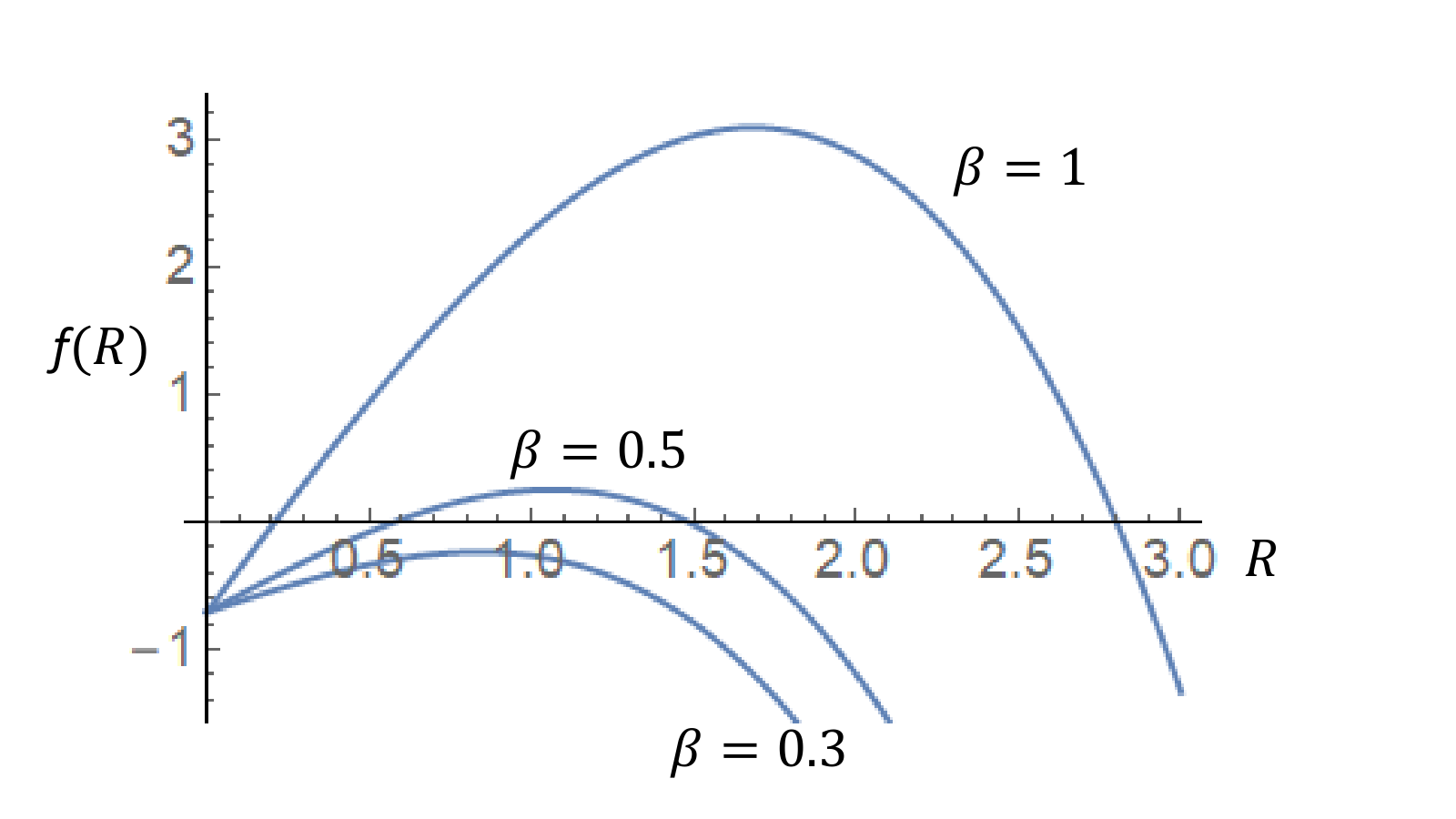
In Fig. 2 we plot the function $f(R)$ for several values of $\beta$ for some values of parameters, these graphs show the existence of two stationary radii, stable and unstable, for $\beta=1$ and $\beta=0.5$ , while no stationary states for $\beta=0.3$ . Therefore, there exists a critical value $\beta_{c}$ such that there are no stationary solutions when $\beta<\beta_{c}$ . Below we find that $\beta_{c}=0.41$ .

Indeed, the critical value $\beta_{c}$ has to satisfy three constraints: (i) $MR_{0}^{2}+\Omega(\beta_{c})-B>0$ , which guarantees the existence of maximum of $f(R)$ at a certain $R=R_{*}$ , (ii) $f(R_{*},\beta_{c})=0$ , (iii) $f^{\prime}_{R}(R_{*},\beta_{c})=0$ . As a result we find that $\beta_{c}$ is the positive solution of the quadratic equation

MR_{0}^{2}+\Omega(\beta_{c})-B=\frac{3}{2}\sqrt[3]{MD_{u}},

(18)

which can be found explicitly. For values of parameters indicated in Fig. 1 we fined $\beta_{c}=0.41$ .

In Fig. 3 we present the numerical solution of the ODE (17) for the values $\beta=1$ and $0.5$ . As we can see, the circular front radius can increase or decrease monotonically until it reaches the steady state value. This is because of the volume is not conserved but influences the dynamics through the parameter $\delta(r,t)$ . For the value $\beta=0.3$ the cell shrinks until it disappears, which means that for such values of parameters, the model does not reflect the true behavior of cells.

IV Dynamics of general cell shape

IV.1 Evolution equation

In this section we consider the evolution of a non-axisymmetric cell shape. We employ the same scaling and definitions as in the previous section. When considering the contributions of derivatives with respect to the azimuthal variable, we use the following expressions:

	$\displaystyle\partial_{\theta}\rightarrow-\epsilon^{-1}R_{\theta}\partial_{z}+\partial_{\theta}$
	$\displaystyle\partial_{\theta}^{2}\rightarrow\epsilon^{-2}R_{\theta}^{2}\partial_{z}^{2}-\epsilon^{-1}(R_{\theta\theta}\partial_{z}+2R_{\theta}\partial_{z\theta}^{2})+\partial_{\theta}^{2}$
	$\displaystyle\frac{1}{r}\partial_{\theta}=-\frac{R_{\theta}}{R}\partial_{z}+O(\epsilon),\ \ \frac{1}{r^{2}}\partial_{\theta}=-\epsilon\frac{R_{\theta}}{R^{2}}\partial_{z}+O(\epsilon^{2})$
	$\displaystyle\nabla^{2}=\left(1+\frac{R_{\theta}^{2}}{R^{2}}\right)u_{zz}+$
	$\displaystyle\frac{\epsilon}{R}\left(u_{z}-\frac{R_{\theta\theta}}{R}u_{z}-\frac{2R_{\theta}}{R}u_{z\theta}-\frac{2zR_{\theta}^{2}}{R^{2}}u_{zz}\right)+O(\epsilon^{2}).$		(19)

We approximate the nonlocality in (3b) as follows,

\int u(x,y,t)\textrm{d}x\textrm{d}y\sim\frac{\epsilon^{-2}}{2}\int_{0}^{2\pi}R^{2}(\theta,t)\textrm{d}\theta.

The same expansions (11) are applied. Define the auxiliary function

\Lambda(\theta,t)=\left(1+\frac{R_{\theta}^{2}}{R^{2}}\right)^{-1/2}

and perform the proper change of variable,

z=\Lambda^{-1}\zeta.

At the leading order we find,

	$\displaystyle D_{u}\Lambda^{-2}u_{0zz}=(1-u_{0})(\frac{1}{2}-u_{0})u_{0},$
	$\displaystyle D_{p}\Lambda^{-2}p_{0zz}-\tau^{-1}p_{0}=\beta u_{0z},$
	$\displaystyle D_{p}\Lambda^{-2}q_{0zz}-\tau^{-1}q_{0}=-\beta\frac{R_{\theta}}{R}u_{0z},$

therefore similarly to the previous section one can calculate the solutions


	$\displaystyle u_{0}(z)=\frac{1}{2}\left[1-\tanh\left(\frac{\zeta(z)}{\sqrt{8D_{u}}}\right)\right],$		(20a)
	$\displaystyle p_{0}(z)=\beta\Lambda\Phi(\zeta)$		(20b)
	$\displaystyle q_{0}(z)=-\beta\Lambda\frac{R_{\theta}}{R}\Phi(\zeta)$		(20c)

The equations for $u$ at the order $O(\epsilon)$ have the form,

	$\displaystyle D_{u}\Lambda^{-2}u_{1zz}-\left(\frac{1}{2}-3u_{0}+3u_{0}^{2}\right)u_{1}=-R_{t}u_{0z}+$
	$\displaystyle D_{u}\left(-\frac{u_{0z}}{R}+\frac{R_{\theta\theta}}{R^{2}}u_{0z}+\frac{2R_{\theta}}{R^{2}}u_{0z\theta}+\frac{2zR_{\theta}^{2}}{R^{3}}u_{0zz}\right)$		(21)
	$\displaystyle+Au_{0z}\left(p_{0}-\frac{R_{\theta}}{R}q_{0}\right)+$
	$\displaystyle(1-u_{0})u_{0}\left\{B+M\left[\frac{1}{2\pi}\int_{0}^{2\pi}R^{2}(\theta,t)\textrm{d}\theta-R_{0}^{2}\right]-S(p_{0}^{2}+q_{0}^{2})\right\}.$

Denote $a=1/\sqrt{2D_{u}}$ . While applying the solvability condition, one has to calculate the following integrals,

	$\displaystyle\int_{-\infty}^{\infty}\textrm{d}zu_{0z}\left(-\frac{u_{0z}}{R}+\frac{R_{\theta\theta}}{R^{2}}u_{0z}+\frac{2R_{\theta}}{R^{2}}u_{0z\theta}+\frac{2zR_{\theta}^{2}}{R^{3}}u_{0zz}\right)=$
	$\displaystyle-a\kappa(\theta,t),\quad\kappa(\theta,t)=\frac{R^{2}+2R_{\theta}^{2}-RR_{\theta\theta}}{(R^{2}+R_{\theta}^{2})^{3/2}},$		(22)
	$\displaystyle\int_{-\infty}^{\infty}\textrm{d}zu_{0z}^{2}\left(\bar{p}-\frac{R_{\theta}}{R}\bar{q}\right)=\beta\Omega_{1},$		(23)
	$\displaystyle\int_{-\infty}^{\infty}\textrm{d}zu_{0z}u_{0}(1-u_{0})(p_{0}^{2}+q_{0}^{2})=\beta^{2}\Omega_{2}.$		(24)

For the first integral (22) we refer the reader to Hamed and Nepomnyashchya 2016 where we calculate the same expression in details. For the integrals (23), (24), notice that the terms dependent on $(\theta,t)$ are vanish. The solvability condition yields a closed evolutionary equation for the front dynamics of the cell, which is an integro-differential equation, i.e., it is nonlocal, unlike that obtained in the circular case (17),

	$\displaystyle a\Lambda R_{t}=-aD_{u}\kappa(\theta,t)$		(25)
	$\displaystyle-\left\{B+M\left[\frac{1}{2\pi}\int_{0}^{2\pi}R^{2}(\theta,t)\textrm{d}\theta-R_{0}^{2}\right]\right\}+\Omega(\beta),$

where $\kappa$ is the mean curvature. Indeed the radial dynamics (16) is recovered, if $R$ does not depend on $\theta$ . By a proper scaling transformation, $t\rightarrow a^{2}t$ and $R(t)\rightarrow aR(t)$ , the equation of motion of the cell boundary can be brought to a canonical form,

v_{n}=-D_{u}\kappa-\delta V+\Omega.

Here we denote

\delta V(t)=B+M\left[\frac{1}{2\pi}\int_{0}^{2\pi}R^{2}(\theta,t)\textrm{d}\theta-R_{0}^{2}\right].

Notice that in (25) the expression $\Lambda R_{t}$ corresponds to the normal velocity of the interface, thus that equation is a generalization of the well-known curvature flow. In addition it suggests an answer for the unrevealed force – velocity relation for the actin network that was highlighted in Keren et al. 2008.

In Fig. 4, the results of the numerical simulation of the fluctuation $\delta R=R(\theta,t)-R_{0}\ll 1$ , which has been carried out using equation (25), are shown. We employ the DSolve function of Mathematica Wolfram. Notice that the fluctuation is relaxed to constant value, that means that any slightly deformed shape will relax to some circular shape, in agreement with the result of the next subsection.

IV.2 Stability of the circular cell shape

For investigating the stability of the circular stationary front $\bar{R}(t)$ that is governed by (17) we substitute the disturbance,

R(\theta,t)=\bar{R}(t)+\hat{R}(\theta,t),

into equation (25). The linearized equation for a small front deformation is

\hat{R}_{t}=D_{u}\frac{\hat{R}+\hat{R}_{\theta\theta}}{\bar{R}^{2}}-\frac{M}{3\pi a}\bar{R}\int_{0}^{2\pi}\hat{R}\textrm{d}\theta,

subject to a boundary condition

R(\theta+2\pi,t)=R(\theta,t).

Let us consider the evolution of a mode

\hat{R}=\varphi_{k}(t)\textrm{e}^{ik\theta},\;k\in\mathbb{Z},

with a definite azimuthal number $k$ . Only for the mode with $k=0$ , which corresponds to a change of the circle radius, the integral term in (25) contributes into the evolution equation for the disturbance. We find that

\partial_{t}\varphi_{0}=\lambda(t)\varphi_{0},

where

\lambda(t)=\sqrt{2D_{u}}\frac{d}{dR}\left(\frac{f(R)}{R}\right)\left|{}_{R=\bar{R}(t)}=\frac{D_{u}}{\bar{R}^{2}(t)}-\frac{2M\bar{R}(t)}{3\pi a}.\right.

For sufficiently small $\bar{R}(t)$ , the disturbance $\varphi_{0}$ can grow, but when $\bar{R}(t)$ approaches its stationary values, the derivative $d(f(R)/R)/dr$ at $R=\bar{R}(t)$ becomes negative (see Fig. 2), hence the circular cell is stable with respect to circular disturbances, as it was shown in the previous section.

For any non-axisymmetric normal modes, $k\neq 0$ , we obtain,

\partial_{t}\varphi_{k}=\frac{D_{u}(1-k^{2})}{\bar{R}^{2}}\varphi_{k}.

The disturbances with $|k|=1$ correspond to a spatial shift of the circle and do not change with time. Disturbances with $|k|\geq 2$ , which describe the shape distortions, decay with time. Thus, a small deformation of the circular shape does not produce any instabilities, in agreement with numerical study of Ziebert et al. 2012. Note that a finite-amplitude disturbance can generally generate an instability.

IV.3 The limit of $R_{\theta}^{2}/R^{2}\ll 1$ and the Burgers-like equation

As the next step, let us consider a nonlinear evolution of a small disturbance satisfying the condition $R_{\theta}^{2}/R^{2}\ll 1$ , hence $\Lambda\sim 1$ .

In that case, the Laplace operator in (19) can be approximated as

\nabla^{2}u=u_{zz}+\frac{\epsilon}{R}\left(u_{z}-\frac{R_{\theta\theta}}{R}u_{z}-\frac{2R_{\theta}}{R}u_{z\theta}\right)+\textit{o}(\epsilon).

(26)

At the leading order we obtain the same solutions $u_{0}(z)$ and $p_{0}(z)$ as in (13) and (14), respectively, and also

q_{0}(z)=-\beta\frac{R_{\theta}}{R}\Phi(z),

While applying the solvability condition to equation (21), we find that

	$\displaystyle\int_{-\infty}^{\infty}u_{0z}^{2}\left(p_{0}-\frac{R_{\theta}}{R}q_{0}\right)\textrm{d}z=\beta\left(1+\frac{R_{\theta}^{2}}{R^{2}}\right)\Omega_{1},$		(27)
	$\displaystyle\int_{-\infty}^{\infty}u_{0}(1-u_{0})u_{0z}(p_{0}^{2}+q_{0}^{2})\textrm{d}z=\beta^{2}\left(1+\frac{R_{\theta}^{2}}{R^{2}}\right)\Omega_{2}.$		(28)

Notice that when calculating (27) and (28) we preserve the negligible expression $R_{\theta}^{2}/R^{2}$ while it is omitted in the approximation of the Laplacian (26).

Finally, the dynamics of the interface is governed by the following nonlinear equation

	$\displaystyle R_{t}=D_{u}\left(\frac{R_{\theta\theta}}{R^{2}}-\frac{1}{R}\right)-$
	$\displaystyle\sqrt{2D_{u}}\delta V(t)+\sqrt{2D_{u}}\Omega(\beta)\left(1+\frac{R_{\theta}^{2}}{R^{2}}\right),$		(29)

with the boundary condition

R(\theta+2\pi,t)=R(\theta,t),

in agreement with Reeves et al. 2018.

Let us consider the fluctuation $\delta R=R(\theta,t)-R_{0}\ll 1$ ; then equation (29) takes the form,

	$\displaystyle\delta R_{t}=D_{u}\left(\frac{\delta R_{\theta\theta}}{R_{0}^{2}}-\frac{1}{R_{0}}+\frac{\delta R}{R_{0}^{2}}\right)-$
	$\displaystyle\sqrt{2D_{u}}\delta V(t)+\sqrt{2D_{u}}\Omega(\beta)\left(1+\frac{\delta R_{\theta}^{2}}{R_{0}^{2}}\right),$		(30)

with the boundary condition

\delta R(\theta+2\pi,t)=\delta R(\theta,t).

Notice that in (30) we preserve leading, first-order correction and quadratic terms.

Applying the operator $\partial_{\theta}$ to the both sides of equation (30) and denoting $G=\partial_{\theta}\delta R$ , we obtain the following nonlinear evolution equation,

\partial_{t}G=\frac{D_{u}}{R_{0}^{2}}\left(\partial_{\theta}^{2}G+G+\sqrt{\frac{2}{D_{u}}}\Omega(\beta)\partial_{\theta}G^{2}\right).

(31)

The solution should satisfy the periodicity condition

G(\theta+2\pi,t)=G(\theta,t),

and the condition

\int_{0}^{2\pi}G(\theta,t)d\theta=0,

which follows from the periodicity of $\delta R$ and definition of $G$ . The obtained equation resembles the Burgers equation, but it contains an additional linear term that can lead to a local growth of $G$ . An equation similar to (31) was studied in Mikishev and Sivashinsky 1993 in another physical context.

The results of the numerical simulation of the temporal evolution of the fluctuation $\delta R$ in the frameworks of equations (30) and (25) almost coincide, see Fig. 4. Therefore, equation (30) may be considered as a reasonable simplification of the more rigorous and general equation (25). Note however in the case when the initial curvature is large in some points the simulation revel a significant deference in the behavior of solutions of (25), (30) see Fig. 5 and 6.

V Conclusion

We have performed an analysis of the cell surface dynamics in the framework of the minimal phase field model of cell motility that was developed and investigated numerically in Ziebert et al. 2012, Ziebert and Aranson 2014, and Ziebert and Aranson 2016, where the order parameter $u$ is coupled with polarization (orientation) vector field P of the actin network. We considered the axisymmetric case (circular shape interface), where we obtained a closed ordinary differential equation describing the evolution of the radius (17). We found the minimum value $\beta_{c}$ for the actin creation that is compatible with the existence of a stationary cell solution (18). We found that when $\beta_{c}<\beta$ , the circular cell can have some stationary radius, while in the case $\beta\leq\beta_{c}$ the cell shrinks until it disappears, which is meaningless in the context of cell dynamics. Also, we consider the general shape cell dynamics. We found the leading order solutions, (20a)-(20c), and derived a closed integro-differential equation (25) governing the cell dynamics, which includes the normal velocity of the membrane, curvature, volume relaxation rate, and a parameter $\Omega$ determined by the molecular effects of the subcell level.

We found an equation of motion of the cell interface that can be written in the canonical form,

v_{n}=-D_{u}\kappa-\delta V+\Omega.

Finally we considered a simplification of our main equation, (25), in the limit $R_{\theta}^{2}/R^{2}\ll 1$ , and obtained a Burgers-like equation (30) for evolution of a small fluctuation $\delta R$ . Fig. 4 confirm such approximation, since the numerical solutions of the both equations (25) and (30) almost coincide. Thus, the result of Reeves et al. 2018, obtained with diffusion terms neglected, is recovered from our more rigorous and precise equation (25). However for other values of parameters and when the initial curvature is large in some points the simulations of equations (25), (30) revel a significant deference see Fig. 5-6.

References

Ziebert et al. (2012) F. Ziebert, S. Swaminathan, and I. S. Aranson, “Model for self-polarization and motility of keratocyte fragments,” J. R. Soc. Interface 9, 1084–1092 (2012).
Kendall (2018) P. Kendall, “How biologists are creating life-like cells from scratch,” nature-news feature 563, 172 (2018).
Kolmakova et al. (2010) G. V. Kolmakova, V. V. Yashina, S. P. Levitan, and A. C. Balazs, “Designing communicating colonies of biomimetic microcapsules,” PNAS 107 (2010).
Kolmakov et al. (2012) G. V. Kolmakov, A. Schaefer, I. Aranson, and A. C. Balazs, “Designing mechano-responsive microcapsules that undergo self-propelled motion,” Soft Matter 8 (2012).
Toohey et al. (2007) K. S. Toohey, N. R. Sottos, J. A. Lewis, J. S. Moore, and S. R. White, “Self-healing materials with microvascular networks,” nature materials-Letters 6, 581 (2007).
Andersson et al. (2007) A. Andersson, J. Danielsson, Astrid Gräslund, and L. Mäler, “Kinetic models for peptide-induced leakage from vesicles and cells,” Eur Biophys J 36, 621–635 (2007).
Mogilner (2008) A. Mogilner, “Mathematics of cell motility: have we got its number?” Mathematical Biology 58, 105–134 (2008).
Ziebert and Aranson (2016) F. Ziebert and I. S. Aranson, “Computational approaches to substrate-based cell motility,” npj Computational Materials 6 (2016).
Nickaeen et al. (2017) M. Nickaeen, I. L. Novak, S. Pulford, A. Rumack, J. Brandon, B. M. Slepchenko, and Alex Mogilner, “A free-boundary model of a motile cell explains turning behavior,” PLOS Computational Biology (2017).
Shao et al. (2010) D. Shao, W. J. Rappel, and H. Levine, “Computational model for cell morphodynamics,” Physical Review Letters 105 (2010).
Camley et al. (2017) B. A. Camley, Y. Zhao, B. Li, H. Levine, and W. J. Rappel1, “Crawling and turning in a minimal reaction-diffusion cell motility model: Coupling cell shape and biochemistry,” Physical Review E 95, 621–635 (2017).
Kimptona et al. (2016) L.S. Kimptona, J.P. Whiteley, S.L. Watersa, and J.M. Oliver, “Approaches to myosin modelling in a two-phase flow model for cell motility,” Physica D 318-319, 34–49 (2016).
Ziebert and Aranson (2014) F. Ziebert and I. S. Aranson, “Modular approach for modeling cell motility,” Eur. Phys. J. Special Topics 223, 1265–1277 (2014).
Reeves et al. (2018) C. Reeves, B. Winkler, F. Ziebert, and I. S. Aranson, “Rotating lamellipodium waves in polarizing cells,” Communications Physics , DOI: 10.1038/s42005–018–0075–7 (2018).
Keren et al. (2008) K. Keren, Z. Pincus, G. M. Allen, E. L. Barnhart, G. Marriott, Alex Mogilner, and J. A. Theriot, “Mechanism of shape determination in motile cells,” nature 453 (2008).
Aranson (2016) I. S. Aranson, Physical Models of Cell Motility (Biological and Medical Physics, Biomedical Engineering, 2016).
Hamed and Nepomnyashchya (2016) M. Abu Hamed and A.A. Nepomnyashchya, “Dynamics of curved fronts in systems with power-law memory,” Physica D 328-329, 1–8 (2016).
Mikishev and Sivashinsky (1993) A. B. Mikishev and G. I. Sivashinsky, “Quasi-equilibrium in upward propagating flames,” Physics Letters A 175, 409–414 (1993).