Lyman-alpha Variability During Solar Flares Over Solar Cycle 24 Using GOES-15/EUVS-E
Abstract
The chromospheric Lyman-alpha line of neutral hydrogen (Ly; 1216Å) is the strongest emission line in the solar spectrum. Fluctuations in Ly are known to drive changes in planetary atmospheres, although few instruments have had the ability to capture rapid Ly enhancements during solar flares. In this paper we describe flare-associated emissions via a statistical study of 477 M- and X-class flares as observed by the EUV Sensor on board the 15th Geostationary Operational Environmental Satellite, which has been monitoring the full-disk solar Ly irradiance on 10 s timescales over the course of Solar Cycle 24. The vast majority (95%) of these flares produced Ly enhancements of 10% or less above background levels, with a maximum increase of 30%. The irradiance in Ly was found to exceed that of the 1-8 Å X-ray irradiance by as much as two orders of magnitude in some cases, although flares that occurred closer to the solar limb were found to exhibit less of a Ly enhancement. This center-to-limb variation was verified through a joint, stereoscopic observation of an X-class flare that appeared near the limb as viewed from Earth, but close to disk center as viewed by the MAVEN spacecraft in orbit around Mars. The frequency distribution of peak Ly was found to have a power-law slope of . We also show that increased Ly flux is closely correlated with induced currents in the ionospheric E-layer through the detection of the solar flare effect as observed by the Kakioka magnetometer.
Astrophysics Research Center, School of Maths and Physics, Queen’s University Belfast, UK BT7 1NN SUPA School of Physics & Astronomy, University of Glasgow, UK G12 8QQ NASA Goddard Space Flight Center, Greenbelt Road, Greenbelt, MD USA, 20771 Space Science Lab., University of California, Berkeley Laboratory for Atmospheric and Space Physics, Boulder, CO.
keypoints
Lyman-alpha irradiance variability during solar flares can be comparable to that due to solar rotation, only on much shorter timescales. The Lyman-alpha irradiance of a flare exhibits significant anisotropy (center-to-limb-variation). Enhanced Lyman-alpha in the flare impulsive phase appears to be capable of inducing currents in the ionospheric E-layer.1 Introduction
The Lyman-alpha (Ly; 1216Å) line of neutral hydrogen, resulting from the 2p–1s transition, is the brightest emission line in the solar spectrum. During quiescent solar conditions, the wings of the line are formed in mid-chromosphere (6,000 K), while the core is formed higher up at the base of the transition region (40,000 K). Due to the high abundance of neutral hydrogen in the solar chromosphere, the Ly line is optically thick with a broad central reversal. During solar flares nonthermal electrons deposit large excess energies in the chromospheric plasma, generating localized heating and ionization at the flare footpoints. This results in enhanced Ly emission although to date there have been very few Ly flare profiles recorded at high spectral resolution. Further Ly flare emission must come from the corona, where according to the well-established scenario the hot, dense flare plasma cools down from X-ray temperatures and eventually drains back to the lower atmosphere as coronal rain. However, given that the electron density and the abundance of neutral hydrogen are considerably higher in the chromosphere than the corona, it is assumed that the bulk of the Ly emission discussed in this paper originates at the flare footpoints (Chamberlin et al. (2018)).
Ly photons drive the molecular dissociation of oxygen (O2) in the Earth’s mesosphere, allowing ozone (O3) to form, while the photoionization of nitric oxide (NO) leads to the formation of the dayside ionospheric D-layer (60–90 km; Chubb et al. (1957); Lean (1985); Woods et al. (1995)). Changes in the Sun’s output at these wavelengths can therefore have significant implications for the dynamics and composition of the terrestrial environment. Several studies have reported on variations in Ly due to solar rotation and over the course of solar cycles (Lean & Skumanich (1983); Lilensten et al. (2008); Woods (2008)). Woods et al. (2000) reported that the mean variability of Ly due to the 27-day solar rotation across Solar Cycles 18–22 was 9%, dropping to 5% at solar minimum and increasing to 11% at solar maximum. Solar Ly variability over the course of a solar cycle varied between a factor of 1.5 and 2.1.
The importance of Ly emission from other stars is also being realized as the search for habitable exoplanets intensifies. However, stellar Ly is almost impossible to detect due to extinction by the interstellar medium, and so indirect reconstruction techniques need to be applied (Linsky et al. (2013), e.g.,). Furthermore, the integration times required to measure stellar EUV emission can be as much as 103 s, which would make the detection of any flare-related variations in Ly very difficult (Christian et al. (2003)).
Solar variability in Ly due to solar flares has not been extensively studied, largely due to instrumental limitations and their duty cycles. Canfield & van Hoosier (1980) were among the first to publish temporal variations in the Ly line profile during two solar flares using the NRL spectrograph as part of the Apollo Telescope Mount onboard Skylab. Brekke et al. (1996) reported a 6% increase in Ly irradiance using Upper Atmosphere Research Satellite/Solar-Stellar Irradiance Comparison Experiment (UARS/SOLSTICE), while Woods et al. (2004) reported a 20% increase in the line core and a factor of two increase in the line wings during the famous 28 October 2003 X28 flare from a serendipitous Solar Radiation and Climate Experiment (SORCE) SOLSTICE (McClintock et al. (2005)) observation. While both SOLSTICE instruments capture disk-integrated emission, their cadence is not sufficient for capturing rapid temporal variations during flares. The Large Yield Radiometer (LYRA; Hochedez et al. (2006); Dominique et al. (2013)) instrument on Project for On-Board Autonomy-2 (PROBA2) also captures full-disk Ly emission but with very high cadence (50 ms). Kretzschmar et al. (2013) reported Ly signatures in 11 flares (C- and M-class) using LYRA, with only a 0.6% increase in emission detected during a detailed study of an M2 flare. The authors comment that this unusually low contrast may be due to the severe detector degradation suffered by the Ly channel, but did not give a detailed explanation. Raulin et al. (2013) also reported a 1% increase in Ly emission during seven solar flares using LYRA, but they also did not detect any appreciable ionospheric disturbances.
As Ly is formed in the chromosphere, its temporal variability during flares should mimic that of the nonthermal electrons responsible for chromospheric heating (i.e. impulsive hard X-ray (HXR) bursts). Kretzschmar et al. (2013) discussed how Ly flare emission from LYRA varied more gradually than expected for an impulsively heated chromospheric feature. A similar discrepancy was reported by Milligan & Chamberlin (2016) for the Extreme-ultraviolet Variability Experiment (EVE; Woods et al. (2012)) Multiple EUV Grazing Spectrograph Photometer (MEGS-P) on the Solar Dynamics Observatory (SDO; Pesnell et al. (2012)). In the case of EVE, this was eventually attributed to a Kalman filter used to smooth the data during processing; this was ultimately replaced with a Fourier transform filter (Don Woodraska; Private Communication, 2017). Milligan & Chamberlin (2016) also showed that the Ly lightcurves from the EUV Sensor (EUVS; Viereck et al. (2007); Evans et al. (2010)) on Geostationary Operational Environmental Satellite (GOES)-15 behaved much more impulsively, as expected, consistent with Lyman continuum (LyC) observations from SDO/EVE MEGS-B and with the temporal behaviour of the Ly emission from the flare presented by Woods et al. (2004). In a statistical study of Ly flares Kretzschmar (2015) derived a scaling relationship between the Ly fluence and soft X-ray (SXR) fluence for around 100 M- and X-class flares, using 1-minute averaged GOES-15/EUVS-E data. He found that Ly was around an order of magnitude stronger than X-rays, with a large degree of scatter that was attributed to either geocoronal absorption or inherent complexities of the Ly line formation.
As well as the space weather implications of changes in Ly emission, Milligan et al. (2014) showed that some 6–8% of the energy deposited in the chromosphere by nonthermal electrons can be radiated away by the Ly line alone (1030 erg; see also Milligan et al. (2012)). This single emission line therefore becomes one of the most important observables for studies of flare energetics. Rubio da Costa et al. (2009) reached a similar conclusion (10% of nonthermal energy) using Ly images from the Transition Region and Coronal Explorer (TRACE; Handy et al. (1999)) (Nusinov & Kazachevskaya (2006), see also). Milligan et al. (2017) also showed that the chromosphere responds dynamically to an impulsive disturbance at its acoustic cutoff frequency, as evidenced by 3-minute oscillations in the Ly time profile from GOES-15/EUVS-E, which appeared in phase with similar periodicities measured in the LyC from SDO/EVE and the 1600Å and 1700Å lightcurves from the Atmospheric Imaging Assembly (AIA; Lemen et al. (2011)) also on SDO. Thus some of a flare’s energy could be dispersed via wave damping (kinetic energy), leading to different radiation signatures.
This paper presents a self-consistent, statistical analysis of almost 500 major solar flares observed in Ly emission. The GOES-15/EUVS-E data have clean time profiles, with high signal-to-noise ratios for major events, making quantitative analysis possible. The time series abundantly confirm the recent discovery of an impulsive-phase signature for Ly, akin to that seen in HXR. This opens a new quantitative channel for modeling of the crucially important flare processes at and near the footpoints of coronal magnetic structures. We primarily present a catalog of Ly energetics, frequency distributions, and center-to-limb variations for future solar-terrestrial studies, and to highlight the availability and importance of an under-utilized dataset. Section 2 describes the data analysis techniques, including accounting for the effects of geocoronal absorption. The findings are presented in Section 3, including a section on ionospheric and geomagetic consequences. The conclusions are presented in Section 4.
2 Data Selection and Reduction
The GOES series of spacecraft have been providing a near-uninterrupted measurement of the solar X-ray irradiance since 1975, beginning with GOES-1, via their X-Ray Sensor (XRS) instruments (Hanser & Sellers (1996)). These data have become the “industry standard” for classifying solar flare magnitudes from the peak of the 1-minute averaged 1–8Å channel. After the launch of GOES-8 in 1994, the reported X-rays fluxes were found to differ from those of the earlier GOES satellites due to more accurate calibration. The National Oceanic and Atmospheric Association (NOAA, who provide the data) decided to scale all XRS data from GOES-8 onwards to match those of earlier missions, in order to preserve the long-term record. To recover the “true” X-ray fluxes, the long-channel data (1–8Å) ought to be divided by 0.7, while the short-channel data (0.5–4Å) needs to be divided by 0.85. This correction has not been applied in this study in order to allow comparisons with previous works, although it is factored in to the GOES software in SSWIDL (SolarSoftWare Interactive Data Language; Freeland & Handy (1998)) when computing the total thermal energy since the temperature response functions are based on the corrected data (Kim Tolbert; Private Communication 2019; https://hesperia.gsfc.nasa.gov/rhessidatacenter/complementary_data/goes.html). Only XRS data from GOES-15, with a cadence of 2 s, have been used in this study.
The launch of GOES-13 in 2006 (and subsequently, GOES-14 and -15) saw the inclusion of the EUVS in order to characterize the solar EUV irradiance with a cadence of 10.24 s. EUVS comprises five channels: A, B, C, D, and E, covering the 50–170Å, 240–340Å, 200–620Å, 200–800Å, and 1180–1250Å wavelength ranges, respectively (Viereck et al. (2007)), with the E-channel centered on the Ly line at 1216Å. The E-channel data have been converted to irradiance by scaling to a Whole Heliosphere Interval quiet-Sun reference spectrum (http://lasp.colorado.edu/lisird/data/whi_ref_spectra; Woods et al. (2009)). The conversion to physical units for irradiance will therefore not reflect flare-related time variations of the line profile, generating some systematic uncertainties. Over time, the EUVS-E suffers from degradation, which is compensated for by scaling the daily average values to those from SORCE/SOLSTICE. While Ly measurements from GOES-13 and -14 have been sporadic, GOES-15 has provided continuous coverage since its launch in 2010. GOES-15 continues to take measurements in the EUV although at the time of writing, only data up to 6 June 2016 have been made publicly available (https://www.ngdc.noaa.gov/stp/satellite/goes/doc/GOES_NOP_EUV_readme.pdf). Only Version 4 of the 10.24 s cadence EUVS-E data from GOES-15 were used in this study.
The SDO/EVE instrument has a MEGS-B component, which returns whole-Sun spectra at EUV wavelengths (330-1050Å; Crotser et al. (2007)) with 10 s time resolution and 1Å spectral resolution. The same instrument measures spatially- and spectrally-integrated Ly emission via its MEGS-P photometer, also at 10 s cadence. Unforeseen detector degradation post-launch meant that MEGS-B and -P were only able to observe the Sun in Ly for 3 hours per day, plus 5 minutes every hour for most of the SDO mission, and so it has observed significantly fewer flares than GOES-15 (see Table 1). In 2015, the flight software was updated to have MEGS-P (and MEGS-B) respond to increases in SXR emission detected by its ESP channel, making EVE a dedicated flare instrument. Recently (19 April 2018), to further preserve the signal-to-noise ratio as the instrument deteriorates, the cadence was reduced to 60 s.
| Database | M-class | X-class | Total |
|---|---|---|---|
| NOAA/GOES | 677 | 45 | 722 |
| SSW Latest Events | 573 | 33 | 606 |
| This study | 446 | 31 | 477 |
| SDO/EVE MEGS-P | 94 | 8 | 102 |

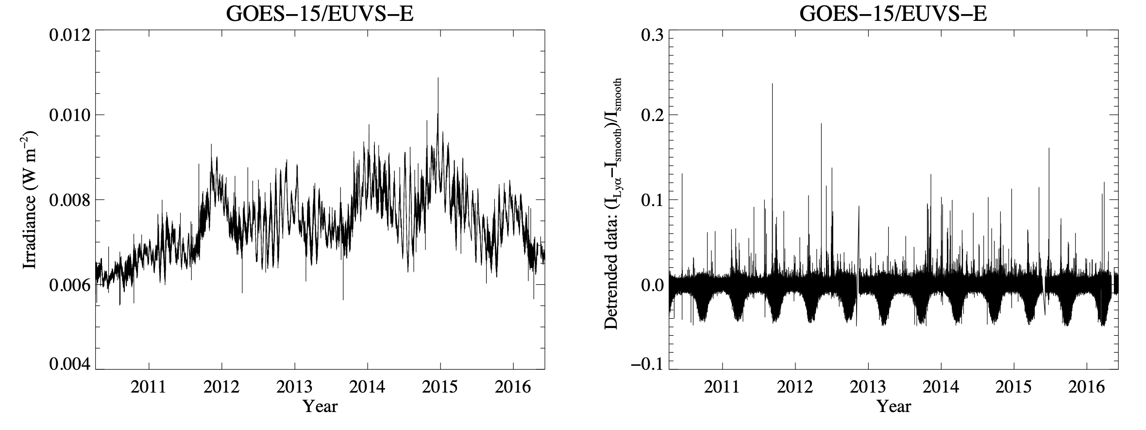
The left-hand panel of Figure 1 shows the complete six years of currently available GOES-15/EUVS-E data covering Solar Cycle 24. The presence of the 27-day period due to active region rotation is clearly visible. By detrending these data (using a 120-point/20 minute smoothing function) to remove solar-cycle and rotation timescales, the biannual eclipse seasons - seen as dips in the time profile in the right-hand panel of Figure 1 - become apparent. These result from geocoronal absorption by the Earth’s uppermost atmosphere, which has substantial opacity to Ly line-core photons (Meier & Prinz (1970); Baliukin et al. (2019)). Note that the timing and depth of this dip varies over the course of the year as the EUVS instrument peers through different column depths of the geocorona throughout its orbit. The daily dips typically last for around 4 hours of local midnight, and range from 0.3–6%, with the greatest decreases occurring at the time of the equinoxes. The geocorona is transparent to X-rays, but there are periods when the GOES satellites are in eclipse, blocking out both X-rays and Ly.
One of the best-established solar flare catalogs available is that from the GOES/XRS photometers, as characterized by the flux of its 1–8Å passband (https://www.ngdc.noaa.gov/stp/solar/solarflares.html). This list is compiled by NOAA and extends back to 1977. Over the six years of available GOES-15/EUVS-E data, the catalog lists the start, peak, and end times of 677 M-class flares and 45 X-class (see Table 1). While the NOAA event list does not always provide heliographic locations for each of these flares, Milligan & Ireland (2018) recently compiled a list of flares observed by multiple instruments during Solar Cycle 24, which included flare locations based on SDO/AIA 94Å (10 MK) difference images. These (coronal) locations were extracted from the SSW Latest Events list, which is accessible through the Heliophysics Events Knowledgebase (HEK; https://www.lmsal.com/hek/). In this study the locations were needed to derive the center-to-limb variation (CLV) of (excess) Ly emission (Section 3.3). However, this database is incomplete and is missing several months of information. Location information was available for 573 M-class and 33 X-class flare in total. Given that the effect of geocoronal absorption on the flare excess emission was assumed to be nonlinear, and therefore difficult to correct for, all events for which the GOES start and/or end time lay within 2 of the minima of all geocoronal dips were omitted. This left a sample of 446 M-class flares and 31 X’s (477 in total). For comparison, from the launch of SDO until 6 June 2016, EVE MEGS-P observed 94 M-class flares and eight X-classes flare in their entirety (between GOES start and end times), not counting those that were partially observing during its 5-minute observing periods.
Figure 2 shows a sample of ten X-class flares in both X-rays (grey curves) and Ly (black curves) to illustrate the quality of the EUVS-E data and to show the variety of Ly responses during flares of comparable X-ray magnitudes. Their GOES classifications and heliographic locations are annotated in the top right corner of each panel. Panel shows the first X-class flare of Solar Cycle 24 as previously reported by Milligan et al. (2012); Milligan et al. (2014), Milligan & Chamberlin (2016), and Milligan et al. (2017). Interestingly, the flare in panel is the largest in the sample (X6.9), but only shows a modest Ly increase, while the more common X1.8 flare in panel exhibited the largest Ly contrast (29% increase) of all the flares studied. Some events displayed multiple Ly bursts (panels , , and ), while others showed no variation due to being either behind (panel ) or close to (panel ) the solar limb. Even back-to-back events of similar magnitudes from the same active region can exhibit substantially different Ly profiles (panel ).
2.1 Background Subtraction
Figure 3 illustrates how background subtracted X-ray and Ly profiles were generated for all flares considered. The top left panel shows XRS data over a 24-hour period centered on the peak of the X2.7 flare that occurred on 5 May 2015 (SOL2015-05-05). For each flare, the background of the 1–8Å channel was taken to be the minimum value within this 24-hour period (denoted by the horizontal red line). The resulting background subtracted profile, between the start and end times of the GOES event (shown as vertical dotted lines in the two left hand panels), is then shown in the top right hand panel. Note that because the largest flares often have peak fluxes several orders of magnitude above the background level, they are not particularly sensitive to background subtraction (Ryan et al. (2012)).
The bottom left-hand panel of Figure 3 shows the corresponding EUVS-E Ly lightcurve over the same 24-hour period. Comparing with the panel above, it is clear that only the largest flares produce enhanced Ly emission above the background level. Also visible is the daily geocoronal absorption dip beginning around 07:00 UT (vertical dashed line). The presence of these geocoronal dips coupled with the fact that changes in Ly due to flares are not as substantial as those in X-rays requires a more careful subtraction of the solar background. The entire 24 hour period was fit with an inverted Gaussian to account for the geocoronal dip, plus a constant equal to the modal value over the time interval. Subtracting this background reveals the flare excess emission between the start and end times of the corresponding GOES event (bottom right hand panel). The ratio of the peak Ly flux relative to the background value then defines the contrast (percentage increase above background; see Section 3.1).

2.2 Flare Energetics
Having established the flare excess emission in both Ly and X-rays between the start and end of each GOES event, the total energy emitted over each wavelength range can be determined by integrating each profile over time. We convert from W m-2 to erg s-1; 1 W m-2 = 2 (1 AU)107 erg s-1=1.4061030 erg s-1. Deviations from 1 AU as the Earth - and therefore, GOES-15 - completes its orbit around the Sun were also accounted for. The flux ratio from the two XRS channels also allows the derivation of a temperature () and emission measure () of the X-ray emitting plasma via the procedure outlined in Garcia (1994) and White et al. (2005). Combining these results with the radiative loss function allows the radiative loss rate by the total SXR emitting plasma to be calculated through the simple expression , where EM = , is the electon density, is the volume, and is the Boltzmann constant (see Section 3.2). Coronal abundances and =1010 cm-3 are assumed by default.
The biggest uncertainty in the determination of the total energy radiated by each mechanism is that of the end time of the flare as specified in the GOES event list. NOAA stipulate this time to be that when the X-ray flux equals half that of the peak value (https://www.ngdc.noaa.gov/stp/solar/solarflares.html). In the largest events, X-rays can remain elevated above the background levels for several hours beyond the cataloged end time, while the impulsive nature of Ly often sees it approach background levels much more rapidly. Accounting for the ‘real’ flare end time would require fitting the decaying emission with an uncertain approximation, say an exponential function, and extrapolating in time. This is beyond the scope of this paper (see also Ryan et al. (2016)). Therefore, to assess the effect of a longer flare duration on the relative energy radiated, the end time of the X-class flare shown in Figure 3 was arbitrarily extended by 90 minutes. As shown in the left hand panel of Figure 4, the X-ray flux (dashed curve) continued to decay beyond the listed end time (vertical solid line), while the Ly flux (solid curve) had almost returned to pre-flare levels. The cumulative radiated energy by the two processes are shown in the right hand panel as cyan curves, along with the background-subtracted lightcurves (black curves). The ratio of the two energies is plotted as a solid red curve, and does not appear to change appreciably between the listed GOES end time and 90 minutes later. The energies for both X-rays and Ly reported in Section 3 can therefore be considered lower limits, although the ratio of the two may be broadly considered independent of the total integration time.
3 Results
3.1 Flare Contrast
Solar flares are known to vary by over two orders of magnitude in the X-ray portion of the spectrum relative to the background emission during the most extreme events (Ryan et al. (2012)), while the corresponding increase in Ly irradiance can be marginal due to the much higher background at this wavelength. The left hand panel of Figure 5 shows a histogram of the peak Ly flux for all flares in this study relative to their pre-flare background. This shows that 95% of flares exhibit a 10% enhancement in Ly, with a maximum contrast of 30%. These variations are comparable to or greater than changes brought about during active region evolution, albeit on much shorter time scales (Woods et al. (2000)). The right hand panel shows how this peak Ly flux varies with the equivalent peak X-ray flux (essentially, GOES class). For M-class flares (10-5 W m-2), peak Ly flux is on average a factor of 10 more intense that that of the X-rays, and as much as a factor of 100 for some events. For X-class flares, the Ly flux averages about three times that of X-ray flux, with a maximum of a factor of 10. This is in agreement with Kretzschmar (2015) who found a similar scaling relationship between Ly and X-ray fluence for around 100 events.
Previous reports of Ly enhancements during flares have often focused on individual or small numbers of events. Woods et al. (2004) reported a 20% increase during an X28 flare observed by SORCE/SOLSTICE, while Milligan et al. (2014) reported an 8% increase during an X2.2 flare observed by SDO/EVE. Kretzschmar et al. (2013) and Raulin et al. (2013) both reported enhancements of 1% using data from PROBA2/LYRA. While the M2 flare presented by Kretzschmar et al. (2013) was not included in this current study, it was observed by GOES-14/EUVS-E which measured a 3% increase, suggesting that LYRA may have been underestimating flare-related enhancements to the solar irradiance. This study now presents a comprehensive overview of the variability of solar Ly irradiance due to major solar flares through a systematic analysis of almost 500 events.
3.2 Flare Energetics
Both Ly and SXR are known drivers of changes in the ionosphere. Therefore knowing the proportional amounts of energy that are injected into the terrestrial atmosphere during flares is important for assessing their relative effects. Milligan et al. (2012) showed that twice as much energy was radiated by Ly compared to X-rays during a single X-class flare that occurred close to disk center, while Kretzschmar (2015) found that the Ly fluence is around an order of magnitude higher than that of SXR for around 100 flares. The left hand panel of Figure 6 shows the total Ly energy radiated relative to the total X-ray energy between the GOES start and end times of each event. Similar to that found for the peak fluxes presented in Section 3.1, and in agreement with Kretzschmar (2015), approximately 1–100 times more energy was radiated via the Ly line than the 1–8Å channel for most M-class flares. X-class flares were only up to 10 times more intense in Ly than in X-rays. Some events showed very weak Ly energies (1028 erg) as they might not have exhibited an appreciable enhancement above the background due to their proximity to the solar limb, either because of opacity effects along the line of sight, or the footpoints or ribbons being foreshortened or occulted by the solar disk (see Section 3.3). Kretzschmar (2015) attributed the weaker events in his correlation to possible geocoronal absorption, which is not the case as those events affected were removed from this analysis.
The right-hand panel of Figure 6 shows the same Ly energies relative to the total thermal energy radiated from the flaring coronal loops as calculated in Section 2.2. In this case, the Ly energies are comparable to, or around a factor of 10 less, than the total thermal energy. The most reliable measurement to date of a flare’s ‘true’ energy stems from observations of flares in the Total Solar Irradiance (TSI) by Woods et al. (2006) using SORCE/Total Irradiance Monitor (TIM; Kopp & Lawrence (2005)). The authors state that the total flare energy is approximately 105 times that of the 1–8Å energy, although this was only measured for four events. Emslie et al. (2012) have summarized these results, finding that the total instantaneous thermal energy accounted for about one fifth of the detected bolometric energy. The findings presented here imply that Ly is indeed a significant radiator of flare energy, as suggested by Milligan et al. (2014).
3.3 Center-to-Limb Variation
As Ly is known to be optically thick (Woods et al. (1995), e.g.,), some degree of center-to-limb variation (CLV) is to be expected, given that Ly emission from flare ribbons nearer the solar limb will be scattered by the chromospheric column mass along the line of sight. Curdt et al. (2008) showed that this was the case for quiescent Ly using spatially-resolved data from SOHO/Solar UV Measurements of Emitted Radiation (SUMER; Wilhelm et al. (1995)). Similarly, Woods et al. (2006) showed that a CLV was also applicable to the handful of flares observed in the TSI by SORCE/TIM. By measuring the total energy in the TSI flare excess relative to that of the GOES X-rays (which are optically thin, and therefore not attenuated by the solar atmosphere), for each event, the ratio, R, as a function of heliocentric angle was fit with the ad hoc quadratic expression
| (1) |
where is the TSI/X-ray ratio at disk center, is the limb variation relative to the center, and =cos() (see Brekke & Kjeldseth-Moe (1994) for the original empirical derivation). Woods et al. (2006) found . The same technique was applied here to Ly flares to allow a comparison with previous works. The left-hand panel of Figure 7 shows as a function of heliocentric angle for X-class flares only, with fits to the data using Equation 1 overplotted. The resulting values of and were 4.33 and 0.12, respectively, in excellent agreement with Woods et al. (2006). The right hand panel of Figure 7 shows the corresponding peak contrast values of Ly for all flares also as a function of heliocentric angles (grey diamonds) with the mean values overplotted as black solid circles with 1 error bars for each integer value of angle. A similar ‘tailing-off’ can be seen towards the limb.


This result can be confirmed with direct, stereoscopic observations of an X-class limb flare (SOL2014-10-19, S13E57, X1.1; denoted by the filled datapoint in the left hand panel of Figure 7). This was was fortuitously observed in Ly by both GOES-15/EUVS-E and the Mars Atmospheric and Volatile Evolution (MAVEN) Extreme Ultraviolet Monitor (MAVEN/EUM; Eparvier et al. (2015)), while Earth and Mars were 88.2∘ apart (see top left panel of Figure 8). MAVEN/EUM also includes a Ly photometer that observes full-disk solar irradiance at 1 s cadence to investigate the impact of solar radiation on the Martian atmosphere. (See Chamberlin et al. (2018) for an overview of flaring activity during the September 2017 period, including Ly observations from MAVEN.) From MAVEN’s vantage point, this flare (top right panel of Figure 8) would have appeared close to disk center (S11W31 at Mars). The corresponding lightcurves from both instruments (at 1 AU, after correcting for the Earth-Mars distance and light travel time) are plotted in the bottom panel of Figure 8. The 45% increase of flare excess emission observed at Mars relative to that seen at Earth, (/) intensity is in good agreement with that predicted by our limb-darkening function (Equation 1). Assuming that the X-ray flux at both vantage points would have been the same, the Ly energy at 30∘ would have been 4.5 times higher than that of the X-rays, while at 60∘ it would have been 3 times higher. This yields a predicted increase of 66% compared to our measured value of 45%. Some discrepancy from calibration uncertainties would be expected, or from a more complete form of limb darkening, which might depend upon source geometry as well as limb distance.
3.4 Frequency Distributions
An important property of solar flares (along with other systems exhibiting self-organized criticality) is the slope of the frequency distribution of event occurrence. It has been well established for decades that flare distributions can be well represented with a power law of the form:
| (2) |
where is the frequency distribution of a flare parameter, , is the power-law index, and is a scaling constant. In the case of coronal (e.g. EUV) emission, a value of would imply that, extending the distribution to lower energies, would contain enough energy to heat the solar corona (Hudson (1991)). This analysis has since been carried out over a wide range of wavelengths (HXR; Hannah et al. (2011), EUV brightenings; Parnell & Jupp (2000), SXR; Veronig et al. (2002)). Traditionally, the approach has been to bin the data (e.g. peak flux) logarithmically and fit the distribution with a power-law function. Kretzschmar (2015) applied this technique to a sample of 100 Ly flares and derived a value of between 2.3 and 2.9. However, this method is prone to selection effects, based on the bin sizes (Bai (1993); Ryan et al. (2016), e.g.). Using a Maximum Likelihood method instead removes most of these issues. We adopted the double power-law approach of Parnell & Jupp (2000), which not only determines the power-law index, , but also the break in the double power-law, above which the well-sampled distribution can be reliably determined. This flattening of the distribution at lower fluxes is a well known selection effect in which the weaker events are harder to detect and hence undersampled (Hannah et al. (2011); Aschwanden (2011)).
The resulting empirical frequency distribution and power-law fit for our peak Ly flux is shown in Figure 9. Here an index of was found for fluxes above W m-2. This index lies close to the upper end of the range found by Kretzschmar (2015) and is steeper than those found for the X-ray and other flare observables ( for HXR bursts; Dennis (1985), for SXR fluxes; Veronig et al. (2002)). Where the empirical frequency distribution matches the power-law line in Figure 9 there is a good fit to the data. At higher fluxes we see that there are significantly fewer events than predicted by power law we have found, hinting at a physical effect limiting the event numbers. A similar roll-over has been seen in other flare frequency distribution - for instance, in HXR flare observations from Ulysses (Tranquille et al. (2009)) - but given the infrequency of the largest events, other approaches are often required to better constrain the power law nature of the largest events (Schrijver et al. (2012)).
3.5 Ionospheric and Geomagnetic Consequences

Ionization resulting from solar UV and X-ray emission dominates the Earth’s dayside ionosphere. Solar flares provide sudden changes in this ionizing radiation, and Ly carries a substantial fraction of the flare perturbations. While disturbances can occur in all regions of the ionosphere following a flare, the effects on the lowest lying regions, typically the D- and E-regions, are most apparent. SXR flare emission is thought to play the largest role as it can vary by several orders of magnitude during major events, but can also penetrate down to low ionospheric altitudes to significantly increase electron density in the D-region. This response can be probed through the observation of Very Low Frequency (VLF 3-30kHz) radio signal amplitude and phase. Ly should also have a significant effect in these ionospheric regions, although there has been no comprehensive and systematic monitoring of Ly at high time cadence as are now available from GOES. This will help to characterize the ionospheric response to enhanced Ly flaring emission.
The major impulsive flare SOL2011-09-07 was chosen to identify the possible effect of flare-related changes in Ly on the ionosphere through observations of enhanced conductivity recorded at the Kakioka magnetometer, Japan and VLF amplitude measurements at a Stanford Sudden Ionospheric Disturbance receiver located in River Heights, Utah. The receiver measures the 24kHz VLF amplitude from the NAA transmitter located in Cutler, Maine (top panel of Figure 10). The time-series of these observations together with the GOES Ly and 1-8Å emission are shown in the bottom panel. This figure shows that the absolute flux increase in Ly (black curve) is approximately an order of magnitude greater than that of the SXR (blue curve). The response of the ionosphere can also be clearly identified both in the magnetometer data (E-layer; green) and the VLF data (D-layer; blue). Notably, the inset plot clearly illustrates that the timing of the (normalized) geomagnetic disturbance, known as the “Solar Flare Effect” (Sfe), closely matches the Ly profile, while the SXR emission peaks several minutes later, followed by the VLF amplitude. This indicates that it is not the SXR emission driving the geomagnetic disturbance as observed in the magnetometer data, but the impulsive Ly emission.
It is particularly interesting that an impulsive Sfe in the magnetometer (westward) Y-component was observed to closely match the impulsive time scale of Ly, rather than the SXR. This hints at enhanced E-region (90–150 km) current systems perpendicular to the magnetic field due to the ionization of NO by the large energy flux of the Ly line, as opposed to ionization in the D-layer which is less electrically conductive due to electron-neutral collisions. This goes against the currently accepted theory that (non-flaring) solar SXR are responsible for ionizing NO (Barth et al. (1988); Barth et al. (1999); Siskind et al. (1990); Siskind et al. (1995); Bailey et al. (2002); Fuller-Rowell et al. (2004), and references therein) at these altitudes. We also note that this event produced the largest Ly enhancement of all the flares in our study and so may have been a unique case; perhaps NO abundances in the E-layer were significantly higher at the time of this event. There may also have been seasonal or solar cycle effects to consider. A geomagnetic Sfe in fact appeared in conjunction with the first-ever recorded solar flare, SOL1859-09-01 (Carrington (1859); Stewart (1861)) in the form of deflections seen in a “self-recording magnetograph.”
The D-region response to solar flares, as measured by VLF amplitude observations, often closely matches the SXR flare emission and typically do not show a good correlation with the more impulsive Ly (Raulin et al. (2013), e.g.). During quiet solar conditions the unperturbed daytime D-region is maintained by Ly emission acting on minor constituent NO, however during a flaring event the increased SXR penetrates down to D-region altitudes to dominate ionization of neutral constituents including N2 and O2. This markedly increases electron density in this region large enough to change the propagation conditions of VLF radio waves, and hence the flare response is reflected in the VLF amplitude measurements (Thomson & Clilverd (2001); Thomson et al. (2005)). The 3-minute time-delay between the SXR and VLF amplitude, shown in Figure 10, is characteristic of the D-region, known as the ‘sluggishness’ of the ionosphere (Appleton (1953)) and signifies the time taken for the D-region photoionization-recombination processes to recover balance after increased ionization (Žigman et al. (2007), see also). This case study however clearly shows that flare Ly can have an impact on the ionospheric response (potentially at higher altitudes) in addition to the SXR flux which is typically thought to be the main driver of flare-driven ionization. The availability of high-cadence Ly data from GOES-15 (and from future GOES missions) allows for the systematic investigation of the relative timings of the Sfe.
4 Conclusions
This paper presents an overview of over six years of solar flare observations in Ly emission (477 events) taken with the E-channel of the EUVS instrument on GOES-15. Prior to this, Ly flare observations had been severely limited, with sometimes contradictory results, hampering the understanding of how these events contribute to the broader field of space weather. After removing flaring events that were affected by geocoronal absorption, this work shows that Ly is significantly (1–100) more energetic than the more commonly studied SXR (1–8Å), which are also a driver of ionospheric disturbances, in agreement with an earlier study of 100 events by Kretzschmar (2015). We also show that Ly enhancements are comparable to those due to solar rotation, though on timescales of minutes rather than months. However, the Ly contribution is less significant for flares that occur close to the solar limb, due to either opacity effects, or foreshortening or occultation of the flare footpoints as seen from Earth. This center-to-limb variation was verified through a simultaneous observations of a limb flare that was also observed by MAVEN/EUM when Earth and Mars were 90 degrees apart. The frequency distribution of peak Ly flux revealed a power law slope of =2.8, implying that the cumulative input from smaller flares may pose a greater energetic input into Earth’s atmosphere than the summation of larger events.
The high time cadence of the GOES-15/EUVS-E data also allows a more comprehensive comparison of the relative ionospheric effects between Ly and X-rays. Using magnetometer data from Kakioka it was found that increased conductivity in the ionosphere in response to a major solar flare was highly correlated with with the increase in Ly flux, while the corresponding increase in X-rays lagged by several minutes, indicating that the X-rays could not have been the driver of the initial geomagnetic impulse. Our observations suggests that the Ly driven Sfe occurs in the E-region, rather than the D-region, and may explain why no such ionospheric response (as characterized by a VLF phase change) was identified by Raulin et al. (2013) during seven solar flares observed by PROBA2/LYRA. The flares that they studied were also of a lower magnitude that those presented here (C- and low M-class), and were therefore unlikely to have produced any enhancement above the solar Ly background. Some of these flares also occurred close to the solar limb further diminishing the possibility of them contributing to variations in the solar Ly irradiance.
While the most recent GOES-15 Ly data (including those from the period of intense flaring activity in September 2017) have not yet been released at the time of writing, the heliophysics and space weather communities are also anticipating further Ly observations from the next generation of GOES satellites, the GOES-R series. These four spacecraft include a dedicated suite of EUV (Eparvier et al. (2009)) and X-ray (Chamberlin et al. (2009)) instruments (EUV and X-ray Irradiance Sensors; EXIS), which will provide more advanced coverage of the Sun’s output over the next 20 years or more. The Ly line will be sampled across five spectral bins, giving a rough estimate of variations in the full-disk line profile.
Ly also plays a very important role in trying to understand the physical processes that underpin solar flares themselves. The current study confirms that flare Ly emission has a clear impulsive-phase peak. It had been established that Ly is a significant radiator of flare energy, but this behavior also means that the data can be used to provide clues as to how the solar chromosphere and transition region respond to flare energy release. Future flare studies could look at the link between Ly and LyC (Machado et al. (2018)), or Ly and H (Canfield et al. (1981)), for example. The recent launch of Solar Orbiter also included an Extreme Ultraviolet Imager (EUI; Schühle et al. (2011); Rochus et al. (2020)) that contains a Ly channel as part of its High Resolution Imager (HRI) suite. EUI will image the Sun in Ly at 1 s cadence, at 1′′ resolution at 0.3AU. The currently proposed Japanese Solar-C mission (the follow up to Hinode) is also expected to feature a Ly spectrograph (Teriaca et al. (2011)), as well as the Lyman-alpha Solar Telescope (LST) on the Chinese ASO-S satellite (Li (2016)). The findings presented here will also assist in the interpretation of results from these future observing platforms.
Acknowledgements.
ROM would like to thank Kim Tolbert at NASA/GSFC for her help with making the GOES/EUVS data easily accessible, Janet Machol at NOAA for her advice and assistance, Hamish Reid for several stimulating discussions, and to Edward Cliver for bringing the Kakioka data to our attention; we thank the Kakioka Magnetic Observatory for providing these data (http://www.kakioka-jma.go.jp/obsdata/metadata/en). ROM would also like to thank Science and Technologies Facilities Council (UK) for the award of an Ernest Rutherford Fellowship (ST/N004981/1), and to the University of Glasgow for a Lord Kelvin Adam Smith award. PCC would like to acknowledge funding from NASA Living with a Star Grant NNX16AE86G titled “Improving Solar EUV Spectral Irradiance Models with Multi-Vantage Point Observations”. IGH is supported by a Royal Society University Fellowship. LAH is supported by an appointment to the NASA Postdoctoral Program at Goddard Space Flight Center, administered by USRA through a contract with NASA. The GOES and MAVEN data used in this study are freely and publicly available from the instrument websites (GOES/EUVS: https://satdat.ngdc.noaa.gov/sem/goes/data/euvs/GOES_v4/G15/; GOES/XRS: https://www.ngdc.noaa.gov/stp/satellite/goes/dataaccess.html; MAVEN/EUM: https://lasp.colorado.edu/lisird/data/mvn_euv_l2_bands/). The VLF data is available from the Stanford Sudden Ionospheric Disturbance database (http://sid.stanford.edu/database-browser/). All the authors would like to thank the four anonymous referees for their helpful comments, and editor Mike Hapgood in particular for his support and encouragement.Appendix A Acoustic Oscillations in MAVEN/EUM data
As mentioned in Section 1, Milligan et al. (2017) detected 3-minute oscillations in full-disk Ly emission from GOES-15 during the 15 February 2011 (SOL2011-02-15) X-class flare. This was interpreted as the generation or enhancement of acoustic waves in the chromosphere in response to the impulsive release of energy during the initial stages of the flare. The oscillation was found to be independent of rate of heating due to nonthermal electrons as determined from HXR observations. To date, this is the only reported case of acoustic oscillations in full-disk EUV irradiance data. However, for the X-class flare described in Section 3.3 (SOL2014-10-19), the standard wavelet analysis of Torrence & Compo (1998) was applied to the Ly lightcurve from MAVEN/EUM. Figure 11 shows that the wavelet power around the onset of the flare is also enhanced at a period of 4.4 minutes, indicative of flare-induced acoustic waves. This deviates slightly from the value found by Milligan et al. (2017) but Jess et al. (2013) shows that the inclination of the magnetic field can affect the periodicity of propagating disturbances in the chromosphere.

References
- Appleton ((1953)) Appleton, E.V. (1953). A note on the ÒsluggishnessÓ of the ionosphere. Journal of Atmospheric and Terrestrial Physics 3 5 282–284.
- Aschwanden ((2011)) Aschwanden, M.J. (2011). The State of Self-organized Criticality of the Sun During the Last Three Solar Cycles. I. Observations. Sol. Phys. 274 1-2 99-117. doi:10.1007/s11207-011-9755-0
- Bai ((1993)) Bai, T. (1993). Variability of the occurrence frequency of solar flares as a function of peak hard X-ray rate. ApJ 404 805-809. doi:10.1086/172335
- Bailey et al. ((2002)) Bailey, S.M., Barth, C.A. & Solomon, S.C. (2002). A model of nitric oxide in the lower thermosphere. Journal of Geophysical Research (Space Physics) 107 A8 1205. doi:10.1029/2001JA000258
- Baliukin et al. ((2019)) Baliukin, I.I., Bertaux, J.L., Quémerais, E., Izmodenov, V.V. & Schmidt, W. (2019). SWAN/SOHO Lyman- Mapping: The Hydrogen Geocorona Extends Well Beyond the Moon. Journal of Geophysical Research: Space Physics 124 2 861–885.
- Barth et al. ((1999)) Barth, C.A., Bailey, S.M. & Solomon, S.C. (1999). Solar-terrestrial coupling: Solar soft X-rays and thermospheric nitric oxide. Geophys. Res. Lett. 26 9 1251-1254. doi:10.1029/1999GL900237
- Barth et al. ((1988)) Barth, C.A., Tobiska, W.K., Siskind, D.E. & Cleary, D.D. (1988). Solar-terrestrial coupling: Low-latitude thermospheric nitric oxide. Geophys. Res. Lett. 15 1 92-94. doi:10.1029/GL015i001p00092
- Brekke & Kjeldseth-Moe ((1994)) Brekke, P. & Kjeldseth-Moe, O. (1994). The solar UV continuum 1440–1680 Å and its center-to-limb variation. Solar Physics 150 1-2 19–47.
- Brekke et al. ((1996)) Brekke, P., Rottman, G.J., Fontenla, J. & Judge, P.G. (1996). The Ultraviolet Spectrum of a 3B Class Flare Observed with SOLSTICE. ApJ 468 418. doi:10.1086/177701
- Canfield et al. ((1981)) Canfield, R.C., Puetter, R.C. & Ricchiazzi, P.J. (1981). The Lyman-alpha/H-alpha ratio in solar flares and quasars. Astrophysical Journal 249 383–389.
- Canfield & van Hoosier ((1980)) Canfield, R.C. & van Hoosier, M.E. (1980). Observed L-alpha profiles for two solar flares - 14:12 UT 15 June, 1973 and 23:16 UT 21 January, 1974. Sol. Phys. 67 339-350. doi:10.1007/BF00149811
- Carrington ((1859)) Carrington, R.C. (1859). Description of a Singular Appearance seen in the Sun on September 1, 1859 . Mon. Not. R. Astr. Soc. 20 13-16.
- Chamberlin et al. ((2018)) Chamberlin, P.C., Woods, T.N., Didkovsky, L., Eparvier, F.G., Jones, A.R., Machol, J.L.Woodraska, D.L. (2018). Solar Ultraviolet Irradiance Observations of the Solar Flares During the Intense September 2017 Storm Period. Space Weather 291 6 1665.
- Chamberlin et al. ((2009)) Chamberlin, P.C., Woods, T.N., Eparvier, F.G. & Jones, A.R. (2009). Next generation x-ray sensor (XRS) for the NOAA GOES-R satellite series. In Solar physics and space weather instrumentation iii. edited by fineschi, silvano; fennelly, judy a. proceedings of the spie, volume 7438, article id. 743802, 10 pp. (2009). ( 7438, p. 743802). doi:10.1117/12.826807
- Christian et al. ((2003)) Christian, D.J., Mathioudakis, M., Jevremović, D., Dupuis, J., Vennes, S. & Kawka, A. (2003). The Extreme-Ultraviolet Continuum of a Strong Stellar Flare. ApJ 593 2 L105-L108. doi:10.1086/378217
- Chubb et al. ((1957)) Chubb, T.A., Friedman, H., Kreplin, R.W. & Kupperian, J., J. E. (1957). Lyman Alpha and X-Ray Emissions during a Small Solar Flare. J. Geophys. Res. 62 3 389-398. doi:10.1029/JZ062i003p00389
- Crotser et al. ((2007)) Crotser, D.A., Woods, T.N., Eparvier, F.G., Triplett, M.A. & Woodraska, D.L. (2007). SDO-EVE EUV spectrograph optical design and performance. In Proc. SPIE ( 6689, p. 66890M). doi:10.1117/12.732592
- Curdt et al. ((2008)) Curdt, W., Tian, H., Teriaca, L., Schühle, U. & Lemaire, P. (2008). The Ly- profile and center-to-limb variation of the quiet Sun. A&A 492 L9-L12. doi:10.1051/0004-6361:200810868
- da Costa et al. ((2009)) da Costa, F.R., Fletcher, L., Labrosse, N. & Zuccarello, F. (2009). Observations of a solar flare and filament eruption in Lyman and X-rays. Astronomy and Astrophysics 507 2 1005–1014.
- Dennis ((1985)) Dennis, B.R. (1985). Solar hard X-ray bursts. Solar Physics 100 1-2 465–490.
- Dominique et al. ((2013)) Dominique, M., Hochedez, J-F., Schmutz, W., Dammasch, I.E., Shapiro, A.I., Kretzschmar, M.BenMoussa, A. (2013). The LYRA Instrument Onboard PROBA2: Description and In-Flight Performance. Sol. Phys. 286 21-42. doi:10.1007/s11207-013-0252-5
- Emslie et al. ((2012)) Emslie, A.G., Dennis, B.R., Shih, A.Y., Chamberlin, P.C., Mewaldt, R.A., Moore, C.S.Welsch, B.T. (2012). Global Energetics of Thirty-eight Large Solar Eruptive Events. ApJ 759 71. doi:10.1088/0004-637X/759/1/71
- Eparvier et al. ((2015)) Eparvier, F.G., Chamberlin, P.C., Woods, T.N. & Thiemann, E.M.B. (2015). The Solar Extreme Ultraviolet Monitor for MAVEN. Space Science Reviews -1 80.
- Eparvier et al. ((2009)) Eparvier, F.G., Crotser, D., Jones, A.R., McClintock, W.E., Snow, M. & Woods, T.N. (2009). The Extreme Ultraviolet Sensor (EUVS) for GOES-R. In Solar physics and space weather instrumentation iii. edited by fineschi, silvano; fennelly, judy a. proceedings of the spie, volume 7438, article id. 743804, 8 pp. (2009). ( 7438, p. 743804). doi:10.1117/12.826445
- Evans et al. ((2010)) Evans, J.S., Strickland, D.J., Woo, W.K., McMullin, D.R., Plunkett, S.P., Viereck, R.A.Eparvier, F.G. (2010). Early Observations by the GOES-13 Solar Extreme Ultraviolet Sensor (EUVS). Solar Physics 262 1 71–115.
- Freeland & Handy ((1998)) Freeland, S.L. & Handy, B.N. (1998). Data Analysis with the SolarSoft System. Sol. Phys. 182 2 497-500. doi:10.1023/A:1005038224881
- Fuller-Rowell et al. ((2004)) Fuller-Rowell, T., Solomon, S., Roble, R. & Viereck, R. (2004). Impact of Solar EUV, XUV, and X-Ray Variations on Earth’s Atmosphere. In Solar variability and its effects on climate. geophysical monograph 141 ( 141, p. 341). doi:10.1029/141GM23
- Garcia ((1994)) Garcia, H.A. (1994). Temperature and Emission Measure from Goes Soft X-Ray Measurements. Sol. Phys. 154 2 275-308. doi:10.1007/BF00681100
- Handy et al. ((1999)) Handy, B.N., Acton, L.W., Kankelborg, C.C., Wolfson, C.J., Akin, D.J., Bruner, M.E.Parkinson, C. (1999). The transition region and coronal explorer. Sol. Phys. 187 229-260. doi:10.1023/A:1005166902804
- Hannah et al. ((2011)) Hannah, I.G., Hudson, H.S., Battaglia, M., Christe, S., Kašparová, J., Krucker, S.Veronig, A. (2011). Microflares and the Statistics of X-ray Flares. Space Science Reviews 159 1-4 263–300.
- Hanser & Sellers ((1996)) Hanser, F.A. & Sellers, F.B. (1996). Design and calibration of the GOES-8 solar x-ray sensor: the XRS. In E.R. Washwell (Ed.), Goes-8 and beyond ( 2812, p. 344-352). doi:10.1117/12.254082
- Hochedez et al. ((2006)) Hochedez, J-F., Schmutz, W., Stockman, Y., Schühle, U., Benmoussa, A., Koller, S.Rochus, P. (2006). LYRA, a solar UV radiometer on Proba2. Advances in Space Research 37 303-312. doi:10.1016/j.asr.2005.10.041
- Hudson ((1991)) Hudson, H.S. (1991). Solar flares, microflares, nanoflares, and coronal heating. Solar Physics 133 2 357–369.
- Jess et al. ((2013)) Jess, D.B., Reznikova, V.E., Van Doorsselaere, T., Keys, P.H. & Mackay, D.H. (2013). The Influence of the Magnetic Field on Running Penumbral Waves in the Solar Chromosphere. ApJ 779 2 168. doi:10.1088/0004-637X/779/2/168
- Kopp & Lawrence ((2005)) Kopp, G. & Lawrence, G. (2005). The Total Irradiance Monitor (TIM): Instrument Design. Sol. Phys. 230 91-109. doi:10.1007/s11207-005-7446-4
- Kretzschmar ((2015)) Kretzschmar, M. (2015). Temperature Dependence of the Flare Fluence Scaling Exponent. Sol. Phys. 290 12 3593-3609. doi:10.1007/s11207-015-0783-z
- Kretzschmar et al. ((2013)) Kretzschmar, M., Dominique, M. & Dammasch, I.E. (2013). Sun-as-a-Star Observation of Flares in Lyman by the PROBA2/LYRA Radiometer. Sol. Phys. 286 221-239. doi:10.1007/s11207-012-0175-6
- Lean ((1985)) Lean, J.L. (1985). Calculations of Lyman Alpha Absorption in the Mesosphere. In Atmospheric ozone ( 697–701). Dordrecht: Springer Netherlands.
- Lean & Skumanich ((1983)) Lean, J.L. & Skumanich, A. (1983). Variability of the Lyman alpha flux with solar activity. J. Geophys. Res. 88 5751-5759. doi:10.1029/JA088iA07p05751
- Lemen et al. ((2011)) Lemen, J.R., Title, A.M., Akin, D.J., Boerner, P.F., Chou, C., Drake, J.F.Waltham, N. (2011). The Atmospheric Imaging Assembly (AIA) on the Solar Dynamics Observatory (SDO). Solar Physics 172.
- Li ((2016)) Li, H. (2016). The Lyman-alpha Solar Telescope (LST) for the ASO-S mission. Solar and Stellar Flares and their Effects on Planets 320 S320 436–438.
- Lilensten et al. ((2008)) Lilensten, J., Dudok de Wit, T., Kretzschmar, Amblard, P.O., Moussaoui, S., Aboudarham, J. & Auchère, F. (2008). Review on the solar spectral variability in the EUV for space weather purposes. Annales Geophysicae 26 2 269–279.
- Linsky et al. ((2013)) Linsky, J.L., France, K. & Ayres, T. (2013). Computing Intrinsic LY Fluxes of F5 V to M5 V Stars. ApJ 766 69. doi:10.1088/0004-637X/766/2/69
- Machado et al. ((2018)) Machado, M.E., Milligan, R.O. & Simoes, P.J.A. (2018). Lyman Continuum Observations of Solar Flares Using SDO/EVE. Astrophysical Journal 869 1 63.
- McClintock et al. ((2005)) McClintock, W.E., Rottman, G.J. & Woods, T.N. (2005). Solar-Stellar Irradiance Comparison Experiment II (Solstice II): Instrument Concept and Design. Sol. Phys. 230 225-258. doi:10.1007/s11207-005-7432-x
- Meier & Prinz ((1970)) Meier, R.R. & Prinz, D.K. (1970). Absorption of the solar Lyman alpha line by geocoronal atomic hydrogen. Journal of Geophysical Research 75 34 6969–6979.
- Milligan & Chamberlin ((2016)) Milligan, R.O. & Chamberlin, P.C. (2016). Anomalous temporal behaviour of broadband Ly observations during solar flares from SDO/EVE. A&A 587 A123. doi:10.1051/0004-6361/201526682
- Milligan et al. ((2012)) Milligan, R.O., Chamberlin, P.C., Hudson, H.S., Woods, T.N., Mathioudakis, M., Fletcher, L.Keenan, F.P. (2012). Observations of Enhanced Extreme Ultraviolet Continua during an X-Class Solar Flare Using SDO/EVE. ApJ 748 L14. doi:10.1088/2041-8205/748/1/L14
- Milligan et al. ((2017)) Milligan, R.O., Fleck, B., Ireland, J., Fletcher, L. & Dennis, B.R. (2017). Detection of Three-minute Oscillations in Full-disk Lyalpha Emission during a Solar Flare. Astrophysical Journal 848 1 L8.
- Milligan & Ireland ((2018)) Milligan, R.O. & Ireland, J. (2018). On the Performance of Multi-Instrument Solar Flare Observations During Solar Cycle 24. Solar Physics 293 2 411.
- Milligan et al. ((2014)) Milligan, R.O., Kerr, G.S., Dennis, B.R., Hudson, H.S., Fletcher, L., Allred, J.C.Keenan, F.P. (2014). The Radiated Energy Budget of Chromospheric Plasma in a Major Solar Flare Deduced from Multi-wavelength Observations. ApJ 793 70. doi:10.1088/0004-637X/793/2/70
- Nusinov & Kazachevskaya ((2006)) Nusinov, A.A. & Kazachevskaya, T.V. (2006). Extreme ultraviolet and X-ray emission of solar flares as observed from the CORONAS-F spacecraft in 2001–2003. Solar System Research 40 2 111–116.
- Parnell & Jupp ((2000)) Parnell, C.E. & Jupp, P.E. (2000). Statistical Analysis of the Energy Distribution of Nanoflares in the Quiet Sun. ApJ 529 554-569. doi:10.1086/308271
- Pesnell et al. ((2012)) Pesnell, W.D., Thompson, B.J. & Chamberlin, P.C. (2012). The Solar Dynamics Observatory (SDO). Sol. Phys. 275 3-15. doi:10.1007/s11207-011-9841-3
- Raulin et al. ((2013)) Raulin, J-P., Trottet, G., Kretzschmar, M., Macotela, E.L., Pacini, A., Bertoni, F.C.P. & Dammasch, I.E. (2013). Response of the low ionosphere to X-ray and Lyman- solar flare emissions. Journal of Geophysical Research: Space Physics 118 1 570–575.
- Rochus et al. ((2020)) Rochus, P., Auchère, F., Berghmans, D. & al, e. (2020). The Solar Orbiter EUI instrument: The Extreme Ultraviolet Imager. Astronomy and Astrophysics .
- Ryan et al. ((2016)) Ryan, D.F., Dominique, M., Seaton, D., Stegen, K. & White, A. (2016). Effects of flare definitions on the statistics of derived flare distributions. Astronomy and Astrophysics 592 A133.
- Ryan et al. ((2012)) Ryan, D.F., Milligan, R.O., Gallagher, P.T., Dennis, B.R., Tolbert, A.K., Schwartz, R.A. & Young, C.A. (2012). The Thermal Properties of Solar Flares over Three Solar Cycles Using GOES X-Ray Observations. ApJS 202 11. doi:10.1088/0067-0049/202/2/11
- Schrijver et al. ((2012)) Schrijver, C.J., Beer, J., Baltensperger, U., Cliver, E.W., Güdel, M., Hudson, H.S.Wolff, E.W. (2012). Estimating the frequency of extremely energetic solar events, based on solar, stellar, lunar, and terrestrial records. Journal of Geophysical Research (Space Physics) 117 A8 A08103. doi:10.1029/2012JA017706
- Schühle et al. ((2011)) Schühle, U., Halain, J-P., Meining, S. & Teriaca, L. (2011). The Lyman-alpha telescope of the extreme ultraviolet imager on Solar Orbiter. In S. Fineschi & J. Fennelly (Eds.), Spie optical engineering + applications ( 81480K–81480K–11). : SPIE.
- Siskind et al. ((1990)) Siskind, D.E., Barth, C.A. & Cleary, D.D. (1990). The possible effect of solar soft X rays on thermospheric nitric oxide. J. Geophys. Res. 95 A4 4311-4317. doi:10.1029/JA095iA04p04311
- Siskind et al. ((1995)) Siskind, D.E., Strickland, D.J., Meier, R.R., Majeed, T. & Eparvier, F.G. (1995). On the relationship between the solar soft X ray flux and thermospheric nitric oxide: An update with an improved photoelectron model. J. Geophys. Res. 100 A10 19687-19694. doi:10.1029/95JA01609
- Stewart ((1861)) Stewart, B. (1861). On the Great Magnetic Disturbance Which Extended from August 28 to September 7, 1859, as Recorded by Photography at the Kew Observatory. Philosophical Transactions of the Royal Society of London Series I 151 423-430.
- Teriaca et al. ((2011)) Teriaca, L., Andretta, V., Auchère, F., Brown, C.M., Buchlin, E., Cauzzi, G.Young, P. (2011). LEMUR: Large European Module for solar Ultraviolet Research. European contribution to JAXA’s Solar-C mission. Experimental Astronomy 2 273–309.
- Thomson & Clilverd ((2001)) Thomson, N.R. & Clilverd, M.A. (2001). Solar flare induced ionospheric D-region enhancements from VLF amplitude observations. Journal of Atmospheric and Solar-Terrestrial Physics 63 16 1729-1737. doi:10.1016/S1364-6826(01)00048-7
- Thomson et al. ((2005)) Thomson, N.R., Rodger, C.J. & Clilverd, M.A. (2005). Large solar flares and their ionospheric D region enhancements. Journal of Geophysical Research (Space Physics) 110 A6 A06306. doi:10.1029/2005JA011008
- Torrence & Compo ((1998)) Torrence, C. & Compo, G.P. (1998). A Practical Guide to Wavelet Analysis. Bulletin of the American Meteorological Society 79 61-78. doi:10.1175/1520-0477(1998)079¡0061:APGTWA¿2.0.CO;2
- Tranquille et al. ((2009)) Tranquille, C., Hurley, K. & Hudson, H.S. (2009). The Ulysses Catalog of Solar Hard X-Ray Flares. Sol. Phys. 258 141-166. doi:10.1007/s11207-009-9387-9
- Veronig et al. ((2002)) Veronig, A., Temmer, M., Hanslmeier, A., Otruba, W. & Messerotti, M. (2002). Temporal aspects and frequency distributions of solar soft X-ray flares. Astronomy and Astrophysics 382 3 1070–1080.
- Viereck et al. ((2007)) Viereck, R., Hanser, F., Wise, J., Guha, S., Jones, A., McMullin, D.Evans, S. (2007). Solar extreme ultraviolet irradiance observations from GOES: design characteristics and initial performance. In S. Fineschi & R.A. Viereck (Eds.), Solar physics and space weather instrumentation ii (p. 66890K). : International Society for Optics and Photonics.
- White et al. ((2005)) White, S.M., Thomas, R.J. & Schwartz, R.A. (2005). Updated Expressions for Determining Temperatures and Emission Measures from Goes Soft X-Ray Measurements. Solar Physics 227 2 231–248.
- Wilhelm et al. ((1995)) Wilhelm, K., Curdt, W., Marsch, E., Schühle, U., Lemaire, P., Gabriel, A.Siegmund, O.H.W. (1995). SUMER - Solar Ultraviolet Measurements of Emitted Radiation. Solar Physics 162 1 189–231.
- Woods ((2008)) Woods, T.N. (2008). Recent advances in observations and modeling of the solar ultraviolet and X-ray spectral irradiance. Advances in Space Research 42 895.
- Woods et al. ((2009)) Woods, T.N., Chamberlin, P.C., Harder, J.W., Hock, R.A., Snow, M., Eparvier, F.G.Richard, E.C. (2009). Solar Irradiance Reference Spectra (SIRS) for the 2008 Whole Heliosphere Interval (WHI). Geophys. Res. Lett. 36 1 L01101. doi:10.1029/2008GL036373
- Woods et al. ((2004)) Woods, T.N., Eparvier, F.G., Fontenla, J., Harder, J., Kopp, G., McClintock, W.E.Snow, M. (2004). Solar irradiance variability during the October 2003 solar storm period. Geophys. Res. Lett. 31 L10802. doi:10.1029/2004GL019571
- Woods et al. ((2012)) Woods, T.N., Eparvier, F.G., Hock, R., Jones, A.R., Woodraska, D., Judge, D.Viereck, R. (2012). Extreme Ultraviolet Variability Experiment (EVE) on the Solar Dynamics Observatory (SDO): Overview of Science Objectives, Instrument Design, Data Products, and Model Developments. Sol. Phys. 275 115-143. doi:10.1007/s11207-009-9487-6
- Woods et al. ((2006)) Woods, T.N., Kopp, G. & Chamberlin, P.C. (2006). Contributions of the solar ultraviolet irradiance to the total solar irradiance during large flares. Journal of Geophysical Research (Space Physics) 111 A10S14. doi:10.1029/2005JA011507
- Woods et al. ((1995)) Woods, T.N., Rottman, G.J., White, O.R., Fontenla, J. & Avrett, E.H. (1995). The solar Ly-alpha line profile. The Astrophysical Journal 442 898–906.
- Woods et al. ((2000)) Woods, T.N., Tobiska, W.K., Rottman, G.J. & Worden, J.R. (2000). Improved solar Lyman irradiance modeling from 1947 through 1999 based on UARS observations. J. Geophys. Res. 105 27195-27216. doi:10.1029/2000JA000051
- Žigman et al. ((2007)) Žigman, V., Grubor, D. & Šulić, D. (2007). D-region electron density evaluated from vlf amplitude time delay during x-ray solar flares. Journal of atmospheric and solar-terrestrial physics 69 7 775–792.