Three variations on a theme by Fibonacci
Abstract.
Several variants of the classic Fibonacci inflation tiling are considered in an illustrative fashion, in one and in two dimensions, with an eye on changes or robustness of diffraction and dynamical spectra. In one dimension, we consider extension mechanisms of deterministic and of stochastic nature, while we look at direct product variations in a planar extension. For the pure point part, we systematically employ a cocycle approach that is based on the underlying renormalisation structure. It allows explicit calculations, particularly in cases where one meets regular model sets with Rauzy fractals as windows.
Dedicated to Manfred Denker on the occasion of his 75th birthday
1. Introduction
The mathematical theory of aperiodic order profits enormously from two construction principles, namely the cut and project method and the substitution or inflation method; see [7, 13] and references therein for general background. While the understanding of cut and project sets has reached a rather satisfactory level, this is less so for primitive inflation tilings. In particular, the classification of their spectra is as yet incomplete. While the still open Pisot substitution conjecture [2, 21] marks the frontier for one-dimensional systems, the situation is worse in two or more dimensions. Here, it is already less clear what an appropriate conjecture could be, because there are rather intricate additional constraints of a more geometric origin that do not exist in one dimension.
In this exposition, we reconsider the simplest and best-studied example, the Fibonacci chain, and investigate modifications as well as extensions to planar systems. On the line, we demonstrate two mechanisms that add continuous spectral components due to disorder, either of random or of deterministic type. In the case of planar tilings, we are particularly interested in geometric variations that change the system topologically, but not measure-theoretically, which is to say that we are probing the stability of spectral properties.
Our starting point is the self-similar Fibonacci tiling dynamical system (TDS) in one dimension, as defined by the primitive inflation rule
with and considered as tiles (or intervals) of length and , respectively. The substitution matrix of is
| (1.1) |
which is primitive, with Perron–Frobenius (PF) eigenvalue and corresponding left and right eigenvectors, in Dirac notation,
They are normalised such that , which means that the entries of are the relative frequencies of the tiles, together with . In this setting, one has
| (1.2) |
where is a symmetric projector of rank with spectrum .
If denotes the (compact) tiling hull defined by , the topological dynamical system is strictly ergodic; compare [11, Ch. 5]. More precisely, can be constructed as the orbit closure of a bi-infinite Fibonacci tiling, for which one usually employs one of the two fixed points of , with core or ; see [7, Ex. 4.6] for details and [25] for general background. Since each fixed point is repetitive, the resulting dynamical system is minimal. The unique probability measure on is the patch frequency measure, denoted by . Via the left endpoints of the intervals, one can consider the elements of either as tilings or as Delone sets, which are two viewpoints that we will tacitly identify. This is justified by the fact that the two structures are mutually locally derivable (MLD) from one another (and thus certainly topologically conjugate); see [7, Sec. 5.2] for background. Note that, in our setting, each such Delone set has density .
The topological dynamical system is uniquely ergodic and has pure point spectrum in the measure-theoretic sense, employing the Koopman operator on the Hilbert space . All eigenfunctions have continuous representatives [15, Thm. 1.4], though the system itself is not equicontinuous. In the length scale chosen, the spectrum is , in additive notation, as can easily be extracted from the description of by the projection method; see [7, Sec. 9.4.1]. The understanding of this example is based on its simultaneous description as an inflation tiling and as a cut and project set. We will recall the details in Section 2, based on the Minkowski embedding of as a lattice in .
Below, we go through a number of modifications or variations, starting with one-dimensional examples with some added structure, random or deterministic, to show origins of continuous spectral components of different type. Then, we double the dimension and consider Fibonacci-type tilings of the plane, and some of their rearrangements via modified inflation rules. Here, we present two rather typical phenomena, namely the robustness of pure point spectra in the Pisot case and the emergence of Rauzy fractals even in simple situations.
Our exposition has a somewhat informal character, aiming at an illustration of several possible phenomena via simple examples. To do so, we present the various derivations first, and then summarise our results in formal theorems. We begin with a brief summary of the Fibonacci TDS in Section 2, followed by two variations in Section 3 that add absolutely continuous or singular continuous components. Then, in Section 4, we define the natural direct product Fibonacci TDS in the plane, and derive its properties. Finally, we investigate direct product variations (DPVs) in Section 5, which show robustness of the spectral type.
2. The Fibonacci chain and its spectral properties
Here, we begin with a condensed summary of the standard derivation of the spectrum, with some focus on the eigenfunctions. Then, we show how to use the renormalisation approach to obtain the same results, which will be employed for our variations.
2.1. Standard approach
The fact that has pure point (dynamical) spectrum is equivalent to the statement that the Fibonacci chain has pure point diffraction; see [9] and references therein for the general theory. Here, for any Delone set , one defines the measure , called the Dirac comb of . Then, leads to the autocorrelation , where denotes volume-averaged (or Eberlein) convolution [7, Sec. 8.8], and to the diffraction measure , which is the (existing) Fourier transform of the autocorrelation.
For the special case of the Fibonacci chain, one obtains the pure point measure
where the amplitudes, or Fourier–Bohr (FB) coefficients, are given by
with . The limits exist uniformly, and one has
which means that, for any for which the coefficient is non-trivial, defines an eigenfunction of our system, with eigenvalue in additive notation. Since eigenfunctions for primitive inflation tilings have continuous representatives [15, 23], their knowledge on the defining orbit suffices to determine them.
For later convenience, we consider the two points sets and of left endpoints of tiles of types and separately, with , and define corresponding amplitudes and , where . When is one of the two fixed points mentioned above and , the amplitudes are given [7, Sec. 9.4.1] by
| (2.1) |
while they vanish for all other values of . Here, is the image of under the -map which acts as algebraic conjugation with on . The explicit formulas for the amplitudes emerge from the description of the Fibonacci chain as a regular model set. Here, we use the natural cut and project scheme (CPS) with the lattice
| (2.2) |
which is the standard Minkowski embedding of in ; see [7, Fig. 3.3] for an illustration and [7, Sec. 7.2] for further details on the projection formalism in this setting.
With this approach, one finds11 1 Here, we use for the Fourier transform of a function , and for its inverse transform.
| (2.3) |
where
| (2.4) |
are the closures of the windows for the point sets and in the projection formalism. In fact, one has the true inclusion
where the sets on the right-hand side contain one extra point each, caused by one of the window boundary points; see [7, Ex. 7.3] for details. This fine point is important for the topological structure of the hull, but of no relevance to the spectral considerations.
For the sum of the amplitudes, the formulas simplify to
where . Consequently, the diffraction intensities are
Note that the intensity function, and thus the diffraction measure , is the same for all , while the amplitudes will usually differ by a phase factor for distinct elements.
More generally, if we introduce two (in general complex) weights for the two different endpoints ( and say, so ), we obtain the intensity by superposition as
| (2.5) |
Let us sum up these well-known spectral properties [20, 7] as follows.
Theorem 2.1.
The Fibonacci dynamical system , in its geometric realisation as described above, is strictly ergodic and has pure point spectrum, both in the diffraction and in the dynamical sense. For given weights , the diffraction measure is given by
with the intensities from Eq. (2.5). The Fourier module is and agrees with the dynamical spectrum of in additive notation. ∎
Note that the autocorrelation measure , which is a pure point measure with Meyer set22 2 A point set is a Meyer set if it is relatively dense and if is uniformly discrete. support, can be expressed in terms of the (dimensionless) pair correlation coefficients
which are positive for all and otherwise, as
In particular, we have and , hence .
2.2. Renormalisation-based approach
While the relation between the FB coefficients and the Fourier transform of the compact windows holds for regular model sets in general, see [7, Thm. 9.4], it is practically impossible to compute the coefficients by Fourier transform of the windows if the latter are compact sets with fractal boundaries. Let us therefore explain a different approach that will also work in such more complicated situations.
With , the inflation structure induces a relation between the windows that, in terms of their characteristic functions, reads
as can easily be verified for the windows from (2.4). Observing that holds as an equation of -functions, an application of the inverse Fourier transform gives
| (2.6) |
By an elementary calculation, one finds
| (2.7) |
which holds for arbitrary with and any compact set .
Defining , an application of (2.7) to Eq. (2.6) results in
| (2.8) |
where is related to the Fourier matrix from the renormalisation approach [5, 4] by first taking the -map of the set-valued displacement matrix and then its (inverse) Fourier transform. For this reason, we call it the internal Fourier matrix [8]. The latter can also be viewed as emerging from the commutative diagram
| (2.9) |
where denotes the Fourier transform of a matrix of (finite) Dirac combs and $\star$⃝ the induced mapping on the level of the Fourier matrices.
Using the notation and applying the above iteration times leads to
which can be interpreted as a singular case of a transfer matrix approach to a cocycle; compare [1, 18]. In particular, and for all , where is the substitution matrix from (1.1). Note that defines a matrix cocycle, called the internal cocycle, which by (2.9) is related to the usual inflation cocycle by an application of the -map to the displacement matrices of the powers of the inflation rule [6, 8].
It is not difficult to prove that , where
exists pointwise for every . In fact, one has compact convergence, which implies that is continuous [8, Thm. 4.6 and Cor. 4.7]. For any , one has
| (2.10) |
Employing this relation with , letting , and observing , one obtains
This relation implies that each row of is a multiple of , so we may define a vector-valued function such that holds with . Since with the projector from (1.2), we have .
As , where follows from a simple calculation, we get
and the inverse Fourier transforms of the windows are encoded in the matrix . For the Fibonacci case at hand, we can explicitly calculate through the Fourier transforms of the known windows to be
from which one can explicitly check that there is no for which both functions vanish simultaneously. Consequently, is always a matrix of rank .
In other situations, where no explicit formula for the Fourier transforms is available, one can replace by or its analogue for a sufficiently large , subject to the condition that is approximated sufficiently well (in some matrix norm, say) and that is close enough to . This works because the windows are compact sets, so that their Fourier transforms are continuous functions. The convergence of this approximation turns out to be exponentially fast; see [8] for details and an extension of the cocycle approach to more general inflation systems.
With our previous relation (2.3), for , the FB amplitudes are
which means that they can now be calculated via as well. This gives us a way to compute the eigenfunctions and the general diffraction amplitudes to arbitrary precision. Unless stated otherwise, numerical calculations and illustrations below will always be based on the cocycle approach due to its superior speed and accuracy in the presence of complex windows.
3. Two variations: Randomness and deterministic disorder
The goal of this section is to demonstrate two mechanisms that can alter the spectrum by adding a continuous component.
3.1. Randomness
Given a Fibonacci tiling from the hull , we now introduce some uncorrelated disorder into the positions, by randomly assigning two different labels or weights. This way, we address and answer a question by Strungaru [24] on the spectral consequences of this type of modification. Consider the situation where tiles of type are independently replaced by a tile of the same length with probability , and kept with probability . By a simple calculation, whenever , this leads to a shift space with topological entropy , calculated per tile (rather than per unit length).
By the strong law of large numbers, using the results of [3], the pair correlation coefficients for this modified system can be expressed in terms of the original coefficients as follows,
Now, we have three different types of points. Using weights , and , we thus obtain the autocorrelation
Setting and , an explicit computation shows that, for , this becomes
while, for , we obtain
Taking the Fourier transform, we see that the additional point measure at gives rise to an absolutely continuous component, and we obtain the following result, which can also be seen as a special case of the random cluster model treated in [3].
Theorem 3.1.
If the Fibonacci chain is randomised at the -positions with a binary Bernoulli process with probabilities and as described above, the diffraction measure is almost surely given by
with and , where denotes Lebesgue measure on . In particular, for and , it is a sum of a pure point and an absolutely continuous measure. ∎
Notice that the absolutely continuous component vanishes if or . Then, we recover the result for the perfect Fibonacci chain in this case, for two different reasons. When , almost surely only one type of is present, while make the two types indistinguishable from a diffraction point of view.
3.2. Deterministic disorder
Inspired by [16, Sec. 8] and [8], let us move on to our second variation and extend the Fibonacci substitution to a four-letter substitution with bar-swap symmetry [5], namely
| (3.1) |
The substitution matrix is
with spectrum and the PF eigenvectors and . Normalisation is again such that .
Let us choose natural interval lengths for and for , which means that we use the same setting as for the perfect Fibonacci chain, including the ring of integers, , and its Minkowski embedding from (2.2). The one-sided fixed point equations for the Delone sets of left endpoints read
Applying the -map and taking closures leads to
This defines a contractive IFS on , where is the space of non-empty compact subsets of . This is a complete metric space when equipped with the Hausdorff metric as distance between compact sets. By the contraction principle, also known as Hutchinson’s theorem in this context, the IFS has a unique solution [10, Thm. 1.1]; see [12] for related results.
One can verify that this solution is given by
The (perhaps surprising) point here is that these windows define true covering sets of the four types of Delone sets that are immensely useful for the spectral analysis. In particular, as detailed in [8], one can extract the pure point part of the spectrum from them.
Since these windows are the ones of the original Fibonacci chain from (2.4), we see that the disjoint point sets and , as well as and , are dense in the same sets. In particular, this shows that none of the individual point sets , with , is a model set. Note that the bar-swap inflation (3.1) leads to a deterministic but non-trivial partition of the and positions of the original Fibonacci chain into two sets each.
What is more, the images of the four types of point sets under the -map are still uniformly distributed in the corresponding windows [8, Thm. 5.3]. This implies that the FB coefficients, by the standard Weyl equidistribution argument [7, Lemma 9.4], are given by
Since we know that the Bombieri–Taylor property holds for primitive inflation systems, see [6, Thm. 3.23 and Rem. 3.24], the pure point part of the diffraction of a weighted Dirac comb is a sum of the form with
| (3.2) |
As the original Fibonacci system is a factor of its twisted bar-swap extension, via identifying with and with , it is clear that the dynamical spectrum of our bar-swap extension is of mixed type, which will be reflected for the generic choice of the weights in the diffraction measure as well. Since the extension is (measure-theoretically) 2:1, as follows from ordinary Fibonacci being an almost everywhere 2:1 factor, we know that the continuous part of the spectrum must be of pure type [5], which turns out to be singular continuous in this case, by an application of the Lyapunov exponent criterion for the absence of absolutely continuous spectral components [6, 17]. The result can now be stated as follows.
Theorem 3.2.
Let us now turn to planar systems, which will permit further variations of geometric origin.
4. Intermezzo: A planar direct product tiling
Here, we start with the obvious in taking the direct product of two one-dimensional inflation systems to define one for the plane. It is clear that the spectrum of the resulting system will show the corresponding direct product structure.
For the case of two Fibonacci chains, one thus creates a simple inflation tiling of the plane with four prototiles, as shown in the left panel of Figure 1. This tiling can be generated by the inflation rule
| (4.1) | ![[Uncaptioned image]](1910.00988v3/fibosqrule.png) |
Via iterating from a seed that consists of big squares, which is legal, one obtains a sequence that converges towards a -cycle of infinite planar tilings, either of which can be used to define the hull as an orbit closure under the translation action of . The two members of the -cycle are locally indistinguishable and globally agree on the positive quadrant.

The substitution matrix now reads
| (4.2) |
with PF eigenvalue and corresponding eigenvectors
as above normalised such that . One gets
where is again a symmetric projector of rank .
Any tiling of the hull can be viewed as a Delone set by taking the lower left corners of the tiles as control (or marker) points. In the positive quadrant, the control point sets of any member of the above -cycle satisfy the self-similarity relations
| (4.3) |
The corresponding displacement matrix is
with which the relations (4.3) simply become .
By applying the -map and taking closures, this turns into
| (4.4) |
where . Due to taking closures, the unions need no longer be disjoint. Eq. (4.4) defines a contractive IFS on , equipped with the Hausdorff metric topology. It is easy to verify via an explicit computation that the unique solution — as expected — is given by
| (4.5) | ||||||
The can now be interpreted as the windows (or rather the closure of the windows) of the description of the fixed points as particular projection sets, namely as regular model sets. For the direct product structure considered here, they are given as products of the corresponding windows for the two letters in the projection description of the Fibonacci chain; see the left panel of Figure 4 below for an illustration.
Consequently, the FB coefficients or amplitudes of the defining Delone sets (for either choice from the -cycle) have product form and are given by
in terms of the one-dimensional amplitudes from Eq. (2.1), with .
The internal Fourier matrix is , which explicitly reads
This defines the internal cocycle via for , with and . In complete analogy to the one-dimensional case,
exists, with and , so that . For any , where the latter is the Fourier module (and the dynamical spectrum) of our direct product system, the FB coefficients are related to by
while they vanish everywhere else. As a consequence, the amplitudes can be computed, to arbitrary precision, from an approximation of via the internal cocycle. To check that this results in the same expressions for the amplitudes as the direct formula from the simple rectangular windows is left to the interested reader. The result can be summarised as follows.
Theorem 4.1.
The Fibonacci direct product TDS , in its geometric realisation as described above, has pure point spectrum, both in the diffraction and in the dynamical sense. The Fourier module is and agrees with the dynamical spectrum of in additive notation. ∎

If we choose weights for the four types of points, the diffraction measure is of the form with intensity . An illustration of with all equal is shown in Figure 2. At this point, it is a natural task to investigate how the diffraction measure changes under variations of the direct product structure.
5. Third variation: Rearranging the direct product
Motivated by the DPVs from [13, 14], we now modify the inflation rule by changing the image of the large square as follows,
| (5.1) | ![[Uncaptioned image]](1910.00988v3/scrambledrule1.png) |
Then, the modified self-similarity relations in the positive quadrant read
Here, the -map turns them into the IFS
| (5.2) |
It turns out that the closed sets that satisfy this IFS (5.2) are given by for , where
Indeed, inserting this into the IFS (5.2) reproduces the original square Fibonacci IFS (4.4), except for the equation for which becomes
with different shifts. However, the compact sets of Eq. (4.5) also satisfy this equation, which, observing , corresponds to arranging the rescaled images of and in the opposite order, as can be seen by comparing the left panel of Figure 4 with the top left panel of Figure 5.
This relation for the windows translates into a simple relation for the FB coefficients (or amplitudes). Indeed, for , one finds
| (5.3) |
where the second step follows from a simple change of variable calculation. As can be checked explicitly, maps the Fourier module onto itself. As a consequence of this analysis, this DPV also leads to a regular model set and thus to a system with pure point spectrum, both in the diffraction and in the dynamical sense, with unchanged dynamical spectrum.
Let us now modify the inflation rule by changing the image of the large square as follows,
| (5.4) | ![[Uncaptioned image]](1910.00988v3/scrambledrule.png) |
Iterating this inflation rule produces the tiling shown in the central panel of Figure 1. Again, the patch consisting of four large squares is legal (as can be seen in Figure 1), and it produces a fixed point under the sixth power of the inflation rule (5.4). One can determine the corresponding window IFS in complete analogy to above, but now finds windows with fractal boundaries; see the top left panel of Figure 7 below for an illustration. In fact, these windows are Rauzy fractals [19, 21], for which one can show that their areas are well defined and agree with the areas of the windows from Eq. (4.5). Establishing this requires some explicit estimates of the covering regions on the basis of the contractive IFS, the details of which we omit here. Consequently, also this DPV results in a regular model set.
Proposition 5.1.
The dynamical system defined by the DPV rule of Eq. (5.4) has pure point spectrum, both in the diffraction and the dynamical sense. In particular, the dynamical spectrum agrees with that of the Fibonacci direct product system from Theorem 4.1, while the eigenfunctions, and thus also the diffraction measures, differ.∎
It is a natural question how different the systems are which are produced by geometric variations of the Fibonacci direct product. To pursue this systematically, we now consider all possible rearrangements of the stone inflation of each tile type. There is nothing to rearrange in the inflation of a type- tile; there are two rearrangements each of the tiles of type and , and possibilities of the type- tile. These are shown in Figure 3, along with the labelling scheme used.
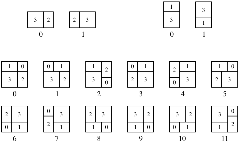
Note that we only consider rearrangements on the level of the tiles, and then always use the lower left corner of each prototile as marker or control point. Other choices are MLD with one of these, and do not change the spectral type (though they will lead to relatively translated windows in the cut and project description). Altogether, we thus obtain distinct inflation rules, all with the substitution matrix from Eq. (4.2). We parameterise the cases by triples with and . In particular, is the inflation from Eq. (4.1), while is the one from Eq. (5.1) and that of Eq. (5.4).
For each DPV, one can derive the window IFS in the same way as explained above. For precisely four choices of the parameters, namely , , and , one obtains the windows of Section 4 or a global translate thereof; see Figure 4. Observe that the inflation rules and emerge from by a reflection in the horizontal and vertical axis, respectively, and by applying both reflections. Since the original tiling hull is reflection symmetric, these four rules define the same hull. As a consequence of our convention to always choose the lower left corner as control point, which does not preserve the reflection symmetry, it turns out (after some calculations) that the resulting windows are related by global shifts. This in particular implies that these four DPVs share the same diffraction, namely the one illustrated in Figure 2.

Beyond these, there are another cases where the windows are parallelograms. They emerge from the original windows by shear transformations and shifts, as in the example (5.1) discussed previously. All vertices of the parallelograms are points in with simple coordinates. These cases are illustrated in Figure 5. The proof for each case consists in determining the window IFS followed by a verification that the corresponding set of quadrangles satisfies the IFS. We note that window systems with different slopes cannot produce projection point set that are MLD, as follows from an application of the general MLD criterion from [7, Rem. 7.6]. The window systems thus partition into MLD pairs, which are related by double reflections of the inflation rules, such as or .
Snapshots of the diffraction measures for the cases with horizontal window boundaries are shown in Figure 6. Let us make some brief comments on their structure, and that of the other cases. Directions in the Fourier module are mapped to directions in internal space under the -map, which is totally discontinuous. The directions of the ‘white streets’ (horizontal or vertical) are orthogonal to the vertical or horizontal edges of the windows. The second direction of the window boundaries shows up as a second direction in the intensity distributions, but in a less obvious way due to the complicated behaviour of the -map.


The remaining DPVs lead to windows of Rauzy fractal type. Rauzy fractals are compact sets that are topologically regular and perfect. Moreover, they have positive measure and a boundary of fractal (or Hausdorff) dimension less than that of ambient space, in this case ; see [21] for a summary of the general theory. For the Fibonacci DPVs, they come in three topological types, which we will call ‘castle’, ‘cross’ and ‘island’ to capture their geometric appearance.

After the preprint of our manuscript became available, Bernd Sing [22] calculated the Hausdorff dimensions of the three types of fractals. They all are of the form
where derives from the induced boundary IFS. It is the largest real root of a fractal-specific integer polynomial, namely
The corresponding three dimensions are approximately given by , and . It is clear from [7, Rem. 7.6] that projection sets with windows of different Hausdorff dimension cannot be MLD, which distinguishes the three types from one another, and also from all cases with polytopal windows.
There are four DPVs with windows of type ‘castle’ (left column of Figure 7). Two of them (the top ones) possess a reflection symmetry with respect to the diagonal, in the sense that the windows for the control points of the squares are symmetric, while the other two are interchanged. The remaining two DPV window systems form a -cycle under this reflection, with the corresponding exchange of the control points of the rectangular tiles. These relations between the DPVs can directly be extracted from the corresponding inflation rules as well.
The window systems of type ‘cross’ and ‘island’ are also shown in Figure 7. There are eight in each case, whose interrelations under reflections can be studied on the level of the inflation rules. Since the windows encode the control points, which are mapped to new positions under reflections, such reflections result in more complicated rearrangements of windows and parts of windows. An orbit analysis of the variations under rotations and reflections, as well as the ensuing classification into MLD classes, are left to the interested reader.
By an inspection analogous to the one that led to Proposition 5.1, it is clear that all these examples lead to regular model sets, some of which have windows with fractal boundaries. Each individual case comes with its characteristic internal Fourier matrix, which gives rise to the matrix function , where and are always the same, as is the Fourier module. Since , we can compute the FB amplitudes, and hence the diffraction, for all our examples via the internal cocycle. Due to the exponentially fast convergence of the cocycle product, the displayed results are free from numerical artefacts. Three examples are shown in Figure 8.
Theorem 5.2.
The inflation TDSs that emerge from the above DPVs all have pure point dynamical spectrum, namely . These systems are thus measure-theoretically isomorphic by the Halmos–von Neumann theorem. Each individual tiling, via the control points, leads to a Dirac comb with pure point diffraction measure.∎

It remains an interesting problem to understand the topological differences between the various DPV classes, which manifest themselves in different intensity distributions of the diffraction measures, or, equivalently, in different eigenfunctions for the (commuting) Koopman operators. In particular, while the examples of Figure 5 group into different MLD classes, it is plausible that they all are topologically conjugate to one another, and to the Fibonacci direct product TDS. In contrast, it is clear that the Rauzy fractal windows correspond to new classes under topological conjugacy, the details of which remain to be analysed.
The above analysis was illustrative, but is of exemplary type in the sense that it can be applied to any other Pisot substitution systems. In particular, while we chose planar examples for ease of presentability, the method works in higher dimensions as well. In view of the increasingly frequent appearance of Rauzy fractals as windows, the internal cocycle should prove to be a valuable tool to gain further insight. Its application is straightforward when the inflation factor is a unit, but becomes more delicate when it is not because the internal space is then no longer Euclidean; see [21] for the general framework required.
Acknowledgements
It is our pleasure to thank Lorenzo Sadun, Bernd Sing and Nicolae Strungaru for helpful discussions. MB is grateful to Manfred Denker for his encouragement to analyse geometric and spectral properties of tilings with methods from dynamical systems theory. We thank an anonymous referee for several thoughtful comments, which significantly helped to improve the presentation. This work was supported by the German Research Foundation (DFG), within the CRC 1283 at Bielefeld University, and by EPSRC through grant EP/S010335/1.
References
- [1] J. Aaronson, M. Denker, O. Sarig and R. Zweimüller, Aperiodicity of cocycles and conditional local limit theorems, Stoch. Dyn. 4 (2004) 31–62.
- [2] S. Akiyama, M. Barge, V. Berthé, J.-Y. Lee and A. Siegel, On the Pisot substitution conjecture, in Mathematics of Aperiodic Order, eds. J. Kellendonk, D. Lenz and J. Savinien (Birkhäuser, Basel, 2015) pp. 33–72.
- [3] M. Baake, M. Birkner and R.V. Moody, Diffraction of stochastic point sets: Explicitly computable examples, Commun. Math. Phys. 293 (2010) 611–660; arXiv:0803.1266.
- [4] M. Baake, N.P. Frank, U. Grimm and E.A. Robinson, Geometric properties of a binary non-Pisot inflation and absence of absolutely continuous diffraction, Studia Math. 247 (2019) 109–154; arXiv:1706.03976.
- [5] M. Baake and F. Gähler, Pair correlations of aperiodic inflation rules via renormalisation: Some interesting examples, Topology & Appl. 205 (2016) 4–27; arXiv:1511.00885.
- [6] M. Baake, F. Gähler and N. Mañibo, Renormalisation of pair correlation measures for primitive inflation rules and absence of absolutely continuous diffraction, Commun. Math. Phys. 370 (2019) 591–635; arXiv:1805.09650.
- [7] M. Baake and U. Grimm, Aperiodic Order. Vol. 1: A Mathematical Invitation (Cambridge University Press, Cambridge, 2013).
- [8] M. Baake and U. Grimm, Fourier transform of Rauzy fractals and point spectrum of 1D Pisot inflation tilings, preprint arXiv:1907.11012.
- [9] M. Baake and D. Lenz, Spectral notions of aperiodic order, Discr. Cont. Dynam. Syst. S 10 (2018) 161–190; arXiv:1601.06629.
- [10] M. Baake and R.V. Moody, Self-similar measures for quasicrystals, in Directions in Mathematical Quasicrystals, eds. M. Baake and R.V. Moody, CRM Monograph Series, vol. 13 (AMS, Providence, RI, 2000) pp. 1–42; arXiv:math.MG/0008063.
- [11] M. Denker, C. Grillenberger and K. Sigmund, Ergodic Theory of Compact Spaces, LNM 527 (Springer, Berlin, 1976).
- [12] M. Denker and M. Yuri, Conformal families of measures for general iterated function systems, in Recent Trends in Ergodic Theory and Dynamical Systems, eds. S. Bhattacharya, T. Das, A. Ghosh and R. Shah, Contemp. Math., vol. 631 (AMS, Providence, RI, 2015) pp. 93–108.
- [13] N.P. Frank, A primer of substitution tilings of the Euclidean plane, Expos. Math. 26 (2008) 295–326; arXiv:0705.1142.
- [14] N.P. Frank and E.A. Robinson, Generalized -expansions, substitution tilings, and local finiteness, Trans. Amer. Math. Soc. 360 (2008) 1163–1177; arXiv:math.DS/0506098.
- [15] B. Host, Valeurs propres des systèmes dynamiques définis par des substitutions de longueur variable, Ergodic Th. & Dynam. Syst. 6 (1986) 529–540.
- [16] J. Kellendonk and L. Sadun, Conjugacies of model sets, Discr. Cont. Dynam. Syst. A 37 (2017) 3805–3830; arXiv:1406.3851.
- [17] N. Mañibo, private communication (2019).
- [18] A.D. Pohl, Symbolic dynamics, automorphic functions, and Selberg zeta functions with unitary representations, in Dynamics and Numbers, eds. S. Kolyada, M. Möller, P. Moree and T. Ward, Contemp. Math., vol. 669 (AMS, Providence, RI, 2016) pp. 205–236; arXiv:1503.00525.
- [19] N. Pytheas Fogg, Substitutions in Dynamics, Arithmetics and Combinatorics, eds. V. Berthé, S. Ferenczi, C. Maduit and A. Siegel, LNM 1794 (Springer, Berlin, 2002).
- [20] M. Queffélec, Substitution Dynamical Systems — Spectral Analysis, 2nd ed., LNM 1294 (Springer, Berlin, 2010).
- [21] B. Sing, Pisot Substitutions and Beyond, PhD thesis (Bielefeld University, 2007); available electronically at urn:nbn:de:hbz:361-11555.
- [22] B. Sing, private communication (2019).
- [23] B. Solomyak, Dynamics of self-similar tilings, Ergodic Th. & Dynam. Syst. 17 (1997) 695–738 and Ergodic Th. & Dynam. Syst. 19 (1999) 1685 (Erratum).
- [24] N. Strungaru, private communication (2018).
- [25] B. Weiss, Single Orbit Dynamics, CBMS Regional Conference Series in Mathematics, vol. 95 (AMS, Providence, RI, 2000).