Scheduling Stochastic Real-Time Jobs
in Unreliable Workers Y.-P. Hsu, Y.-C. Huang, and S.-L. Shieh are with Department of Communication Engineering, National Taipei University, Taiwan. Email: {yupinhsu, ychuang, slshieh}@mail.ntpu.edu.tw. The work was supported by Ministry of Science and Technology of Taiwan under Grant MOST 107-2221-E-305-007-MY3.

Consider a distributed computing network consisting of a master and $M$ specialized workers $W_{1},\cdots,W_{M}$. The master is running $N$ applications $A_{1},\cdots,A_{N}$. Fig. 1 illustrates an example network with $N=2$ and $M=4$. Suppose that data transfer between the master and the workers occurs instantaneously with no error. Note that the prior works on the coflow model focused on the time for data transfer. To investigate the unreliability of the workers, we ignore the time for data transfer; instead, focus on the time for computation.

Divide time into frames and index them by $t=1,2,\cdots$. At the beginning of each frame $t$, each application stochastically generates a job, where a job is a collection of tasks that can be processed by the corresponding workers. Precisely, we use vector $\mathbf{J}_{i}(t)=(J_{i,1}(t),\cdots,J_{i,M}(t))$ to represent the job generated by application $A_{i}$ in frame $t$, where each element $J_{i,j}(t)\in\{0,1\}$ indicates if the job has a task for worker $W_{j}$: if $J_{i,j}(t)=1$, then the job $\mathbf{J}_{i}(t)$ has a task for worker $W_{j}$; otherwise, it does not. See Fig. 1 for example. Each task is also stochastically generated, i.e., $J_{i,j}(t)$ is a random variable for all $i$, $j$, and $t$. By $|\mathbf{J}_{i}(t)|$ we denote the number of 1’s in vector $\mathbf{J}_{i}(t)$; in particular, if $|\mathbf{J}_{i}(t)|=0$, then application $A_{i}$ generates no job in frame $t$. Suppose that the probability distribution of random variable $J_{i,j}(t)$ is independently and identically distributed (i.i.d.) over frame $t$, for all $i$ and $j$. Suppose that the tasks generated by application $A_{i}$ for worker $W_{j}$ have the same workload. See Remark 15 later for time-varying workloads. Moreover, the jobs need real-time computations. Suppose that the deadline for each job is one frame. The real-time system has been justified in the literature, e.g., see [13].

Consider a time-varying processing speed for each worker. Suppose that the processing speed of each worker is i.i.d. over frames. With the i.i.d. assumption along with those constant workloads, we can assume that a task generated by application $A_{i}$ can be completed by worker $W_{j}$ (i.e., when $J_{i,j}(t)=1$) with a constant probability $P_{i,j}$ over frames. At the end of each frame, each worker reports if its task is completed in that frame. A job is completed only when all its tasks are completed in the arriving frame. If any task of a job cannot be completed in the arriving frame, the job expires and is removed from the application.

Unaware of the completion of a task at the beginning of each frame, we suppose that the master assigns at most one task to a worker for each frame. If two jobs $\mathbf{J}_{i}(t)$ and $\mathbf{J}_{j}(t)$, for some $i$ and $j$, need the same worker in frame $t$, i.e., $J_{i,k}(t)=J_{j,k}(t)=1$ for some $k$, then we say the two jobs have interference. For example, jobs $\mathbf{J}_{1}(1)$ and $\mathbf{J}_{2}(1)$ in Fig. 1 have the interference.

As a result of the interference, the master has to decide a set of interference-free jobs for computing in each frame. Let $\mathbf{D}(t)\subseteq\{\mathbf{J}_{1}(t),\cdots,\mathbf{J}_{N}(t)\}$ be the set of interference-free jobs decided for computing in frame $t$. For example, decision $\mathbf{D}(1)$ in Fig. 1 can be either $\mathbf{J}_{1}(1)$ or $\mathbf{J}_{2}(1)$. If $\mathbf{D}(1)=\mathbf{J}_{1}(1)$ in Fig. 1, then workers $W_{1}$ and $W_{2}$ are allocated to job $\mathbf{J}_{1}(1)$ in frame $1$; moreover, job $\mathbf{J}_{1}(1)$ is completed only when the two workers complete their respective tasks in frame 1. A scheduling algorithm $\pi=\{\mathbf{D}(1),\mathbf{D}(2),\cdots\}$ is a time sequence of the decisions for all frames.

Let random variable $e_{i}(t;\pi)\in\{0,1\}$ indicate if job $\mathbf{J}_{i}(t)$ is completed in frame $t$ under scheduling algorithm $\pi$, where $e_{i}(t;\pi)=1$ if job $\mathbf{J}_{i}(t)$ is generated (i.e., $|\mathbf{J}_{i}(t)|\neq 0$) and all tasks of the job are completed by the corresponding workers in frame $t$; $e_{i}(t;\pi)=0$ otherwise. The random variable $e_{i}(t;\pi)$ depends on the random variables $J_{i,j}(t)$, the task completion probabilities $P_{i,j}$, and a potential randomized scheduling algorithm $\pi$.

We define the average number $\mathscr{N}_{i}(\pi)$ of completed jobs for application $A_{i}$ under scheduling algorithm $\pi$ by

Let vector $\mathbf{r}=(r_{1},\cdots,r_{N})$ represent an applications’ requirement for the average numbers of completed jobs. We say that requirement $\mathbf{r}$ can be fulfilled (or achieved) by scheduling algorithm $\pi$ if $\mathscr{N}_{i}(\pi)\geq r_{i}$ for all $i$. Moreover, we refer to requirement $\mathbf{r}$ as a feasible requirement if there exists a scheduling algorithm that can fulfill the requirement. We define the maximum feasibility region as follows.

We define an optimal scheduling algorithm as follows.

The goal of this paper is to devise a feasibility-optimal scheduling algorithm.

Given the distributed computing network with scheduling algorithm $\pi$ and requirement $\mathbf{r}$, we construct a virtual queueing network. The virtual queueing network consists of $N$ queues $Q_{1},\cdots,Q_{N}$, operating under the same frame system as that in Section II-A. For example, Fig. 2 is the virtual queueing network for the distributed computing network in Fig. 1. We want to emphasize that the virtual queueing network is not a real-world network. It is introduced for the scheduling design in Section III-B.

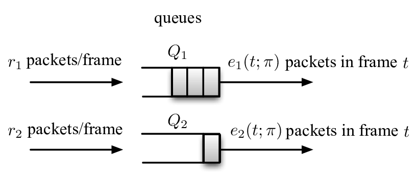
At the beginning of each frame $t$, a fixed number³³ 3 The virtual queueing network has a fractional number of packets. $r_{i}$ of packets arrive at queue $Q_{i}$. At the end of frame $t$, queue $Q_{i}$ can remove $e_{i}(t;\pi)$ packet, i.e., if job $\mathbf{J}_{i}(t)$ is completed in frame $t$, then queue $Q_{i}$ can remove one packet at the end of frame $t$; otherwise, it removes no packet in frame $t$. Again, note that those packets are not real-world packets. We summarize the packet arrival rate and the packet service rate as follows.

Let $Q_{i}(t)$ be the queue size at queue $Q_{i}$ at the beginning (before new packet arrival) of frame $t$. Then, the queueing dynamics of queue $Q_{i}$ can be expressed by $Q_{i}(t+1)=\max\{Q_{i}(t)+r_{i}-e_{i}(t;\pi),0\}$. Let $\mathbf{Q}(t)=(Q_{1}(t),\cdots,Q_{N}(t))$ be the vector of all queue sizes at the beginning of frame $t$. We define the notion of a stable queue in Definition 4, followed by introducing a necessary condition for the stable queue in Proposition 5.

By Propositions 3 and 5, we can turn our attention to developing a scheduling algorithm such that, for any requirement $\mathbf{r}$ interior of $\mathbf{R}_{\max}$, all queues in the virtual queueing network are stable.

We want to emphasize that, unlike traditional stochastic networks (e.g., [14, 13]), each packet in our virtual queueing network can be removed only when all associated tasks are completed in its arriving frame. Thus, our paper generalizes to stochastic networks with multiple required servers; in particular, we develop a tractable approximate scheduling algorithm for the scenario in Section III-C.

In this section, we propose a feasibility-optimal scheduling algorithm in Alg. 1. At the beginning of frame 1, Alg. 1 (in Line 1) initializes all queue sizes to be zeros. At the beginning of each frame $t$, Alg. 1 (in Line 1) updates each queue $Q_{i}$ with the new arriving $r_{i}$ packets; then, Alg. 1 (in Line 1) decides $\mathbf{D}(t)$ for that frame according to the present queue size vector $\mathbf{Q}(t)$. The decision $\mathbf{D}(t)$ is made for maximizing the weighted sum of the queue sizes in Eq. (2). The term $\mathbf{1}_{|\mathbf{J}_{i}(t)|\neq 0}\cdot\prod_{j:J_{i,j}(t)=1}P_{i,j}$ in Eq. (2) calculates the expected packet service rate for $Q_{i}$, where the indicator function $\mathbf{1}_{|\mathbf{J}_{i}(t)|\neq 0}$ indicates if job $\mathbf{J}_{i}(t)$ is generated in frame $t$, and if so, that job can be completed with probability $\prod_{j:J_{i,j}(t)=1}P_{i,j}$. The underlying idea of Alg. 1 is to remove as many packets from the virtual queueing network as possible (for stabilizing all queues).

After performing the decision $\mathbf{D}(t)$, Alg. 1 (in Line 1) updates each $Q_{i}$ at the end of frame $t$: if job $\mathbf{J}_{i}(t)$ is scheduled, the job is indeed generated, and all its required workers complete their respective tasks, then one packet is removed from queue $Q_{i}$ in the virtual queuing network.

Leveraging Lyapunov techniques [14], we can establish the optimality of Alg. 1 in the following.

Note that Alg. 1 involves a combinatorial optimization problem in Line 1. In the next section, we will investigate the computational complexity for solving the combinatorial optimization problem.

We show (in the next lemma) that the combinatorial optimization problem in Line 1 of Alg. 1 is NP-hard. Therefore, Alg. 1 is computationally intractable.

To study the NP-hard problem, we define two notions of approximation ratios as follows. While Definition 9 studies the resulting value in Eq. (2), Definition 10 investigates the resulting region of achievable requirements.

In this paper, we propose an approximate scheduling algorithm in Alg. 2. The procedure of Alg. 2 is similar to that of Alg. 1; hence, we point out key differences in the following.

Unlike Alg. 1 solving the combinatorial optimization problem, Alg. 2 (in Line 2) simply sorts all jobs according to the values computed by Eq. (10). Let $\mathbf{J}^{(1)}(t),\cdots,\mathbf{J}^{(N)}(t)$ (in Line 2) denote the sorted jobs in frame $t$ in descending order of the values from Eq. (10). In addition, let $J^{(i)}_{j}(t)$ (in Line 2) indicate if job $\mathbf{J}^{(i)}$ has a task for worker $W_{j}$ in frame $t$. While the numerator of Eq. (10) indicates the weight $Q_{i}(t)\prod_{j:J_{i,j}(t)=1}P_{i,j}$ in Eq. (2) for job $\mathbf{J}_{i}(t)$, the denominator of that reflects the maximum number of jobs interfered by job $\mathbf{J}_{i}(t)$. The underlying idea of Alg. 2 is to consider jobs in $\mathbf{J}^{(1)}(t),\cdots,\mathbf{J}^{(N)}(t)$ order, for achieving a higher value of Eq. (2) and at the same time keeping the interference as low as possible.

More precisely, Alg. 2 uses a set $\mathbf{U}$ to record (in Line 2) the available workers that are not allocated yet, where set $U$ is initialized to be $\{W_{1},\cdots,W_{M}\}$ in Line 2. Then, at the $i$-th iteration of Line 2, Alg. 2 checks if job $\mathbf{J}^{(i)}(t)$ satisfies the two conditions in Line 2: the first condition $|\mathbf{J}^{(i)}(t)|\neq 0$ means that job $\mathbf{J}_{i}(t)$ is generated and the second condition $\{W_{j}:J^{(i)}_{j}(t)=1\}\subseteq\mathbf{U}$ means that its required workers are all available. If job $\mathbf{J}^{(i)}(t)$ meets the conditions, then it is scheduled as in Line 2. In addition, if job $\mathbf{J}^{(i)}(t)$ is scheduled, then set $\mathbf{U}$ is updated as in Line 2 by removing the workers allocated to job $\mathbf{J}^{(i)}(t)$. After deciding $\mathbf{D}(t)$, Alg. 2 performs the decision $\mathbf{D}(t)$ in Line 2 for frame $t$, followed by updating the queue sizes in Line 2.

Next, we establish the approximation ratio of Alg. 2 to Eq. (2).

With Lemma 12, we can further establish the approximation ratio of Alg. 2 to $\mathbf{R}_{\max}$.

The computational complexity of Alg. 2 is $O(\log N)$ primarily caused by sorting all queues in Line 2. Thus, Alg. 2 is tractable when the number of applications is large.

References

- [1] J. Dean and S. Ghemawat, “MapReduce: Simplified Data Processing on Large Clusters,” Communications of the ACM, vol. 51, no. 1, pp. 107–113, 2008.
- [2] A. Tveit, Ø. Rein, J. V. Iversen, and M. Matskin, “Scalable Agent-Based Simulation of Players in Massively Multiplayer Online Games,” Proc. of SCAI, p. 80–89.
- [3] M. Chowdhury and I. Stoica, “Coflow: A Networking Abstraction for Cluster Applications.” Proc. of ACM HotNets, pp. 31–36, 2012.
- [4] M. Chowdhury, Y. Zhong, and I. Stoica, “Efficient Coflow Scheduling with Varys,” Proc. of ACM SIGCOMM, vol. 44, no. 4, pp. 443–454, 2014.
- [5] Y. Li, S. H.-C. Jiang, H. Tan, C. Zhang, G. Chen, J. Zhou, and F. Lau, “Efficient Online Coflow Routing and Scheduling,” Proc. of ACM MobiHoc, pp. 161–170, 2016.
- [6] M. Shafiee and J. Ghaderi, “An Improved Bound for Minimizing the Total Weighted Completion Time of Coflows in Datacenters,” IEEE/ACM Trans. Netw., vol. 26, no. 4, pp. 1674–1687, 2018.
- [7] S.-H. Tseng and A. Tang, “Coflow Deadline Scheduling via Network-Aware Optimization,” Proc. of Allerton, pp. 829–833, 2018.
- [8] S. Im, B. Moseley, K. Pruhs, and M. Purohit, “Matroid Coflow Scheduling,” Proc. of ICALP, pp. 1–14, 2019.
- [9] S. Wang, J. Zhang, T. Huang, J. Liu, T. Pan, and Y. Liu, “A Survey of Coflow Scheduling Schemes for Data Center Networks,” IEEE Commun. Mag., vol. 56, no. 6, pp. 179–185, 2018.
- [10] G. Ananthanarayanan, A. Ghodsi, S. Shenker, and I. Stoica, “Effective Straggler Mitigation: Attack of the Clones,” Proc. of NSDI, pp. 185–198, 2013.
- [11] Q. Liang and E. Modiano, “Coflow Scheduling in Input-Queued Switches: Optimal Delay Scaling and Algorithms,” Proc. of IEEE INFOCOM, pp. 1–9, 2017.
- [12] B. Li, Z. Shi, and A. Eryilmaz, “Efficient Scheduling for Synchronized Demands in Stochastic Networks,” Proc. of IEEE WiOpt, pp. 1–8, 2018.
- [13] I.-H. Hou and P. R. Kumar, Packets with Deadlines: A Framework for Real-Time Wireless Networks. Morgan & Claypool Publishers, 2013, vol. 6, no. 1.
- [14] M. J. Neely, Stochastic Network Optimization with Application to Communication and Queueing Systems. Morgan & Claypool Publishers, 2010, vol. 3, no. 1.
- [15] L. Georgiadis, M. J. Neely, and L. Tassiulas, Resource Allocation and Cross-Layer Control in Wireless Networks. Now Publishers, Inc., 2006, vol. 1, no. 1.
- [16] M. M. Halldórsson, J. Kratochvíl, and J. A. Telle, “Independent Sets with Domination Constraints,” Proc. of ICALP, pp. 176–187, 1998.
- [17] K. Lee, M. Lam, R. Pedarsani, D. Papailiopoulos, and K. Ramchandran, “Speeding Up Distributed Machine Learning using Codes,” IEEE Trans. Inf. Theory, vol. 64, no. 3, pp. 1514–1529, 2017.
- [18] C.-S. Yang, R. Pedarsani, and A. S. Avestimehr, “Timely-Throughput Optimal Coded Computing over Cloud Networks,” Proc of ACM MobiHoc, pp. 301–310, 2019.