Fast integral equation methods for linear and semilinear heat equations in moving domains

J. Wang¹ L. Greengard2 3] S. Jiang⁴ S. Veerapaneni⁵ Affiliation: Affiliation: ¹Yau Mathematical Sciences Center,
Tsinghua University,
Haidian District, Beijing, China 100084 Affiliation: Email: jwang2020@tsinghua.edu.cn Affiliation: Affiliation: ²Flatiron Institute, Simons Foundation,
New York, New York 10010 Affiliation: ³Courant Institute, New York University,
New York, New York 10012 Affiliation: Email: greengard@courant.nyu.edu Affiliation: Affiliation: ⁴Department of Mathematics Sciences,
New Jersey Institute of Technology,
Newark, New Jersey 07102 Affiliation: Email: shidong.jiang@njit.edu Affiliation: Affiliation: ⁵Department of Mathematics, University of Michigan,
Ann Arbor, Michigan 48109 Affiliation: Email: shravan@umich.edu

Abstract

We present a family of integral equation-based solvers for the linear or semilinear heat equation in complicated moving (or stationary) geometries. This approach has significant advantages over more standard finite element or finite difference methods in terms of accuracy, stability and space-time adaptivity. In order to be practical, however, a number of technical capabilites are required: fast algorithms for the evaluation of heat potentials, high-order accurate quadratures for singular and weakly integrals over space-time domains, and robust automatic mesh refinement and coarsening capabilities. We describe all of these components and illustrate the performance of the approach with numerical examples in two space dimensions.

1 Introduction

A variety of problems in applied physics, chemistry and engineering require the solution of the diffusion equation

\begin{split}u_{t}({\bf x},t)&=\Delta u({\bf x},t)+F(u,{\bf x},t),\\ u({\bf x},0)&=u_{0}({\bf x}),\end{split}

(1)

for $t>0$ and ${\bf x}\in\mathbb{R}^{d}$ . The problem is sometimes posed in free space, but often it is assumed that $({\bf x},t)$ lies in the interior or exterior of a space-time domain

\Omega_{T}=\prod_{0}^{T}\Omega(t)\subset\mathbb{R}^{d}\times(0,T],

(2)

subject to suitable conditions on its boundary

\Gamma_{T}=\prod_{0}^{T}\Gamma(t),

(3)

where $\Gamma(t)=\partial\Omega(t)$ . As a matter of nomenclature, we refer to the equation (1) as semilinear and nonautonomous. When $F(u,{\bf x},t)=F(u)$ , the equation is autonomous, and when $F(u,{\bf x},t)=F({\bf x},t)$ , it is linear.

Classical methods, such as finite difference or finite element methods, evolve the solution at successive time steps, using some local approximation of the partial differential equation (PDE) (1) itself. While more general, they are known to have a severe constraint on the size of time step when relying on an explicit marching scheme. Using the forward Euler method, for example, if we approximate the Laplacian via the second order central difference operator on a uniform grid with the same spacing in each coordinate direction, then the stability condition for solving the pure initial value problem requires that $\Delta t\leq\frac{1}{2d}\Delta x^{2}$ , where $\Delta t$ is the time step, $\Delta x$ is the step in the spatial discretization, and $d$ is the ambient dimension. In general, the stability constraint takes the form ${\Delta t}=\mathcal{O}(h^{2})$ where $h$ is the smallest spacing in the spatial discretization. This constraint is typically overcome by using an implicit marching scheme. Even in the linear case, however, this involves the solution of a system of algebraic equations at each time step, coupling all the spatial grid points. In the semilinear case, it requires the solution of a large, nonlinear system of equations. Moreover, high order accuracy is difficult to achieve with direct discretization methods when dealing with time-dependent domains. The available literature on such approaches is vast and we do not seek to review it here. In this paper, we focus on the use of parabolic potential theory [11, 19, 30, 61] and the development of the fast algorithms that will permit us to solve fairly general initial-boundary value problems.

Let us first consider the linear setting, when the forcing term $F(u,{\bf x},t)=F({\bf x},t)$ in (1) is known, in the absence of physical boundaries. For the sake of simplicity, we assume that the forcing term at time $t$ is supported in the bounded domain $\Omega(t)$ and that the initial data $u_{0}({\bf x})$ is supported in $\Omega(0)$ . This is a well-posed problem in free space under mild conditions on the behavior of $u$ at infinity [19, p. 25]. The solution to (1) can be expressed at any later time $t$ in closed form as

u^{(V)}({\bf x},t)=\mathcal{I}[u_{0}]({\bf x},t)+\mathcal{V}[F]({\bf x},)

(4)

with

\mathcal{I}[u_{0}]({\bf x},t)=\int_{\Omega(0)}G({\bf x}-{\bf y},t)u_{0}({\bf y})\,d{\bf y},

(5)

and

\mathcal{V}[F]({\bf x},t)=\int_{0}^{t}\int_{\Omega(\tau)}G({\bf x}-{\bf y},t-\tau)F({\bf y},\tau)\,d{\bf y}d\tau.

(6)

Here,

G({\bf x},t)=\frac{e^{-\|{\bf x}\|^{2}/4t}}{(4\pi t)^{d/2}}

(7)

is the free-space Green’s function for the heat equation (the heat kernel) in $d$ dimensions, The functions $\mathcal{I}[u_{0}]$ and $\mathcal{V}[F]$ are referred to as initial and volume (heat) potentials, respectively.

Remark 1.1.

The spatial domains of integration in $\mathcal{I}[u]({\bf x},t)$ and $\mathcal{V}[F]({\bf x},t)$ are implicitly assumed to be the support of the indicated functions. Above, these are finite domains defined by $\Omega(0)$ and $\Omega_{t}$ , respectively.

Remark 1.2.

In the remainder of this paper, we will assume $d=2$ .

A compelling feature of the solution $u^{(V)}$ is that it is exact, explicit, and does not involve the inversion of any matrices. It requires only the evaluation of the initial and volume potentials. Thus, stability never arises as an issue, and the error is simply the quadrature error in approximating the integral operators in the relevant potentials themselves. This approach is typically ignored for two simple reasons. First, good quadrature rules are needed and second, in the absence of fast algorithms, the computational cost is excessive. More precisely, assuming there are $N_{T}$ time steps, $N$ points in the discretization of $F$ and $N$ target points at each time step, naive summation applied to (6) requires $O(N^{2}N_{T}^{2})$ work.

For a time step $\Delta t$ , however, using the definition of the heat kernel, it is straightforward to see that

	$\displaystyle u^{(V)}({\bf x},t+\delta)=$	$\displaystyle\int_{\mathbb{R}^{d}}G({\bf x}-{\bf y},\delta)\,u^{(V)}({\bf y},t)\,d{\bf y}+$		(8)
		$\displaystyle\int_{t}^{t+\delta}\int_{\Omega(\tau)}G({\bf x}-{\bf y},t+\delta-\tau)\,F({\bf y},\tau)\,d{\bf y}d\tau.$		(8)

That is to say, the heat equation in free space can be solved by sequential convolution with the heat kernel at every time step, followed by the addition of a local contribution from the forcing term $F({\bf x},t)$ over the last time step alone. This is simply the semigroup property satisfied by the heat equation itself, and can be viewed as a marching scheme for the PDE expressed in integral form. Using this approach, the apparent history-dependence of evaluating heat potentials has vanished and the net cost has dropped from $O(N^{2}N_{T}^{2})$ to $O(N^{2}N_{T})$ work, assuming some suitable quadrature rule has been developed for the integrals in (8). There is, however, a small catch. Note that the first spatial integral in (8) is of the form

\mathcal{I}[u^{(V)}({\bf x},t)]({\bf x},t+\delta)=\int_{\mathbb{R}^{d}}G({\bf x}-{\bf y},\delta)u^{(V)}({\bf y},t)\,d{\bf y},

with the domain of integration $\mathbb{R}^{d}$ , whereas the domain of integration in the exact solution (4) is the bounded region $\Omega_{t}$ - the support of the data itself. Thus, in order to make use of the marching scheme (8), we will have to cope with the spreading of the solution in free space over time. This turns out to be surprisingly easy to do (see section 3).

In many applications, physical boundaries are present on which additional conditions are imposed. We will limit our attention to three standard boundary value problems. For the Dirichlet problem, the value of the solution on the boundary is given:

u({\bf x},t)=f({\bf x},t)\qquad({\bf x},t)\in\Gamma_{T}.

(9)

For the Neumann problem, the value of the normal derivative of the solution at the boundary is given:

\frac{\partial u}{\partial\nu_{{\bf x}}}({\bf x},t)=g({\bf x},t)\quad({\bf x},t)\in\Gamma_{T},

(10)

where $\nu_{{\bf x}}$ denotes the normal vector at the boundary point ${\bf x}$ . For the Robin problem, a specific linear combination of the solution and its normal derivative is given on the boundary:

\frac{\partial}{\partial\nu_{{\bf x}}}u({\bf x},t)+\alpha({\bf x},t)u({\bf x},t)=h({\bf x},t)\qquad({\bf x},t)\in\Gamma_{T},

(11)

with $\alpha({\bf x},t)\geq 0$ .

In standard finite difference and finite element methods, the boundary condition must be coupled with the interior marching scheme, which can impose additional stability constraints on the time step [31, 32, 60, 69, 75]. In the framework of potential theory, on the other hand, we may write the solution to the full (linear) initial-boundary value problem as

u=u^{(V)}+u^{(B)},

(12)

where $u^{(V)}$ is given by (4) and $u^{(B)}$ is the solution to a homogeneous boundary value problem with zero initial data and no forcing term. The boundary condition for $u^{(B)}$ is simply the original boundary condition for $u({\bf x},t)$ , from which is subtracted the contribution of $u^{(V)}$ . We will see below that we can represent $u^{(B)}$ in terms of layer heat potentials defined in terms of unknown densities which are restricted to the space-time boundary $\Gamma_{T}$ . These densities are determined by the boundary data through the solution of Volterra integral equations of the second kind. This formulation has some remarkable benefits. First, explicit marching schemes are not subject to a mesh-dependent stability constraint. In fact, for the Dirichet and Neumann problems, they can be unconditionally stable, as discussed in section 4. Second, integral equations are naturally compatible with moving boundaries, and apply equally well to interior or exterior problems. In the latter case, they do not require the artificial truncation of the computational domain or the associated difficulties in constructing suitable “outgoing” boundary conditions. As for the volume potential discussed above, however, there are two principal drawbacks to making such computations practical: the exhorbitant computational cost and the need to integrate singular or weakly singular kernels over complicated surfaces in space-time. A naive algorithm would again require an amount of work of the order $\mathcal{O}(NN_{S}N_{T}^{2})$ where $N$ is the number of target points at each time step, $N_{S}$ is the number of discretization points on the boundary $\Gamma(t)$ and $N_{T}$ is the number of time steps.

1.1 Semilinear problems

For the full, non-autonomous semilinear problem (1) in free space, we may still use the representation (4), but now

\mathcal{V}[F]({\bf x},t)=\int_{0}^{t}\int_{\Omega(\tau)}G({\bf x}-{\bf y},t-\tau)F(u,{\bf y},\tau)\,d{\bf y}d\tau.

(13)

This still permits the analog of the marching scheme (8), except that

	$\displaystyle u({\bf x},t+\delta)=$	$\displaystyle\int_{\mathbb{R}^{d}}G({\bf x}-{\bf y},\delta)u({\bf y},t)\,d{\bf y}\ +$		(14)
		$\displaystyle\int_{t}^{t+\delta}\int_{\Omega(\tau)}G({\bf x}-{\bf y},t+\delta-\tau)F(u,{\bf y},\tau)\,d{\bf y}d\tau.$		(14)

is now a nonlinear integral equation for $u({\bf x},t)$ rather than an explicit, exact solution. We discuss the solution to such problems in section 5.

1.2 Periodic boundary conditions

In many applications, the solution of the heat equation is required with periodic boundary conditions on, say, the unit box $B=[-\frac{1}{2},\frac{1}{2}]\times[-\frac{1}{2},\frac{1}{2}]$ . That is, $u({\bf x},t)$ must satisfy

	$\displaystyle u(-\tfrac{1}{2},y)$	$\displaystyle=u(\tfrac{1}{2},y),\quad u_{x}(-\tfrac{1}{2},y)=u_{x}(\tfrac{1}{2},y),\ {\rm for}\ -\tfrac{1}{2}\leq y\leq\tfrac{1}{2}$
	$\displaystyle u(x,-\tfrac{1}{2})$	$\displaystyle=u(x,\tfrac{1}{2}),\quad u_{y}(x,-\tfrac{1}{2})=u_{y}(x,\tfrac{1}{2}),\ {\rm for}\ -\tfrac{1}{2}\leq x\leq\tfrac{1}{2}.$

In the absence of physical boundaries, the solution to the linear heat equation with forcing is again of the form (4), but with $G({\bf x},t)$ defined to be the periodic Green’s function for the heat equation in two dimensions:

G_{P}({\bf x},t)=\sum_{j=-\infty}^{\infty}\sum_{k=-\infty}^{\infty}\frac{e^{-\|{\bf x}+(j,k)\|^{2}/4t}}{(4\pi t)},

(15)

using the method of images. The marching scheme in (8) still applies, except the domain of integration is the box $B$ for both the initial potential and the local increment, rather than ${\mathbb{R}^{2}}$ and $\Omega(t)$ . Moreover, the marching scheme (14) applies in the semilinear case here as well (with $G_{P}({\bf x},t)$ replacing the free space Green’s function $G({\bf x},t)$ ).

We will also consider boundary value problems where a collection of inclusions define a region $\Omega_{T}\subset B$ , and the domain of interest is the complement $B\setminus\Omega_{T}$ , with periodic conditions on $B$ and Dirichlet, Neumann or Robin conditions on $\Gamma_{T}$ (see Section 6).

Figure 1: Typical domains of interest: on the left is a multiply connected region defined by the closed curves

\Gamma_{1}(t),\dots,\Gamma_{M}(t)

. Interior problems include an outer boundary

\Gamma_{0}(t)

and the domain defined at time

t

\Gamma(t)=\cup_{i=0}^{M}\Gamma_{i}(t)

. We will also consider boundary value problems in the exterior domain bounded at time

t

\Gamma(t)=\cup_{i=1}^{M}\Gamma_{i}(t)

. Periodic boundary value problems are illustrated on the right. We show the unit box

B

and its eight nearest neighbors in an infinite tiling of the plane. When inclusions are present, the domain of interest is

B\setminus\Omega_{T}

, where

\Omega_{T}

is the region bounded by the indicated curves. We will also consider periodic problems in the absence of inclusions, defined by initial data and a linear or semilinear forcing term.

1.3 Synopsis of the paper

The paper is organized as follows. In section 2, we review the relevant parts of parabolic potential theory and show how to reformulate the various boundary value problems as Volterra integral equations of the second kind. In section 3 and 3.9.1, we discuss the state of the art in fast algorithms for the evaluation of heat potentials, focusing on some recently developed quadrature methods and adaptive versions of the fast Gauss transform (FGT) [7, 28, 27, 29, 24, 45, 49, 63, 65, 67, 70, 79, 83]. The full numerical scheme for boundary value problems is summarized in section 5, and extensive numerical examples are provided in section 6 in both the linear and semilinear settings. We conclude in section 7 with a discussion of open problems.

We hope to make clear some of the distinct advantages to be gained from using the integral equation framework. These include the following:

1.

Explicit marching schemes, as mentioned above, can be unconditionally stable (see section 4).
2.

For semilinear problems, fully implicit methods require only the solution of scalar nonlinear equations [16], unlike PDE-based methods (see section 5).
3.

Fast algorithms are available with which all of the methods described are asymptotically optimal and able to achieve arbitrary order accuracy (see section 3).

1.4 Notation

In the table below, we list some symbols that will be used frequently.

Symbol	Definition
$\Omega_{T}$	Space-time domain (eq. 2)
$\Gamma_{T}$	Space-time boundary (eq. 3)
$\mathcal{I}$	Initial potential (eq. 5)
$\mathcal{V}$	Volume potential (eq. 6)
$\mathcal{S}$	Single-layer potential (eq. 17)
$\mathcal{D}$	Double-layer potential (eq. 18)
$\mathcal{S}_{H},\mathcal{D}_{H},\mathcal{V}_{H}$	the history parts of $\mathcal{S}$ , $\mathcal{D}$ and $\mathcal{V}$ (eq. 39)
$\mathcal{S}_{NH},\mathcal{D}_{NH}$	the near history parts of $\mathcal{S}$ and $\mathcal{D}$ (eq. 67)
$\mathcal{S}_{FH},\mathcal{D}_{FH}$	the far history parts of $\mathcal{S}$ and $\mathcal{D}$ (eq. 68)
$\mathcal{S}_{L},\mathcal{D}_{L},\mathcal{V}_{L}$	the local parts of $\mathcal{S}$ , $\mathcal{D}$ and $\mathcal{V}$ (eq. 40)
$\mathcal{S}_{\epsilon},\mathcal{D}_{\epsilon}$	the asymptotic parts of $\mathcal{S}$ and $\mathcal{D}$ (eq. 71)

Table 1: Index of frequently used symbols and operators.

2 Mathematical Preliminaries

In this section, we review classical potential theory for the heat equation and refer the reader to the texts [19], [30], and [61] for more thorough treatments. While the theory is similar to that for the elliptic case (governed by the Laplace or Helmholtz equations), there are some important differences. Existence and uniqueness results are easier to obtain because the integral equations that arise are second kind Volterra equations rather than Fredholm equations, avoiding the possibility of spurious resonances.

As noted in the introduction, it is well-known that the equations (1) are well-posed in free space, with the solution given by (4). The solution is unique assuming $u_{0}({\bf x})$ and $F({\bf x},t)$ are continuous and bounded by some constant $L$ on ${\mathbb{R}}^{d}$ [19, 61]. In that case, the solution $u^{(V)}({\bf x},t)$ to (1) is continuous and satisfies $|u^{(V)}({\bf x},t)|\leq L$ for ${\bf x}\in{\mathbb{R}}^{d}$ and $t>0$ .

2.1 The classical initial-boundary value problems

We turn now to a consideration of interior boundary value problems in domains $\Omega_{T}$ or their exterior counterparts, defined in $\Omega_{T}^{c}=\prod_{t=0}^{T}\Omega^{c}(t)$ , where $\Omega^{c}(t)={\mathbb{R}}^{d}\backslash\Omega(t)$ , as depicted in Fig. 1. When the spatial domain is stationary, we will denote the space-time domain on which the heat equation is to be solved by the interior region $\Omega_{T}=\Omega\times[0,T]$ , with boundary $\Gamma_{T}=\Gamma\times[0,T]$ and the corresponding exterior domain as $\Omega_{T}^{c}$ . As indicated earlier, we denote the unit outward normal to $\Gamma(t)$ at each point ${\bf x}\in\Gamma(t)$ by $\nu_{{\bf x}}$ and the positively-oriented unit tangent vector at ${\bf x}$ by $\tau_{{\bf x}}$ . For all boundary value problems of interest, we assume that

	$\displaystyle u_{t}({\bf x},t)$	$\displaystyle=\Delta u({\bf x},t)+F({\bf x},t),\qquad({\bf x},t)\in\Omega_{T},$		(16)
	$\displaystyle u({\bf x},0)$	$\displaystyle=u_{0}({\bf x}),\qquad{\bf x}\in\overline{\Omega(0)}.$		(16)

For the sake of simplicity, we always assume that the initial and boundary data are compatible. For the Dirichlet problem, where we impose (9), this requires that

f({\bf x},0)=u_{0}({\bf x}),\qquad{\bf x}\in\Gamma(0).

For the Neumann problem, where we impose (10), this requires that

g({\bf x},0)=\frac{\partial}{\partial\nu_{{\bf x}}}u_{0}({\bf x}),\qquad{\bf x}\in\Gamma(0).

Finally, for the Robin problem, where we impose (11), this requires that

h({\bf x},0)=\frac{\partial}{\partial\nu_{{\bf x}}}u_{0}({\bf x})+\alpha({\bf x})u_{0}({\bf x}),\qquad{\bf x}\in\Gamma(0).

2.2 Layer Heat Potentials

As in the elliptic case, homogeneous partial differential equations of parabolic type can be reduced to boundary integral equations when the material coefficients (here the conductivities) are constant. This transformation makes essential use of the governing Green’s function and a source distribution restricted to the space-time boundary $\Gamma_{T}$ , called a surface density or layer potential density. Formally speaking, these are distributions when viewed as functions in the ambient space (like a surface charge or surface current density in electromagnetic theory) but simply defined as functions on the surface using a suitable parametrization.

Definition 1.

In the remainder of this paper, we assume the domain $\Omega_{T}$ is sufficiently smooth, meaning that the domain boundary $\Gamma(t)$ is $C^{2}$ with continuous curvature and that, in the moving geometry case, it evolves with a continuous velocity.

Definition 2.

Suppose that $\Omega_{T}$ is a sufficiently smooth, bounded space-time domain and that the single and double layer densities $\sigma({\bf x},t)$ and $\mu({\bf x},t)$ are continuous for $({\bf x},t)\in\Gamma_{T}$ . Then, the single layer potential $\mathcal{S}[\sigma]$ is given by

\mathcal{S}[\sigma]({\bf x},t)=\int_{0}^{t}\int_{\Gamma(\tau)}G({\bf x}-{\bf y},t-\tau)\sigma({\bf y},\tau)ds_{{\bf y}}d\tau,

(17)

and the double layer potential $\mathcal{D}[\mu]$ is given by

\mathcal{D}[\mu]({\bf x},t)=\int_{0}^{t}\int_{\Gamma(\tau)}\frac{\partial}{\partial\nu_{{\bf y}}}G({\bf x}-{\bf y},t-\tau)\mu({\bf y},\tau)ds_{{\bf y}}d\tau\,.

(18)

The layer heat potentials defined in (17) and (18) satisfy well-known jump conditions as ${\bf x}$ approaches a point ${\bf x}_{0}$ on the boundary $\Gamma(t)$ from either the interior or exterior. Their derivations are standard [19, 30, 61] and easily deduced from their better known elliptic analogs.

Theorem 2.1.

The single layer potential $\mathcal{S}[\sigma]({\bf x},t)$ is continuous for all ${\bf x}\in{\mathbb{R}}^{2}$ and $t\geq 0$ and satisfies the relations

	$\displaystyle\frac{\partial}{\partial t}\mathcal{S}[\sigma]({\bf x},t)=\Delta\mathcal{S}[\sigma]({\bf x},t),\;\;\;x\notin\Gamma(t),\;\;\;t>0,$		(19)
	$\displaystyle\mathcal{S}[\sigma]({\bf x},0)=0,\;\;\;x\notin\Gamma(t),$		(20)
	$\displaystyle\lim_{\begin{subarray}{c}{\bf x}\rightarrow{\bf x}_{0}\in\Gamma(t)\\ {\bf x}\in\Omega(t)\end{subarray}}\frac{\partial}{\partial\nu_{{\bf x}_{0}}}\mathcal{S}[\sigma]({\bf x},t)=\frac{1}{2}\sigma({\bf x}_{0},t)+\frac{\partial}{\partial\nu_{{\bf x}_{0}}}\mathcal{S}[\sigma]({\bf x}_{0},t),$		(21)
	$\displaystyle\lim_{\begin{subarray}{c}{\bf x}\rightarrow{\bf x}_{0}\in\Gamma(t)\\ {\bf x}\in\Omega^{c}(t)\end{subarray}}\frac{\partial}{\partial\nu_{{\bf x}_{0}}}\mathcal{S}[\sigma]({\bf x},t)=-\frac{1}{2}\sigma({\bf x}_{0},t)+\frac{\partial}{\partial\nu_{{\bf x}_{0}}}\mathcal{S}[\sigma]({\bf x}_{0},t)\,,$		(22)

where the expression $\frac{\partial}{\partial\nu_{{\bf x}_{0}}}\mathcal{S}[\sigma]({\bf x}_{0},t)$ is interpreted in the principal value sense.

Theorem 2.2.

The double layer potential $\mathcal{D}[\mu]({\bf x},t)$ is defined for all ${\bf x}\in{\mathbb{R}}^{d}$ and $t\geq 0$ and satisfies the relations

	$\displaystyle\frac{\partial}{\partial t}\mathcal{D}[\mu]({\bf x},t)=\Delta\mathcal{D}[\mu]({\bf x},t),\;\;\;x\notin\Gamma(t),\;\;\;t>0,$		(23)
	$\displaystyle\mathcal{D}[\mu]({\bf x},0)=0,\;\;\;x\notin\Gamma(t),$		(24)
	$\displaystyle\lim_{\begin{subarray}{c}{\bf x}\rightarrow{\bf x}_{0}\in\Gamma(t)\\ {\bf x}\in\Omega(t)\end{subarray}}\mathcal{D}[\mu]({\bf x},t)=-\frac{1}{2}\mu({\bf x}_{0},t)+\mathcal{D}[\mu]({\bf x}_{0},t),$		(25)
	$\displaystyle\lim_{\begin{subarray}{c}{\bf x}\rightarrow{\bf x}_{0}\in\Gamma(t)\\ {\bf x}\in\Omega^{c}(t)\end{subarray}}\mathcal{D}[\mu]({\bf x},t)=\frac{1}{2}\mu({\bf x}_{0},t)+\mathcal{D}[\mu]({\bf x}_{0},t),$		(26)

where the expression $\mathcal{D}[\mu]({\bf x}_{0},t)$ is interpreted in the principal value sense.

2.3 Integral representations for boundary value problems

Suppose now that we seek to solve a linear initial-boundary value problem and that $u^{(V)}$ satisfies (16). If we let

u^{(B)}({\bf x},t)=u({\bf x},t)-u^{(V)}({\bf x},t),

(27)

then $u^{(B)}$ satisfies the homogeneous heat equation with zero initial data with boundary data modified by the contribution of $u^{(V)}$ . This solution can be represented by a suitable layer potential with the unknown density restricted to the space-time boundary itself. There are numerous possible representations for $u^{(B)}({\bf x},t)$ , each leading to a different boundary integral equation. So-called direct methods are based on the application of Green’s identity, from which the unknown is either $u^{(B)}$ or its normal derivative [2, 11, 19]. Here, we focus on the “indirect” approach, where the density does not necessarily have a simple physical interpretation [61]. This approach is more flexible, and leads to well-conditioned integral equations for all of the boundary value problems of interest.

2.3.1 The Dirichlet Problem

For the interior Dirichlet problem, it is standard to represent $u^{(B)}({\bf x},t)$ as a double layer potential, with the full solution written as

u({\bf x},t)=u^{(V)}({\bf x},t)+u^{(B)}({\bf x},t)=u^{(V)}({\bf x},t)+\mathcal{D}[\mu]({\bf x},t).

(28)

Letting ${\bf x}\in\Omega(t)$ approach ${\bf x}_{0}\in\Gamma(t)$ from the interior, and applying the jump relation (25), we obtain an integral equation for the density function $\mu$ :

\frac{1}{2}\mu({\bf x}_{0},t)-\mathcal{D}[\mu]({\bf x}_{0},t)=u^{(V)}({\bf x}_{0},t)-f({\bf x}_{0},t)\,.

(29)

The equation (29) is a Volterra equations of the second kind, and uniqueness is established by a fixed point argument, analogous to Picard iteration for ordinary differential equations. Using the initial guess $\mu_{0}({\bf x}_{0},t)=0$ , consider the sequence of density functions given by the recursion:

\mu_{n+1}({\bf x}_{0},t)=2(u^{(V)}({\bf x}_{0},t)-f({\bf x}_{0},t))+2\mathcal{D}[\mu_{n}]({\bf x}_{0},t).

(30)

It is straightforward to prove that the sequence of functions ${\mu_{n}}$ converges uniformly on the boundary $\Gamma_{T}$ , and that the limit $\mu^{*}$ is a solution to equation (29). We refer the reader to [61] for details. Once the solution is obtained, substitution into (28) yields the desired solution $u({\bf x},t)$ at an arbitrary location.

For the exterior Dirichlet problem, let us assume that $u({\bf x},t)$ is bounded at infinity and that the initial data $u_{0}({\bf x})$ and forcing term $F({\bf x},t)$ have compact support. Using the same ansatz (28), and letting ${\bf x}$ approach ${\bf x}_{0}\in\Gamma(t)$ from the exterior, the jump relation (26) yields the second kind Volterra equation:

\frac{1}{2}\mu({\bf x}_{0},t)+D[\mu]({\bf x}_{0},t)=f({\bf x}_{0},t)-u^{(V)}({\bf x}_{0},t).

(31)

Existence and uniqueness can be proven by the same fixed point argument.

2.3.2 The Neumann Problem

For the Neumann problem, we represent $u^{(B)}({\bf x},t)$ as a single layer potential:

u({\bf x},t)=u^{(V)}({\bf x},t)+u^{(B)}({\bf x},t)=u^{(V)}({\bf x},t)+\mathcal{S}[\sigma]({\bf x},t).

(32)

Letting ${\bf x}\in\Omega(t)$ approach a point ${\bf x}_{0}\in\Gamma(t)$ from the interior and applying the jump relation (21), we obtain the integral equation

\frac{1}{2}\sigma({\bf x}_{0},t)+\frac{\partial}{\partial\nu_{{\bf x}_{0}}}\mathcal{S}[\sigma]({\bf x}_{0},t)=g({\bf x}_{0},t)-\frac{\partial}{\partial{\bf x}_{0}}u^{(V)}({\bf x}_{0},t).

(33)

Existence and uniqueness for (33) are established as above.

For the exterior problem, we assume again that $u({\bf x},t)$ is bounded at infinity and that the initial data $u_{0}({\bf x})$ and the forcing term $F({\bf x},t)$ have compact support. Using the representation (32), the jump relation (22) leads to the integral equation

-\frac{1}{2}\sigma({\bf x}_{0},t)+\frac{\partial}{\partial\nu_{{\bf x}_{0}}}\mathcal{S}[\sigma]({\bf x}_{0},t)=g({\bf x}_{0},t)-\frac{\partial}{\partial{\bf x}_{0}}u^{(V)}({\bf x}_{0},t).

(34)

2.3.3 The Robin Problem

For the Robin problem, it is convenient to use the same representation as for the Neumann problem. Thus, we let

u({\bf x},t)=u^{(V)}({\bf x},t)+u^{(B)}({\bf x},t)=u^{(V)}({\bf x},t)+\mathcal{S}[\sigma]({\bf x},t).

(35)

For the interior problem, letting ${\bf x}$ approach ${\bf x}_{0}\in\Gamma(t)$ , and using the jump relation (21), we obtain an integral equation for the unknown density $\sigma$ :

\begin{split}\frac{1}{2}\sigma({\bf x}_{0},t)&+\left(\frac{\partial}{\partial\nu_{{\bf x}_{0}}}+\alpha({\bf x}_{0})\right)\mathcal{S}[\sigma]({\bf x}_{0},t)\\ &=h({\bf x}_{0},t)-\left(\frac{\partial}{\partial{\bf x}_{0}}+\alpha({\bf x}_{0})\right)u^{(V)}({\bf x}_{0},t).\end{split}

(36)

For the exterior problem, the jump relation (22) leads to the integral equation

\begin{split}-\frac{1}{2}\sigma({\bf x}_{0},t)&+\left(\frac{\partial}{\partial\nu_{{\bf x}_{0}}}+\alpha({\bf x}_{0})\right)\mathcal{S}[\sigma]({\bf x}_{0},t)\\ &=h({\bf x}_{0},t)-\left(\frac{\partial}{\partial{\bf x}_{0}}+\alpha({\bf x}_{0})\right)u^{(V)}({\bf x}_{0},t)\,.\end{split}

(37)

It remains to develop efficient solvers for each of the integral equations above, which will require fast algorithms, high order accurate quadratures, and stable marching schemes. The latter is important, just as for ordinary differential equations, because fixed point iteration is not a practical approach - both because it is fully history dependent and because it converges extremely slowly.

2.4 Decomposition of heat potentials

A standard tool in analyzing heat potentials is to introduce a cutoff parameter $\delta$ that divides the domain of integration in time into two parts: a “history” part, describing the influence at time $t$ of the layer or volumetric source densities during the interval $[0,t-\delta]$ and a “local” part, describing the influence at time $t$ of the source potential densities during the most recent interval $[t-\delta,t]$ . For this, we let

\begin{split}\mathcal{S}[\sigma]({\bf x},t)&=\mathcal{S}_{L}[\sigma]({\bf x},t)+\mathcal{S}_{H}[\sigma]({\bf x},t),\\ \mathcal{D}[\mu]({\bf x},t)&=\mathcal{D}_{L}[\mu]({\bf x},t)+\mathcal{D}_{H}[\mu]({\bf x},t),\\ \mathcal{V}[F]({\bf x},t)&=\mathcal{V}_{L}[F]({\bf x},t)+\mathcal{V}_{H}[F]({\bf x},t),\end{split}

(38)

where

\begin{split}\mathcal{S}_{H}[\sigma]({\bf x},t)&=\int_{0}^{t-\delta}\int_{\Gamma(\tau)}G({\bf x}-{\bf y},t-\tau)\;\sigma({\bf y},\tau)\;ds_{{\bf y}}\;d\tau\,,\\ \mathcal{D}_{H}[\mu]({\bf x},t)&=\int_{0}^{t-\delta}\int_{\Gamma(\tau)}\frac{\partial}{\partial\nu_{{\bf y}}}G({\bf x}-{\bf y},t-\tau)\mu({\bf y},\tau)ds_{{\bf y}}d\tau\,,\\ \mathcal{V}_{H}[F]({\bf x},t)&=\int_{0}^{t-\delta}\int_{\Omega(\tau)}G({\bf x}-{\bf y},t-\tau)\>F({\bf y},\tau)d{{\bf y}}d\tau\,,\end{split}

(39)

and

\begin{split}\mathcal{S}_{L}[\sigma]({\bf x},t)&=\int_{t-\delta}^{t}\int_{\Gamma(\tau)}G({\bf x}-{\bf y},t-\tau)\;\sigma({\bf y},\tau)\;ds_{{\bf y}}\;d\tau\,,\\ \mathcal{D}_{L}[\mu]({\bf x},t)&=\int_{t-\delta}^{t}\int_{\Gamma(\tau)}\frac{\partial}{\partial\nu_{{\bf y}}}G({\bf x}-{\bf y},t-\tau)\mu({\bf y},\tau)ds_{{\bf y}}d\tau\,,\\ \mathcal{V}_{L}[F]({\bf x},t)&=\int_{t-\delta}^{t}\int_{\Omega(\tau)}G({\bf x}-{\bf y},t-\tau)\;F({\bf y},\tau)d{{\bf y}}d\tau\,.\end{split}

(40)

Note that the local part is short-ranged with respect to both space and time, but involves a singular kernel. The history part, on the other hand, is smooth but history-dependent. Over the past several decades, a variety of algorithms have been introduced to address both of these issues, which we present in the next section. (See [40] and [78] for a discussion of fast, integral equation methods in the one-dimensional setting.)

3 Fast algorithms for the evaluation of heat potentials

In this section, we review some of the algorithms that are presently available for the rapid evaluation of initial, volume and layer heat potentials. The simplest case is that of an initial potential (5), which we will refer to as the continuous Gauss transform. Its discrete analog takes the form

V({\bf x}_{j})=\sum_{k=1}^{M}G({\bf x}_{j}-{\bf y}_{k},\delta)\,U_{k}=\sum_{k=1}^{M}\frac{e^{-\|{\bf x}_{j}-{\bf y}_{k}\|^{2}/4\delta}}{4\pi\delta}U_{k},

(41)

for $j=1,\dots,N$ . Algorithms for the efficient computation of such discrete Gauss transforms are generally referred to as fast Gauss transforms (FGTs) [28, 29, 63, 65, 70].

Volume and layer potentials are quite different in character, as they involve integrals over a space-time volume or boundary, respectively. Fast algorithms for these potentials are typically based either on recursion (the Duhamel principle) as suggested by eq. (8), or on hierarchical compression over time based on the smoothing properties of the heat kernel.

3.1 The discrete and continuous FGT

While the discrete Gauss transform requires $O(MN)$ work by direct summation, the FGT permits the evaluation of sums of the form (41) using only $O(M+N)$ work, independent of $\delta$ . Continuous versions of the FGT have been developed assuming the function $u_{0}({\bf y})$ in (5) is given on an adaptive unstructured triangulation [67], or when it is given on a high-order, adaptive quad-tree based discretization [79, 83].

Following the discussion of [83], we briefly describe a hierarchical version of the FGT that is largely insensitive to $\delta$ and takes as input a user-provided adaptive quad-tree with either discrete or continuous volume sources, as illustrated in Fig. 2.

Refer to caption — Figure 2: The hierarchical FGT is able to handle either volume or point sources discretized on a level-restricted (balanced) quad-tree, discussed in section 3.4. On the left, we show a function and the corresponding resolving grid, together with a number of auxiliary point sources. On the right, we indicate the kinds of interactions that must be accounted for (see Definition 3). Here, $B$ is a typical leaf node. The boxes at the same level in the hierarchy that touch $B$ are called its colleagues, labeled $n$ . Denoting the parent of $B$ by $P$ (not shown), the children of $P$ ’s colleagues which do not touch $B$ define its interaction list (labeled $i$ ). In a level-restricted tree, a leaf node $B$ can have touching neighbors that are one level coarser, labeled $n_{c}$ , or one level finer, labeled $n_{f}$ . The boxes labeled $s$ are separated from $B$ but at a finer level, while the boxes labeled $i_{c}$ are separated from $B$ but at a coarser level.

Remark 3.1.

In the original FGT [28], a uniform grid is superimposed on the computational domain, with a box size of dimension $(r\sqrt{\delta})^{d}$ , where $r\approx 1$ . Because of the exponential decay of the Gaussian, only nearby boxes need to be considered to achieve any desired precision and the corresponding field is captured using a suitable Hermite expansion (see section 3.4). For point sources, adaptivity is straightforward to achieve: one simply assigns source and target points to boxes on the uniform grid while ignoring empty boxes, keeping track of the relevant neighbors for each box. The total CPU time and storage is of the order $O(N+M)$ . (Some effort is required to do this without wasting storage. One can, for example, refine a quad-tree uniformly to a level where the box dimension equals $(r\sqrt{\delta})^{d}$ , pruning empty boxes on the way.)

Such a strategy cannot be used for initial potentials, however, since there are typically no empty boxes. Rather, there is a continuous function $u_{0}({\bf x})$ which has been specified on a level-restricted adaptive quad-tree (which may have large regions where the function is smooth but non-zero).

3.2 Data structure

To be precise about our representation, following the presentation in [17, 83], we assume that the unit box $D$ , centered at the origin contains the support of $u_{0}({\bf x})$ . We superimpose on $D$ a hierarchy of refinements using a quad-tree. For this, grid level 0 is defined to be $D$ itself, with grid level $l+1$ obtained recursively by subdividing each box at level $l$ into four equal parts. For any box $B$ at level $l$ , the four boxes at level $l+1$ obtained by its subdivision will be referred to as its children. Different subregions of $D$ may be refined to different depths. For the sake of simplicity, we assume the tree structure satisfies a standard condition: that two leaf nodes which share a boundary point must be no more than one refinement level apart. Such trees are generally called level-restricted or balanced [13].

On each leaf node $B$ , we assume that we are given $u_{0}$ on a $k\times k$ tensor product Chebyshev grid. From this data, we can construct a ( $k$ - $1$ )-degree polynomial approximation to $u$ on $B$ of the form

u_{B}({\bf x})=u_{B}(x_{1},x_{2})\approx\sum_{j_{1}=0}^{k-1}\sum_{j_{2}=0}^{k-1}c_{B}(j_{1},j_{2})\,T_{j_{1}}(x_{1})T_{j_{2}}(x_{2}),

(42)

where $T_{j}(x)$ denotes the Chebyshev polynomial of degree $j$ scaled to the size of the box $B$ . In this approach, there are $k^{2}$ basis functions in the representation of $u_{B}({\bf x})$ .

Remark 3.2.

One could also use a polynomial basis which satisfies the total degree condition $\{j_{1}+j_{2}\leq k-1\}$ or the Euclidean truncation [74] $\{j_{1}^{2}+j_{2}^{2}\leq(k-1)^{2}\}$ . Both lead to a $k$ -th order accurate approximation as the mesh is refined. We will use the tensor product approach since it is straightforward and the coefficients can be computed efficiently using the cosine transform [6]. Finally, we note that for modest orders of accuracy, one could use a uniform mesh on the leaf nodes instead of a Chebyshev mesh, with a trivial modification to the method and code.

Hierarchical fast algorithms have been shown to be extremely effective on such data structures in the elliptic setting [3, 10, 17, 44, 47, 53, 54, 83].

3.3 Adaptive refinement strategy

Let $B$ be a leaf node with $u_{0}({\bf x})$ given on that box by a Chebyshev approximation of the form (42). One can then evaluate $u_{B}({\bf x})$ on a $2k\times 2k$ grid covering $B$ and compute the discrete $L_{2}$ error, denoted by $E_{2}$ , over these target points. If $E_{2}>\epsilon_{f}$ , for some user-specified tolerance $\epsilon_{f}$ , the leaf node $B$ is subdivided and the process repeated on each of its children. We will say that the tree obtained by a systematic use of this procedure starting with a single $k\times k$ grid on the unit box $D$ resolves $u_{0}({\bf x})$ . However, it may not be level-restricted. Assuming that the resolving tree so-constructed has $N$ leaf nodes and that its depth is of the order $O(\log N)$ , it is straightforward to balance the tree, enforcing the level-restriction, in a subsequent sweep using $O(N\log N)$ time and storage [13]. We omit the details.

One of the benefits of using a Chebyshev series in approximating the function $u_{0}({\bf x})$ on a leaf node is that smoothness is manifested by rapid decay of the coefficients with increasing $j_{1},j_{2}$ in (42). Thus, one could also develop a heuristic for building a resolving mesh based on the decay properties of the coefficients.

3.4 Hierarchical FGT

Thorough descriptions of the FGT can be found in the references mentioned above, namely [28, 29, 63, 65, 70]. Here, we present only the main ideas underlying the hierarchical version of [83]. See also [45].

Let $h_{n}(x)$ denote the Hermite function defined by

h_{n}(x)=(-1)^{n}\frac{d^{n}}{dx^{n}}e^{-x^{2}},\;\;\;x\in{\mathbb{R}}.

Theese functions satisfy the relation

e^{-(x-y)^{2}/\delta}=\sum_{n=0}^{\infty}\frac{1}{n!}\left(\frac{y-y_{0}}{\sqrt{\delta}}\right)^{n}h_{n}\left(\frac{x-y_{0}}{\sqrt{\delta}}\right),

(43)

where $y_{0}\in{\mathbb{R}}$ and $\delta>0$ . This Hermite expansion, centered at $y_{0}$ , describes the Gaussian field $e^{-(x-y)^{2}/\delta}$ at the target $x$ due to the source at $y$ .

In two dimensions, we make use of multi-index notation. Letting ${\bf x}=(x_{1},x_{2})\in{\bf R}^{2}$ , a multi-index is a pair of non-negative integers $\alpha=(\alpha_{1},\alpha_{2})$ with the conventions:

|\alpha|=\alpha_{1}+\alpha_{2},\quad\alpha!=\alpha_{1}!\alpha_{2}!,\quad{\bf x}^{\alpha}=x_{1}^{\alpha_{1}}x_{2}^{\alpha_{2}},\quad D^{\alpha}=\partial_{x_{1}}^{\alpha_{1}}\partial_{x_{2}}^{\alpha_{2}}.

If $p$ is an integer, we say $\alpha\geq p$ if $\alpha_{1},\alpha_{2}\geq p$ . Multi-dimensional Hermite functions are defined by

h_{\alpha}({\bf x})=h_{\alpha_{1}}(x_{1})h_{\alpha_{2}}(x_{2}).

The two-dimensional analog of (43) is

e^{-|{\bf x}-{\bf y}|^{2}/\delta}=\frac{1}{\alpha!}\sum_{\alpha\geq 0}\left(\frac{{\bf y}-{\bf y}_{0}}{\sqrt{\delta}}\right)^{\alpha}h_{\alpha}\left(\frac{{\bf x}-{\bf y}_{0}}{\sqrt{\delta}}\right),

(44)

The essential result from approximation theory used in the FGT is the following.

Lemma 3.3.

Let B be a box with center ${\bf s}_{B}$ and side length $r\sqrt{\delta}$ and let the Gaussian field $\phi({\bf x})$ be defined by

\phi({\bf x})=\int_{B}e^{-\frac{|{\bf x}-{\bf y}|^{2}}{\delta}}f({\bf y})\,d{\bf y}\ +\sum_{j=1}^{N_{s}}q_{j}e^{-\frac{|{\bf x}-{\bf y}_{j}|^{2}}{\delta}},

(45)

where the $N_{s}$ source points $\{{\bf y}_{j}\}$ lie in B. Then,

\phi({\bf x})=\sum_{\alpha\geq 0}A_{\alpha}h_{\alpha}\left(\frac{{\bf x}-{\bf s}_{B}}{\sqrt{\delta}}\right),

(46)

where

A_{\alpha}=\frac{1}{\alpha!}\left(\int_{B}\left(\frac{{\bf y}-{\bf s}_{B}}{\sqrt{\delta}}\right)^{\alpha}f({\bf y})\,d{\bf y}+\sum_{j=1}^{N_{s}}\left(\frac{{\bf y}_{j}-{\bf s}_{B}}{\sqrt{\delta}}\right)^{\alpha}q_{j}\right)\,.

(47)

The error in truncating the Hermite expansion with $p^{2}$ terms is given by

|E_{H}(p)|=\left|\sum_{\alpha\geq p}A_{\alpha}h_{\alpha}\left(\frac{{\bf x}-{\bf s}_{B}}{\sqrt{\delta}}\right)\right|\leq K^{2}Q_{B}(2S_{r}(p)+T_{r}(p))T_{r}(p),

(48)

where

Q_{B}=\int_{B}|f({\bf y})|d{\bf y}+\sum_{j=1}^{N_{s}}|q_{j}|,

(49)

S_{r}(p)=\sum_{n=0}^{p}\frac{r^{n}}{\sqrt{n!}},\;\;\;T_{r}(p)=\sum_{n=p}^{\infty}\frac{r^{n}}{\sqrt{n!}}.

(50)

and $K<1.09$ .

For a proof, see [83]. The preceding formula alone is sufficient for developing a fast algorithm. In the original FGT, after superimposing a uniform grid of boxes on the domain $D$ with box dimension $\sqrt{2\delta}$ , one proceeds in two steps. First, one forms the Hermite expansion induced by the sources in each box. The approximation error from truncating the Hermite expansions is controlled by eq. (48). Second, for every target, one evaluates the Hermite expansion due to the nearest $(2D+1)^{2}$ boxes, where $D$ is a parameter determined by accuracy considerations. For this, note that the error incurred from ignoring more distant interactions is of the order $O(e^{-4D^{2}})$ . Thus, with $D=3$ , double precision accuracy is achieved. (The original FGT is a more elaborate scheme, but the complexity result should be clear from this simple version.)

In the hierarchical FGT, we define a cut-off parameter $r_{c}$ so that $e^{-|{\bf x}-{\bf y}|^{2}/\delta}\leq\epsilon$ , when $\|{\bf x}-{\bf y}\|\geq r_{c}\sqrt{\delta}$ . We define the cut-off level in the FGT as the finest level where the box side length is greater than or equal to $r_{c}\sqrt{\delta}$ .

Definition 3.

[adapted from [17, 83]] In a level-restricted adaptive quad tree, for a leaf node $B$ , all nodes at the same level as $B$ which share a boundary point, including $B$ itself, are referred to as colleagues. Leaf nodes at the level of $B$ ’s parent which share a boundary point with $B$ are referred to as its coarse neighbors. Leaf nodes one level finer than $B$ which share a boundary point with $B$ are referred to as its fine neighbors. Together, the union of the colleagues, coarse neighbors and fine neighbors of $B$ are referred to as $B$ ’s neighbors. The s-list of a box $B$ consists of those children of $B$ ’s colleagues which are not fine neighbors of $B$ (Fig. 2). The interaction region for $B$ consists of the area covered by the neighbors of $B$ ’s parent, excluding the area covered by $B$ ’s colleagues and coarse neighbors. The interaction list for $B$ consists of those boxes in the interaction region which are at the same refinement level (marked $i$ in Fig.2), and is denoted by ${\cal I}(B)$ . Boxes at coarser levels will be referred to as the coarse interaction list, denoted by ${\cal I}_{c}(B)$ (marked $i_{c}$ in Fig.2). Finally, if a source is in a box $B$ and a target lies outside $B$ ’s colleagues, then they are said to be well-separated.

Remark 3.4.

Let $B$ be a box in the quad-tree hierarchy with children denoted by $C_{1},C_{2},C_{3},C_{4}$ . Then there is a linear operator ${\cal T}_{HH}$ which merges the expansions of four children into a single expansion for the parent.

Since the Gaussian field induced by well-separated sources is smooth, the field within $B$ induced by these sources is well-represented by a Taylor series. There is clearly a linear operator ${\cal T}_{LL}$ which shifts such a Taylor series (a local expansion) from a parent box to its children. Finally, for any box $F$ in $B$ ’s interaction list, there is a linear operator ${\cal T}_{HL}$ which converts the Hermite expansion for box $F$ to its induced local expansion in $B$ .

In the adaptive FGT, leaf nodes need to handle far field interactions between boxes at different levels. As illustrated in Fig. 2, we need to incorporate the influence of the s-list and the coarse interaction list on $B$ . For every box in the s-list, its Hermite expansion is rapidly convergent in $B$ and its influence can be computed by direct evaluation of the series. We also need to compute the dual interaction - namely the influence of a leaf node $B$ on a box $F$ in the s-list. We can directly expand the influence of the source distribution in $B$ as a local expansion in $F$ from either point sources or a continuous source distribution given in terms of a Chebyshev series. The operator which maps the coefficients of the Chebyshev approximation of the density in a source box to the $p^{2}$ coefficients of the local expansion in a target box can be precomputed and stored for each level in the quad-tree hierarchy. Inspection of Fig. 2, the translation invariance of the kernel, separation of variables, and a simple counting argument show that this requires $O(kpL)$ work and storage, where $k$ is the order of polynomial approximation, $p$ is the order of the local expansion, and $L$ is the number of levels. We refer the reader to [83] for a more thorough description of the scheme.

In the hierarchical FGT, as in the FMM, two passes are executed. In the “upward pass”, one first forms Hermite expansions using Lemma 3.3 for all leaf nodes. Using the adaptive quad-tree data structure, for each interior node $P$ , one recursively merges the four Hermite expansions from $P$ ’s children as a single expansion about the center of $P$ . The relevant translation operator that accomplishes this can be found in [83]. In the “downward pass”, a Taylor expansion for the root node (the domain $D$ itself) is initialized to zero. Beginning at the root node, one shifts the Taylor expansion from each parent box at level $l$ to its children at level $l+1$ . One then increments the local expansion for every box by adding in the contributions from all boxes in its interaction list. Finally, for each leaf node, the local contributions are computed from the coarse neighbors, fine neighbors, $s$ -list and coarse interaction list, as sketched out above. Precomputed tables make these local interactions especially efficient for continuous densities expanded in a Chebyshev series. The total work required is of the order $O(N)$ , where $N$ is the number of grid points in all leaf nodes covering the domain $D$ .

3.5 Accelerations

Instead of Hermite expansions, it was shown in [29, 65] that an expansion in plane waves provides additional acceleration. The essential observation is that

\sum_{\alpha\geq 0}A_{\alpha}h_{\alpha}\left(\frac{{\bf x}-{\bf s}_{B}}{\sqrt{\delta}}\right)=\int_{\mathbb{R}^{2}}w({\bf k})e^{-\frac{\|{\bf k}\|^{2}}{4}}e^{i{\bf k}\cdot({\bf x}-{\bf s}^{B})/\sqrt{\delta}}\,d{\bf k}\,,

(51)

where

w({\bf k})=w(k_{1},k_{2})=\sum_{\alpha\geq 0}A_{\alpha}(-i)^{|\alpha|}k_{1}^{\alpha_{1}}k_{2}^{\alpha_{2}}.

(52)

This follows directly from the Fourier transform relation

e^{-\|{\bf x}\|^{2}}=\left(\frac{1}{4\pi}\right)\int_{\mathbb{R}^{2}}e^{-\frac{\|{\bf k}\|^{2}}{4}}e^{i{\bf k}\cdot{\bf x}}\,d{\bf k}.

(53)

In practice, of course, (51) needs to be discretized. Because of the smoothness and exponential decay of the integrand, the trapezoidal rule is extremely effective. The advantage of (51) over the Hermite representation is that it provides a basis in which translation is diagonal.

The use of precomputed tables to accelerate the calculation of local interactions is discussed in [3, 10, 17, 44, 53, 47, 54] for FMMs, and extended to the FGT in [83]. Many other accelerations are possible and we refer the reader to [63, 65, 83] for further discussion.

3.6 Periodic FGT

The FGT is easily modified to handle periodic conditions on the unit square $D=[-0.5,0.5]^{2}$ . Without entering into details, this is accomplished by tiling the entire plane ${\bf R}^{2}$ with copies of the source distribution. At the root node, this requires a lattice sum calculation to determine the Gaussian field in $D$ induced by all well-separated copies of $D$ . After that, it requires only minor changes to the definitions of the neighbor and interaction lists to account for the nearest periodic images. A complete discussion can be found in [83].

3.7 Boundary FGT

We turn now to the evaluation of boundary Gauss transforms of the form

\begin{split}{\cal S}[\sigma]({\bf x})&=\int_{\Gamma}e^{-\frac{|{\bf x}-{\bf y}(s)|^{2}}{\delta}}\tilde{\sigma}({\bf y}(s))\,ds_{{\bf y}}\,,\\ {\cal D}[\mu]({\bf x})&=\int_{\Gamma}\frac{\partial}{\partial n_{{\bf y}(s)}}e^{-\frac{|{\bf x}-{\bf y}(s)|^{2}}{\delta}}\tilde{\mu}({\bf y}(s))\,ds_{{\bf y}}\,.\end{split}

(54)

We assume that $\Gamma$ itself is described as the union of $M_{b}$ boundary segments:

\Gamma=\cup_{j=1}^{M_{b}}\Gamma_{j},

defined in terms of $k$ th order Legendre polynomials in arc length:

\Gamma_{j}=\Gamma_{j}(s)=(x^{1}_{j}(s),x^{2}_{j}(s)):\ x^{1}_{j}(s)=\sum_{n=0}^{k-1}x^{1}_{j}(n)P_{n}(s),\ x^{2}_{j}(s)=\sum_{n=0}^{k-1}x^{2}_{j}(n)P_{n}(s),

(55)

with $-1\leq s\leq 1$ . We also assume that $\Gamma$ has been discretized in a manner that is commensurate with the underlying data structure used above: an adaptive, level-restricted tree where the length of $\Gamma_{j}$ is of approximately the same size as the box size of the leaf node that contains the center point ${\bf c}_{j}$ of $\Gamma_{j}$ . The densities $\sigma$ and $\mu$ in (54) are assumed to be given in the form:

\sigma_{j}(s)=\sum_{n=0}^{k-1}\sigma_{j}(n)P_{n}(s),\quad\mu_{j}(s)=\sum_{n=0}^{k-1}\mu_{j}(n)P_{n}(s).

In the boundary FGT, suppose that we apply composite Gauss-Legendre quadrature to the integrals in (54). The accuracy of the quadrature depends strongly on the smoothness of the integrand, and therefore on the parameter $\delta$ . Fortunately, the rapid decay of the Gaussian makes the problem easily tractable for any $\delta$ . To see why, consider a boundary segment $\Gamma_{j}$ , centered at ${\bf c}_{j}$ in a leaf box $B$ of commensurate size (Fig. 3). If $\delta$ is sufficiently large, say ${\delta}>|\Gamma_{j}|^{2}$ , then spectral accuracy is achieved with no further correction. If, on the other hand, ${\delta}<|\Gamma_{j}|^{2}$ , then the integral needs to be corrected only within some disk of radius $r_{corr}=O(|\Gamma_{j}|)$ . This correction can be computed rapidly and accurately by determining the subinterval of $\Gamma_{j}$ that makes a non-negligible contribution to the integral and interpolating the original density to $k_{c}$ Gauss-Legendre nodes on this subinterval. Setting $k_{c}$ to 20 yields approximately fourteen digits of accuracy assuming the density $\sigma(s)$ is locally smooth. We refer the reader to [83] for further details.

3.8 Solving the free-space heat equation by marching

Suppose now that we wish to evaluate the solution to the initial value problem in free space with compactly supported initial data $u_{0}({\bf x})$ via marching, according to (8), repeated here for convenience:

	$\displaystyle u^{(V)}({\bf x},t+\delta)=$	$\displaystyle\int_{\mathbb{R}^{2}}G({\bf x}-{\bf y},\delta)\,u^{(V)}({\bf y},t)\,d{\bf y}+$
		$\displaystyle\int_{t}^{t+\delta}\int_{\Omega(\tau)}G({\bf x}-{\bf y},t+\delta-\tau)\,F({\bf y},\tau)\,d{\bf y}d\tau.$

This requires that we extend our spatial data structure as time progresses beyond the initial domain $\Omega(0)$ to capture the spread of $u^{(V)}({\bf y},t)$ with time. Moreover, to obtain a viable numerical method, the number of additional degrees of freedom should grow slowly with time. Fortunately, doing so is quite straightforward (as observed previously in [67]) and requires only the following Lemma (see Fig. 4).

Lemma 3.5.

[81] Suppose that a collection of sources is contained in a box $D$ in ${\mathbb{R}}^{d}$ and that the box $B$ of side length $R$ is well-separated from $D$ - that is separated from $D$ by at least $R$ , For any $\epsilon<1$ , let $\phi({\bf x},t)$ denote the field induced in $B$ by the sources in $D$ . Then a Taylor series approximation with $p=\mathcal{O}\left(\log\left(\frac{1}{\epsilon}\right)\right)$ terms is sufficient to resolve $\phi({\bf x},t)$ to precision $\epsilon$ for all $t>0$ .

Proof.

We consider the case of a volumetric source. The same proof applies in the case of layer potentials and initial potentials. Thus, suppose

\phi({\bf x},t)\int_{0}^{t}\int_{D}\frac{1}{4\pi(t-\tau)}e^{-\frac{\|{\bf x}-{\bf y}\|^{2}}{4(t-\tau)}}F({\bf y},\tau)\,d{{\bf y}}\,d\tau.

(56)

Note, first, that the Green’s function is less than $\epsilon$ for $R^{2}>1/\epsilon$ . Since $B$ is well-separated, we have

\|{\bf x}-{\bf y}\|\geqslant R,\quad\text{for}\,\,{\bf x}\in B,\,{\bf y}\in\Gamma.

(57)

Thus,

G({\bf x}-{\bf y},t-\tau)\leqslant\frac{1}{4\pi(t-\tau)}e^{-\frac{R^{2}}{4(t-\tau)}},\quad\text{for}\,\,{\bf x}\in B,\,{\bf y}\in\Gamma,\,\tau<t.

(58)

Assuming $R^{2}<1/\epsilon$ , the right side of (58) is less than $\epsilon$ when

t-\tau<\frac{R^{2}}{2\log\left(\frac{1}{\epsilon R^{2}}\right)}.

(59)

Letting

C=\frac{1}{2\log\left(\frac{1}{\epsilon R^{2}}\right)},

(60)

we have that

\phi({\bf x},t)=\int_{0}^{t-CR^{2}}\int_{D}G({\bf x}-{\bf y},t-\tau)F({\bf y},\tau)\,d{{\bf y}}\,d\tau\ +\mathcal{O}(\epsilon)

(61)

assuming that $t>CR^{2}$ . It has been shown, however ([66, eq. 9] and [80, eq. 16]) that a Taylor series of order $p$ is sufficient to resolve the heat kernel in $B$ for any $\tau\in[0,t-R^{2}C]$ with an error of the order

|E_{p}|\leq 2Kp^{-1/4}\frac{r_{p}^{p}}{1-r_{p}},

(62)

where $K=1.09(2\pi)^{-1/4}$ and

r_{p}=\frac{R}{\sqrt{2CR^{2}}}\sqrt{\frac{e}{p}}=\sqrt{\frac{e}{2pC}}=\sqrt{\frac{e\log\left(\frac{1}{\epsilon R^{2}}\right)}{p}}<\sqrt{\frac{e(2n+1)\log\left(\frac{1}{\epsilon}\right)}{p}}.

(63)

This converges extremely rapidly with $p$ once $r_{p}<1$ (i.e., $p>e(2n+1)\log\left(\frac{1}{\epsilon}\right)$ ). The result follows immediately with a net error in the Taylor series bounded by

|E_{p}|\|F\|_{1},

where

\|F\|_{1}=\int_{0}^{t-R^{2}C}\int_{D}|F({\bf y},\tau)|\,d{{\bf y}}\,d\tau.

$\Box$

Remark 3.6.

Within the box $D$ , the number of spatial degrees of freedom, denoted by $N$ , is determined by the number of degrees of freedom needed to resolve the data $F({\bf x},t)$ . Subsequent convolution with the heat kernel smooths out this data over time. Thus, in the absence of subsequent volumetric sources, the number of degrees of freedom needed within $D$ decreases because of the smoothing properties of the heat kernel. From Lemma 3.5, it can be shown that the number of additional grid points needed to capture the solution diffusing out into free space grows with the final time $T$ at the rate $O((\log T+\log\epsilon)^{2})$ . (see Fig. 4).

Remark 3.7.

One difficulty with marching according to (8) is that worst case error analysis suggests we are committing an error of the order $\epsilon$ at each time step. Thus, the total error that could be as much as $N_{T}\epsilon$ for $N_{T}$ time steps. As noted in [67], however, the errors are “high frequency” and rapidly decaying in time, so that repeated use of the Gauss transform does not result in such a severe accumulation of error in practice. (Spectral fast algorithms, described below, avoid this potential accumulation of error.)

3.9 The rapid evaluation of layer potentials using the FGT

We turn now to the evaluation of single and double layer potentials on a space-time boundary $\Gamma_{T}$ contained within a region $D$ , focusing on the history part $\mathcal{S}_{H}[\sigma]({\bf x},t)$ . (The double layer contribution $\mathcal{D}_{H}[\mu]({\bf x},t)$ is handled in the same manner.) From the semigroup property of the heat kernel,

G({\bf x}-{\bf y},t+\delta-\tau)=\int_{\mathbb{R}^{d}}G({\bf x}-{\bf z},\delta)G({\bf z}-{\bf y},t-\tau)d{\bf z},

(64)

it is straightforward to see that

	$\displaystyle\mathcal{S}_{H}[\sigma]({\bf x},t+\delta)$	$\displaystyle=\int_{0}^{t}\int_{\Gamma(\tau)}G({\bf x}-{\bf y},t+\delta-\tau)\;\sigma({\bf y},\tau)\;ds_{{\bf y}}\;d\tau\,$		(65)
		$\displaystyle=\int_{\mathbb{R}^{d}}G({\bf x}-{\bf y},\delta)\mathcal{S}[\sigma]({\bf y},t)d{\bf y}.$		(65)

In other words, the history part of the single layer potential at time $t+\delta$ is simply the initial potential acting on the data $\mathcal{S}[\sigma]({\bf x},t)$ for a time step $\delta$ . This gives rise to two questions: (1) how is $\mathcal{S}[\sigma]({\bf x},t)$ to be resolved on a spatial mesh and (2) how will we evaluate the local part $\mathcal{S}_{L}[\sigma]({\bf x},t)$ . The latter question is discussed below in section 3.9.2. As for the first question, it should be noted that $\mathcal{S}[\sigma]({\bf x},t)$ is smooth inside and outside of $\Omega(t)$ , assuming the domain is smooth, but it is not smooth across the boundary. While it is possible for the adaptive FGT to handle such nonsmooth data, it is more convenient in practice to modify the algorithm slightly to avoid this issue. The FGT, like volume integral versions of the FMM, is much faster when it acts on data that is resolved on an adaptive spatial mesh as a piecewise polynomial because of the ability to use precomputed tables of local interactions, as mentioned in section 3.5.

3.9.1 The bootstrapping method

To enable working only with smooth data, we further decompose the history part into two parts – a near history part and a far history part.

\begin{split}\mathcal{S}_{H}[\sigma]({\bf x},t)&=\mathcal{S}_{NH}[\sigma]({\bf x},t)+\mathcal{S}_{FH}[\sigma]({\bf x},t),\\ \mathcal{D}_{H}[\mu]({\bf x},t)&=\mathcal{D}_{NH}[\mu]({\bf x},t)+\mathcal{D}_{FH}[\mu]({\bf x},t),\end{split}

(66)

where

\begin{split}\mathcal{S}_{NH}[\sigma]({\bf x},t)&=\int_{t-2\delta}^{t-\delta}\int_{\Gamma(\tau)}G({\bf x}-{\bf y},t-\tau)\;\sigma({\bf y},\tau)\;ds_{{\bf y}}\;d\tau\,,\\ \mathcal{D}_{NH}[\mu]({\bf x},t)&=\int_{t-2\delta}^{t-\delta}\int_{\Gamma(\tau)}\frac{\partial}{\partial\nu_{{\bf y}}}G({\bf x}-{\bf y},t-\tau)\mu({\bf y},\tau)ds_{{\bf y}}d\tau\,,\end{split}

(67)

and

\begin{split}\mathcal{S}_{FH}[\sigma]({\bf x},t)&=\int_{0}^{t-2\delta}\int_{\Gamma(\tau)}G({\bf x}-{\bf y},t-\tau)\;\sigma({\bf y},\tau)\;ds_{{\bf y}}\;d\tau\,,\\ \mathcal{D}_{FH}[\mu]({\bf x},t)&=\int_{0}^{t-2\delta}\int_{\Gamma(\tau)}\frac{\partial}{\partial\nu_{{\bf y}}}G({\bf x}-{\bf y},t-\tau)\mu({\bf y},\tau)ds_{{\bf y}}d\tau\,.\end{split}

(68)

In the bootstrapping version of the recurrence, the near history is computed by quadrature and incorporated into the local part in section 3.9.2. For the far history, we have the following lemma, showing how to propagate the far history as a recurrence for a function tabulated on an adaptive spatial mesh.

Lemma 3.8.

Let

u_{FH}({\bf x},t+\delta)=\mathcal{S}_{FH}[\sigma]({\bf x},t+\delta),\quad v_{FH}({\bf x},t+\delta)=\mathcal{D}_{FH}[\mu]({\bf x},t+\delta).

Then

u_{FH}({\bf x},t+\delta)=\mathcal{I}\left[u_{FH}(\cdot,t)+\mathcal{S}_{NH}[\sigma](\cdot,t)\right]({\bf x},\delta)\,,

(69)

and

v_{FH}({\bf x},t+\delta)=\mathcal{I}\left[v_{FH}(\cdot,t)+\mathcal{D}_{NH}[\mu](\cdot,t)\right]({\bf x},\delta)\,.

(70)

Here, the domain of integration for the initial potential is ${\mathbb{R}}^{2}$ or, to precision $\epsilon$ , the extended domain of size $|D|+\sqrt{T\log(T/\epsilon)}$ , as discussed in section 3.8. The distinction between $u_{FH},v_{FH}$ and $\mathcal{S}_{FH}[\sigma],\mathcal{D}_{FH}[\mu]$ is that the former are functions sampled on a spatial mesh, while the latter are layer potentials defined in terms of the densities $\sigma$ and $\mu$ .

Proof.

We restrict our attention to (69), since the proof of the second identity is analogous. By direct calculation, we have

	$\displaystyle u_{FH}({\bf x},t+\delta)$	$\displaystyle=\int_{0}^{t-\delta}\int_{\Gamma(\tau)}G({\bf x}-{\bf y},t+\delta-\tau)\;\sigma({\bf y},\tau)\;ds_{{\bf y}}\;d\tau\,$
		$\displaystyle=\int_{0}^{t-\delta}\int_{\Gamma(\tau)}\left(\int_{\mathbb{R}^{2}}G({\bf x}-{\bf z},\delta)G({\bf z}-{\bf y},t-\tau)d{\bf z}\right)\sigma({\bf y},\tau)\;ds_{{\bf y}}\;d\tau\,$
		$\displaystyle=\int_{\mathbb{R}^{2}}G({\bf x}-{\bf z},\delta)\left(\int_{0}^{t-\delta}\int_{\Gamma(\tau)}G({\bf z}-{\bf y},t-\tau)\sigma({\bf y},\tau)\;ds_{{\bf y}}\;d\tau\right)d{\bf z}$
		$\displaystyle=\int_{\mathbb{R}^{2}}G({\bf x}-{\bf z},\delta)\mathcal{S}_{H}[\sigma]({\bf z},t)d{\bf z}$
		$\displaystyle=\int_{\mathbb{R}^{2}}G({\bf x}-{\bf z},\delta)\left(\mathcal{S}_{FH}[\sigma]({\bf z},t)+\mathcal{S}_{NH}[\sigma]({\bf z},t)\right)d{\bf z}$
		$\displaystyle=\mathcal{I}\left[u_{FH}(\cdot,t)+\mathcal{S}_{NH}[\sigma](\cdot,t)\right]({\bf x},\delta).$

The first equality follows from the definition of $u_{FH}({\bf x},t+\delta)$ , the second follows from (64), the third follows from the change of integration order, and the last follows from the definition of $\mathcal{S}_{H}$ . $\Box$

In short, the far history at time $t+\delta$ is the initial potential acting on data that corresponds to the far history at time $t$ incremented by the near history at time $t$ . The latter “bootstrap” contribution has evolved under heat flow for a time at least $\delta$ , so that it is a smooth function of ${\bf x}$ at time $t$ . It is evaluated on the adaptive spatial grid at time $t$ by the methods discussed in the next section.

In the bootstrapping framework, we can be more precise about how many spatial degrees of freedom are needed to resolve the far history part of the layer potential as well as the near history increment. A remarkable fact is that the number of points needed for resolution in a domain $\Omega$ is of the same order as the number of points on the boundary. This follows from Lemma 3.5, illustrated when the domain is a square with a uniformly discretized boundary (Fig. 5). For this case, as shown in [81], we suppose that there are $3\cdot 2^{L}$ subintervals on each side and $p$ points on each interval. Then the number of points used to discretize $\Gamma$ is about $N=12p\cdot 2^{L}$ . Each box in the adaptive discretization of the domain (excluding the boxes that touch the boundary) satisfies the condition of Lemma 3.5. At level $L$ , there are approximately $3\cdot 2^{L}\cdot 2\cdot 4=2N/p$ boxes. For coarser levels, the number of boxes decreases at least by a factor of $2$ , since the size of the box increases by a factor of $2$ . Thus, the total number of boxes is bounded by $2N/p\cdot\left(1+\frac{1}{2}+\frac{1}{4}+\ldots\right)=4N/p$ . With a $p\times p$ subgrid in every box, the total number of interior points is bounded by $4N/p\times p^{2}=4pN$ .

Figure 5: Number of interior boxes needed to resolve a layer potential when the boundary is a square with each side divided into

3\cdot 2^{L}

equal subintervals.

As noted in section 3.8, the number of degrees of freedom needed to capture the history part in the exterior of the bounding box $D$ is no more than an additional $O((\log T+\log\epsilon)^{2})$ grid points.

Remark 3.9.

Since the FGT has linear computational complexity. the cost of capturing the history part for all time steps is of the order $\mathcal{O}(N_{S}N_{T}\log\left(\frac{1}{\epsilon}\right))$ . As a result, it is possible to solve homogeneous boundary value problems in optimal time using the bootstrapping scheme together with an adaptive data structure and a suitable fast algorithm.

Remark 3.10.

A version of the bootstrapping scheme was described earlier [7], but without spatial adaptivity (or a hierarchical fast algorithm). Using an adaptive triangulation to capture the history part of a layer potential was described previously in [67], but without bootstrapping.

3.9.2 Evaluation of the local part of heat potentials

While the history part of heat potentials dominates the cost of their evaulation without suitable fast algorithms, a careful treatment of the local part of layer potentials (including the near history part) is needed to handle the singular behavior of the Green’s function for short times. Volume heat potentials, it turns out, are much simpler to deal with. The local part of a volume potential

\mathcal{V}_{L}[F]({\bf x},t)=\int_{t-\delta}^{t}\int_{\Omega(\tau)}G({\bf x}-{\bf y},t-\tau)\;F({\bf y},\tau)d{{\bf y}}d\tau

involves an inner integral of the form which is a mollification of $F({\bf y},\tau)$ . Thus, assuming $F$ is itself a smooth function, a $k$ th order quadrature rule in time yields $k$ th order accuracy. As a simple example, the trapezoidal rule takes the form:

\mathcal{V}_{L}[F]({\bf x},t)=\frac{\delta}{2}\left(F({\bf x},t)+\int_{\Omega(t-\delta)}G({\bf x}-{\bf y},\delta)\;F({\bf y},t-\delta)d{{\bf y}}\right)+O(\delta^{3}),

where we have made use of the “ $\delta$ -function” property of the heat kernel in the upper limit of integration $\tau\rightarrow t$ , as discussed in [16, 67].

For layer potentials, there are numerous approaches that have been developed over the years to handle the local quadrature issues. They include asymptotic methods, Gauss-Jacobi integration, “full” product integration, and hybrid asymptotic/numerical methods. Asymptotic methods are the easiest to use and various expansions can be found in the literature for layer potentials on surface [27, 52, 49] or off-surface. The following result is taken from [82]. Related formulae can be found in [67].

Lemma 3.11.

Let $\Gamma(\tau)$ , $\sigma$ and $\mu$ be four times differentiable. Then

\mathcal{S}_{\delta}[\sigma]({\bf x},t)=\frac{1}{2}\sqrt{\frac{\delta}{\pi}}E_{3/2}\left(\frac{c^{2}}{4}\right)\left(1+\frac{\kappa-v}{2}\cdot c\sqrt{\delta}\right)\cdot\sigma({\bf x}_{0},t)+O(\delta^{3/2}),

(71)

\begin{split}\mathcal{D}_{\delta}[\mu]({\bf x},t)=&-\sqrt{\frac{\delta}{\pi}}E_{3/2}\left(\frac{c^{2}}{4}\right)\frac{\kappa-v}{4}\mu({\bf x}_{0},t)\\ &-\frac{\sgn(c)}{2}\erfc\left(\frac{|c|}{2}\right)(1+c\sqrt{\delta}\cdot\frac{\kappa-v}{2})\mu({\bf x}_{0},t)+O(\delta),\end{split}

(72)

where ${\bf x}={\bf x}_{0}+c\sqrt{\delta}\cdot{\bf n}$ , ${\bf x}_{0}\in\Gamma(t)$ is a point on the boundary at time t, ${\bf n}$ is the inward unit normal vector at ${\bf x}_{0}$ , $\kappa$ is the curvature at ${\bf x}_{0}$ , and $v$ is the normal component of the velocity of $\Gamma$ at ${\bf x}_{0}$ . Here, $E_{3/2}$ denotes the exponential integral function of order 3/2:

E_{3/2}(x)=\int_{1}^{\infty}\frac{e^{-xt}}{t^{3/2}}dt\,

(73)

and $\erfc(x)=\frac{2}{\sqrt{\pi}}\int_{x}^{\infty}e^{-t^{2}}dt$ is the complementary error function.

The on-surface asymptotics in [27, 52, 49] may be recovered by taking the limit ${\bf x}\rightarrow{\bf x}_{0}$ (i.e. $c\rightarrow 0$ ) in (71) and (72).

Corollary 3.12.

Let $\Gamma(\tau)$ , $\sigma$ and $\mu$ be four times differentiable, and ${\bf x}_{0}\in\Gamma(t)$ be a point on the boundary at time t. Then

$\displaystyle\mathcal{S}_{\epsilon}[\sigma]({\bf x}_{0},t)$	$\displaystyle=\sqrt{\frac{\epsilon}{\pi}}\sigma({\bf x}_{0},t)$
	$\displaystyle+\epsilon^{3/2}\left(\frac{(\kappa-v)^{2}\sigma({\bf x}_{0},t)}{12\sqrt{\pi}}+\frac{\sigma_{t}-\sigma_{ss}}{3\sqrt{\pi}}\right)+O(\epsilon^{5/2}),$	(74)
$\displaystyle\mathcal{D}_{\epsilon}[\mu]({\bf x}_{0},t)$	$\displaystyle=-\sqrt{\frac{\epsilon}{\pi}}\frac{\kappa-v}{2}\mu({\bf x}_{0},t)+O(\epsilon^{3/2}),$	(75)

where $s$ is the arc length parameter.

Such expansions may be carried out to higher order, but the expressions are rather complicated and involve higher derivatives of the densities and/or boundary. Moreover, it was shown in [49] that the error doesn’t match the estimates in Lemma 3.11 until $\delta$ is of the order $O(\Delta x^{2})$ , so that a purely asymptotic approach is not robust. This phenomenon was referred to in [49] as geometrically-induced stiffness. Likewise, rewriting the local part of the single layer potential as

\mathcal{S}_{L}[\sigma]({\bf x},t)=\int_{t-\delta}^{t}\frac{1}{\sqrt{4\pi(t-\tau)}}\int_{\Gamma(\tau)}\frac{e^{-\|{\bf x}-{\bf y}\|^{2}/(4(t-\tau))}}{\sqrt{4\pi(t-\tau)}}\sigma({\bf y},\tau)\;ds_{{\bf y}}\;d\tau,

it would appear that the use of a quadrature rule that handles the $\frac{1}{\sqrt{4\pi(t-\tau)}}$ singularity in the outer integral would be very effective, since the inner integral can be shown to be smooth as a function of time. High-order accuracy, for example, can be achieved using Gauss-Jacobi quadrature [12] or Alpert’s hybrid Gauss-trapezoidal rule [1] for an inverse square root singularity. Unfortunately, it was shown in [49] that this method, too, suffers from geometrically-induced stiffness and the formal order of accuracy isn;t seen until the time step is of the order $O(\Delta x^{2})$ . A method referred to as “full product integration” was suggested as a remedy. For this, the density is expanded at each boundary point as a Taylor series in time

\sigma({\bf x},\tau)=\sigma_{0}({\bf x})+(t-\tau)\sigma_{1}({\bf x})+\frac{1}{2}(t-\tau)^{2}\sigma_{2}({\bf x})+\dots

For fixed geometries, exchanging the order of integration with respect to space and time, the single layer potential $\mathcal{S}_{L}$ takes the form

	$\displaystyle\mathcal{S}_{L}[\sigma]({\bf x},t)=\frac{1}{4\pi}\bigg[$	$\displaystyle\int_{\Gamma}G_{0}({\bf x}-{\bf y})\sigma_{0}({\bf y})\,ds_{{\bf y}}+\int_{\Gamma}G_{1}({\bf x}-{\bf y})\sigma_{1}({\bf y})\,ds_{{\bf y}}+\dots$
		$\displaystyle+\frac{1}{(k-1)!}\int_{\Gamma}G_{k-1}({\bf x}-{\bf y})\sigma_{k-1}({\bf y})\,ds_{{\bf y}}\bigg]+O((t-\tau)^{k+1/2}),$

with

G_{k}({\bf x})=\int_{t-\delta}^{t}e^{-\|{\bf x}\|^{2}/4(t-\tau)}(t-\tau)^{k-1}\,d\tau.

(76)

Thus, one can approximate the local part of a layer potential with high order accuracy as a sum of spatial integral operators acting on $\sigma_{0}({\bf x}),\sigma_{1}({\bf x}),\dots,\sigma_{k-1}({\bf x})$ . The kernels $G_{k}({\bf x})$ can be obtained in closed form and have logarithmically singular kernels. For moving geometries, a slightly more complicated scheme is required but, in either case, geometrically-induced stiffness is avoided. This method was implemented in [84, 85], using recursive skeletonization to rapidly apply the (non-oscillatory) spatial integral operators [37, 58]. Many other herarchical, fast algorithms are available that reduce the cost from $\mathcal{O}(N_{S}^{2})$ to $\mathcal{O}(N_{S})$ or $\mathcal{O}(N_{S}\log N_{S})$ , where $N_{S}$ denotes the number of boundary points (e.g., [8, 9, 18, 22, 25, 26, 33, 39, 38, 51, 86, 87]).

Recently, a hybrid scheme was developed for evaluating the local part of layer potentials, combining asymptotics and numerical quadrature after a change of variables [81, 82]. First, one further splits the local part into a singular term and a near singular term:

\mathcal{S}_{L}[\sigma]({\bf x},t)=\mathcal{S}_{\epsilon}[\sigma]({\bf x},t)+\mathcal{S}_{L^{*}}[\sigma]({\bf x},t)

(77)

and

\mathcal{D}_{L}[\mu]({\bf x},t)=\mathcal{D}_{\epsilon}[\mu]({\bf x},t)+\mathcal{D}_{L^{*}}[\mu]({\bf x},t)

(78)

where

	$\displaystyle\mathcal{S}_{\epsilon}[\sigma]({\bf x},t)$	$\displaystyle:=\int_{t-\epsilon}^{t}\int_{\Gamma(\tau)}G({\bf x}-{\bf y},t-\tau)\;\sigma({\bf y},\tau)\;ds_{{\bf y}}\;d\tau\,,$
	$\displaystyle\mathcal{S}_{L^{*}}[\sigma]({\bf x},t)$	$\displaystyle:=\int_{t-\delta}^{t-\epsilon}\int_{\Gamma(\tau)}G({\bf x}-{\bf y},t-\tau)\;\sigma({\bf y},\tau)\;ds_{{\bf y}}\;d\tau\,,$
	$\displaystyle\mathcal{D}_{\epsilon}[\mu]({\bf x},t)$	$\displaystyle:=\int_{t-\epsilon}^{t}\int_{\Gamma(\tau)}\frac{\partial}{\partial\nu_{{\bf y}}}G({\bf x}-{\bf y},t-\tau)\mu({\bf y},\tau)ds_{{\bf y}}d\tau\,,$
	$\displaystyle\mathcal{D}_{L^{*}}[\mu]({\bf x},t)$	$\displaystyle:=\int_{t-\delta}^{t-\epsilon}\int_{\Gamma(\tau)}\frac{\partial}{\partial\nu_{{\bf y}}}G({\bf x}-{\bf y},t-\tau)\mu({\bf y},\tau)ds_{{\bf y}}d\tau\,.$

The singular terms $\mathcal{S}_{\epsilon}[\sigma]$ and $\mathcal{D}_{\epsilon}[\mu]$ can be treated by asymptotic methods, with $\epsilon$ chosen to be sufficiently small to satisfy a user-requested tolerance using Corollary 3.12. For the near singular term $\mathcal{S}_{L^{*}}[\sigma]$ , the change of variables $e^{-u}=t-\tau$ leads to

\mathcal{S}_{L^{*}}[\sigma]({\bf x},t)=\frac{1}{4\pi}\int_{-\log{\delta}}^{-\log{\epsilon}}\int_{\Gamma(t-e^{-u})}e^{-\frac{|{\bf x}-{\bf y}|^{2}e^{u}}{4}}\sigma({\bf y},t-e^{-u})\,ds_{{\bf y}}\,du,

(79)

which is a smooth integral on the interval $[-\log{\delta},-\log{\epsilon}]$ . Applying Gauss-Legendre quadrature with $N$ nodes, we have

\mathcal{S}_{L^{*}}[\sigma]({\bf x},t)\approx\frac{1}{4\pi}\sum_{j=1}^{N}\omega_{j}\int_{\Gamma(t-e^{-u_{j}})}e^{-\frac{|{\bf x}-{\bf y}|^{2}}{4e^{-u_{j}}}}\sigma({\bf y},t-e^{-u_{j}})ds_{{\bf y}},

(80)

where $\{u_{j}\}_{j=1}^{N}$ and $\{\omega_{j}\}_{j=1}^{N}$ are Legendre nodes and weights translated and scaled to $[-\log{\delta},-\log{\epsilon}]$ . Similarly, for the double layer potential, we have

\mathcal{D}_{L^{*}}[\mu]({\bf x},t)\approx\frac{1}{8\pi}\sum_{j=1}^{N}\omega_{j}\int_{\Gamma(t-e^{-u_{j}})}e^{-\frac{|{\bf x}-{\bf y}|^{2}e^{u_{j}}}{4}}\mu({\bf y},t-e^{-u_{j}})\frac{({\bf x}-{\bf y})\cdot n_{{\bf y}}}{e^{-u_{j}}}ds_{{\bf y}}.

(81)

Detailed error analysis of the approximations (80) and (81) can be found in [81, 82]. The change of variables causes the quadrature nodes to cluster exponentially toward the singular point $\tau=t$ . The net error in the hybrid scheme for the local parts of layer potentials satisfies an error estimate of the form:

c_{1}\delta^{k}+c_{2}\sqrt{\delta}(1/N)^{N}),

(82)

where the first term in (82) is the error made in interpolating the density function at the Legendre nodes on the exponentially graded mesh using a $k$ th order approximation of the density. The second term comes from estimates of the Gauss-Legendre error on the mapped interval $[t-\delta,t-\epsilon]$ . Note that it is formally low-order accurate in $\delta$ but one can simply set $N$ sufficiently large that the desired precision is achieved. The hybrid scheme is immune from geometrically induced stiffness and has the advantage that the kernels in the spatial integrals (80) and (81) are simply Gaussians, permitting application of the boundary FGT.

Remark 3.13.

The near history of layer potentials can be evaluated using the method of this section by simply applying the quadrature component to the time interval $[t-2\delta,t-\epsilon]$ rather than $[t-\delta,t-\epsilon]$ .

In summary, initial, volume and layer potentials can all be evaluated using variants of the FGT - simplifying the overall complexity of the code in a framwework that can solve interior, exterior and periodic problems in optimal (or nearly optimal) time.

3.10 A brief review of alternative fast algorithms

The splitting of layer heat potentials into the sum of a local part (40) and a history part (39) was first introduced as a numerical tool in [27] for interior problems. Here, we outline a modification of that scheme that can be applied to both interior or exterior problems [52, 24], and restrict our attention to the single layer potential. The double layer (or volume) potential is treated in an anaogous fashion. The starting point of the analysis is the following well-known Fourier representation of the heat kernel in one dimension:

G(x,t)=\frac{e^{-x^{2}/4t}}{\sqrt{4\pi t}}=\frac{1}{2\pi}\int_{-\infty}^{\infty}e^{-\xi^{2}t}e^{i\xi x}d\xi,

(83)

from which

G({\bf x},t)=\frac{e^{-|{\bf x}|^{2}/4t}}{{4\pi t}}=\frac{1}{4\pi^{2}}\int_{-\infty}^{\infty}\int_{-\infty}^{\infty}e^{-|\boldsymbol{\xi}|^{2}t}e^{i\boldsymbol{\xi}\cdot{\bf x}}d\boldsymbol{\xi}.

(84)

3.10.1 Spectral methods

In [24], a spectral approximation was developed for the one-dimensional heat kernel, assuming $t\geq\delta>0$ and $|x|\leq R$ , which uses $N_{F}$ terms and achieves a uniform error bound of the form:

\left|G(x,t)-\sum_{i=1}^{N_{F}}w_{i}e^{-\xi_{i}^{2}t}e^{i\xi_{i}x}\right|\leq\epsilon,\quad|x|\leq R,\quad t\geq\delta.

(85)

By careful selection of quadrature nodes and weights, it was shown that the number of Fourier modes needed is of the order:

N_{F}=O\left(\log\left(\frac{1}{\epsilon}\right)\left(\log\left(\frac{1}{\epsilon\sqrt{\delta}}\right)\right)^{1/2}\frac{R}{\sqrt{\delta}}\right).

(86)

These nodes are exponentially clustered toward the origin in the Fourier transform domain. Spectral approximations in higher dimensions are then easily obtained using tensor products [24], leading to $N_{F}^{2}$ Fourier modes for problems in $\mathbb{R}^{2}$ :

G({\bf x}-{\bf y},t-\tau)\approx\sum_{j=1}^{N_{F}^{2}}w_{j}e^{-\|\boldsymbol{\xi}_{j}\|^{2}(t-\tau)}e^{i\boldsymbol{\xi}_{j}\cdot({\bf x}-{\bf y})}.

(87)

If we substitute the above approximation into the history part of the single layer potential, we obtain

$\displaystyle\mathcal{S}_{H}[\sigma]({\bf x},t)=$	$\displaystyle\int_{0}^{t-\delta}\int_{\Gamma(\tau)}G({\bf x}-{\bf y},t-\tau)\sigma({\bf y}(s,\tau),\tau)ds_{{\bf y}(\tau)}d\tau$	(88)
$\displaystyle\approx$	$\displaystyle\sum_{j=1}^{N_{F}^{2}}\int_{0}^{t-\delta}\int_{\Gamma(\tau)}w_{j}e^{-\\|\boldsymbol{\xi}_{j}\\|^{2}(t-\tau)}e^{i\boldsymbol{\xi}_{j}\cdot({\bf x}-{\bf y})}\sigma({\bf y}(s,\tau),\tau)ds_{{\bf y}(\tau)}d\tau$
$\displaystyle=$	$\displaystyle\sum_{j=1}^{N_{F}^{2}}w_{j}e^{i\boldsymbol{\xi}_{j}\cdot{\bf x}(t)}H_{j}(t),$

where we have interchanged the order of summation and integration. The coefficient for each “history mode”, namely $H_{j}(t)$ is given by the formula

H_{j}(t)=\int_{0}^{t-\delta}e^{-\|\boldsymbol{\xi}_{j}\|^{2}(t-\tau)}V_{j}(\tau)d\tau,

(89)

with $V_{j}$ given by the formula

V_{j}(\tau)=\int_{\Gamma(\tau)}e^{-i\boldsymbol{\xi}_{j}\cdot{\bf y}(s,\tau)}\sigma({\bf y}(s,\tau),\tau)ds_{{\bf y}(\tau)},\quad j=1,\ldots,N_{F}^{2}.

(90)

As the kernels in (89) are simply exponential functions, each history mode can be evaluated in $\mathcal{O}(1)$ work per time step using the following recurrence relation [24, 27, 52]

H_{j}(t+{\Delta t})=e^{-\|\boldsymbol{\xi}_{j}\|^{2}{\Delta t}}H_{j}(t)+\int_{t-\delta}^{t+{\Delta t}-\delta}e^{-\|\boldsymbol{\xi}_{j}\|^{2}(t+{\Delta t}-\tau)}V_{j}(\tau)d\tau.

(91)

The “update” integrals in (91) can be discretized with $k$ th order accuracy by using a suitable $k$ -point quadrature rule. The spatial integrals $V_{j}(\tau)$ in (90) can be evaluated using the non-uniform FFT of type 3 (e.g. [4, 14, 15, 23, 46, 48, 62]) with $O((N_{S}+N_{F}^{2})\log(N_{S}+N_{F}^{2}))$ work per time step, where $N_{S}$ denotes the number of points in the discretization of $\Gamma$ . Finally, we may apply the type-3 NUFFT again to evaluate the last expression in (88) at all $N_{S}$ boundary points, or $N$ volumetric discretization points, at a cost of the order $O((N_{S}+N_{F}^{2})\log(N_{S}+N_{F}^{2}))$ or $O((N+N_{F}^{2})\log(N+N_{F}^{2}))$ , respectively. The algorithm has a net computational complexity of the order $O(N_{T}(N_{S}+N_{F}^{2})\log(N_{S}+N_{F}^{2}))$ for evaluation on the space-time boundary over $N_{T}$ time steps. The full algorithm has been implemented in [84, 85]. For bounded domains, see also [7, 41, 64].

Remark 3.14.

Spectral methods for the heat equation have several advantages. They are straightforward to apply, they do not require the extension of the spatial grid to capture diffusion into free-space,and they do not involve marching in the sense of repeatedly solving an initial value problem at each time step. The recurrence (apart from the update integral) is a multiplicative factor applied to each Fourier mode. As a result,the spectral approach avoids the potential accumulation of error of the type discussed after Remark 3.6 above. The evaluation of volume potentials using spectral approximation is discussed in [50]. The principal difficulty with this approach is that it works best for large time steps, since the number of Fourier modes required is of the order $O(\delta^{d/2})$ . This prevents optimal computational complexity as $\delta\rightarrow 0$ , unless significant changes are made to the scheme.

3.10.2 The sum-of-exponentials method

An alternative global basis for representing the heat kernel in $\mathbb{R}^{d}$ is presented in [43]. The construction is based on an efficient sum-of-exponentials approximations for the 1D heat kernel and the power function $1/t^{\beta}$ ( $\beta>0$ ). More precisely, it is shown in [43] that for any $0<\epsilon<0.1$ and any $T\geq 1000\delta>0$ , the 2D heat kernel $G({\bf x},t)$ admits the following approximation:

\tilde{G}({\bf x},t)=\sum_{j=1}^{N_{2}}\tilde{w}_{j}e^{-\lambda_{j}t}\sum_{k=-N_{1}}^{N_{1}}w_{k}e^{s_{k}t}e^{-\sqrt{s_{k}}\|{\bf x}\|}

(92)

such that

|G({\bf x},t)-\tilde{G}({\bf x},t)|<\frac{1}{t^{d/2}}\cdot\epsilon

(93)

for any ${\bf x}\in\mathbb{R}^{d}$ , $t\in[\delta,T]$ . Here $N_{1}$ is of the order

O\left(\log\left(\frac{T}{\delta}\right)\left(\log\left(\frac{1}{\epsilon}\right)+\log\log\left(\frac{T}{\delta}\right)\right)\right),

(94)

and $N_{2}$ is of the order

O\left(\log\left(\frac{1}{\epsilon}\right)\left(\log\log\left(\frac{1}{\epsilon}\right)+\log\left(\frac{T}{\delta}\right)\right)\right).

(95)

The approximation (92) is valid in all of $\mathbb{R}^{2}$ , and the number of complex exponentials depends only logarithmically on the ratio $T/\delta$ . To give a sense of the constants involved in this approximation, it is shown in [84] that for $t\in[10^{-3},1]$ and $\epsilon=10^{-9}$ , it is sufficient to let $N_{1}=47$ and $N_{2}=22$ . Using this representation for the heat kernel, the history part of the single layer potential, assuming the boundary is stationary, can be written in the form:

$\displaystyle\mathcal{S}_{H}[\sigma]({\bf x},t)$	$\displaystyle\approx\int_{0}^{t-\delta}\int_{\Gamma}\sum_{j=1}^{N_{2}}\tilde{w}_{j}e^{-\lambda_{j}(t-\tau)}$	(96)
	$\displaystyle\sum_{k=-N_{1}}^{N_{1}}w_{k}e^{s_{k}(t-\tau)}e^{-\sqrt{s_{k}}\\|{\bf x}-{\bf y}(s)\\|}\sigma({\bf y}(s),\tau)dsd\tau$
	$\displaystyle=\sum_{j=1}^{N_{2}}\tilde{w}_{j}\sum_{k=-N_{1}}^{N_{1}}w_{k}H_{j,k}({\bf x},t).$

Here, each history mode $H_{j,k}$ is given by the formula

H_{j,k}({\bf x},t)=\int_{0}^{t-\delta}e^{(-\lambda_{j}+s_{k})(t-\tau)}V_{k}({\bf x},\tau)d\tau,

(97)

with $V_{k}$ given by the formula

V_{k}({\bf x},\tau)=\int_{\Gamma}e^{-\sqrt{s_{k}}\|{\bf x}-{\bf y}(s)\|}\sigma({\bf y}(s),\tau)ds.

(98)

The spatial integrals in (98) can be evaluated using a variety of fast algorithms [8, 18, 21, 33, 37, 86]. This overall algorithm has nearly optimal complexity (see [84, 85]).

We made the assumption that the boundary is stationary, since this permits the use of recurrence relations, as in (91), to compute the evolution of each history mode. When the domain is in motion, the locations where the layer potential is to be evaluated are not known in advance. This requires a more involved algorithm and additional approximations.

3.10.3 The parabolic FMM

In [71, 73], Tausch developed the parabolic fast multipole method (pFMM) for discrete summation involving the heat kernel. The pFMM is similar to the classical FMM in its overall algorithmic structure, but in $d+1$ dimensions, with special consideration for enforcing causality in the temporal variable. The pFMM has been used in several applications (e.g., [35, 36, 56, 57, 72]).

4 Stability analysis of Volterra equations

Let us return now to the Volterra equation for the Dirichlet problem (29), with ${\tilde{f}}({\bf x},t)=f({\bf x},t)-u^{(V)}({\bf x},t)$ . Using the decomposition of the double layer potential from the preceding section, we may write:

	$\displaystyle\frac{1}{2}\mu({\bf x},t+\delta)-\mathcal{D}_{L}[\mu]({\bf x},t+\delta)$		(99)
	$\displaystyle=-{\tilde{f}}({\bf x},t+\delta)+\mathcal{D}_{NH}[\mu]({\bf x},t+\delta)+\mathcal{D}_{FH}[\mu]({\bf x},t+\delta)$
	$\displaystyle=-{\tilde{f}}({\bf x},t+\delta)+\mathcal{D}_{NH}[\mu]({\bf x},t+\delta)+v_{FH}({\bf x},t+\delta),$

where we have replaced ${\bf x}_{0}$ by ${\bf x}$ and $t$ by $t+\delta$ . Note that the terms on the right side of (99) are known so that the only unknown is $\mu({\bf x},\tau)$ for $\tau\in[t,t+\delta]$ . Recall from Lemma 3.8 that $v_{FH}({\bf x},t+\delta)$ is the initial potential at time $t+\delta$ with data given by $v_{FH}({\bf x},t)+\mathcal{D}_{NH}({\bf x},t)$ at time $t$ in ${\mathbb{R}}^{2}$ .

Remark 4.1.

It may be interesting for some readers to note that, when solving an interior boundary value problem with $\Omega(t)\subset D$ , we may harshly truncate the domain over which the FGT is computed to $D$ itself. The result is that the integral representation involves a modified Green’s function which sets the solution to zero outside of $D$ , rather than the true free-space Green’s function. The difference is that the resulting density $\mu$ solved for in the integral equation will no longer be the same.

Let us now consider perhaps the simplest marching scheme for (99), which we will refer to as the (forward) Euler method. By this, we mean the scheme

$\displaystyle\mu({\bf x},(n+1){\Delta t})\;$	$\displaystyle=$
	$\displaystyle 2\int_{n{\Delta t}}^{(n+1){\Delta t}}\int_{\Gamma}\frac{\partial G({\bf x}-{\bf y},(n+1){\Delta t}-\tau)}{\partial\nu_{\bf y}}\mu({\bf y},n{\Delta t})ds({\bf y})d\tau$	(100)
	$\displaystyle-\;2r({\bf x},(n+1){\Delta t}),$

where

r({\bf x},(n+1){\Delta t})=-{\tilde{f}}({\bf x},(n+1){\Delta t})+\mathcal{D}_{NH}[\mu]({\bf x},(n+1){\Delta t})+v_{FH}({\bf x},(n+1){\Delta t}).

That is, we assume $\mu({\bf y},t)$ is piecewise constant over each time interval $[j{\Delta t},(j+1){\Delta t}]$ , taking on the value $\mu({\bf y},j{\Delta t})$ . This is an explicit, first order accurate formula for the value of the unknown at the $(n+1)$ st time step.

Stability analysis for fully history-dependent recursions (where there is not a simple one-step propagator as for ordinary and partial differential equations) is somewhat intricate and involves the consideration of the spectra of certain Toeplitz operators. For the unit ball in $\mathbb{R}^{d}$ , it is shown in [5] that the forward Euler scheme is unconditionally stable. More precisely, it is shown that for $T\geq 1$ , there exists a constant $c_{d}$ , depending on the spatial dimension $d$ such that

\|\mu\|_{2}\leqslant c_{d}T^{d/2}\|\tilde{f}\|_{2},

(101)

for all $N$ , ${\Delta t}$ such that $N{\Delta t}\leqslant T$ . This result holds for either the Dirichlet or Neumann problem. In two dimensions, it is further shown that

\|\mu\|_{2}\leqslant 7\|\tilde{f}\|_{2}

(102)

for any $N$ , so long as ${\Delta t}\leqslant 1$ . Since we have assumed that the diffusion coefficient has been scaled to one, this is a physically reasonable requirement on the time step. The stability result for the Dirichlet problem is also extended in [5] to the case of an arbitrary $C^{1}$ convex boundary in any dimension. For Robin (convective) boundary conditions, it was shown that the Euler scheme is stable if ${\Delta t}<\pi/(c^{2}\kappa^{2})$ , where $c=3-\sqrt{2}$ and $\kappa$ is the heat transfer coefficient, independent of the spatial discretization.

Such stability results are not possible for direct discretization of the governing partial differential equation, since the CFL (or domain of dependence) condition is violated for large time steps when there is only local coupling of the unknowns. Numerical experiments suggest that the stability results cited above hold for smooth, non-convex domains without significant modification, but this remains to be proven.

5 Time-stepping methods and space-time adaptivity

Let us first consider the semilinear initial value problem

\begin{split}u_{t}({\bf x},t)&=\Delta u({\bf x},t)+F(u,{\bf x},t),\\ u({\bf x},0)&=u_{0}({\bf x}),\end{split}

(103)

with periodic boundary conditions imposed on the unit box $B=[-0.5,0.5]^{2}$ . As noted in the introduction, we may represent the solution in terms of an initial and volume potential:

u({\bf x},t)=\mathcal{I}[u_{0}]({\bf x},t)+\mathcal{V}[F]({\bf x},t)

(104)

with

	$\displaystyle\mathcal{I}[u_{0}]({\bf x},t)$	$\displaystyle=\int_{B}G_{p}({\bf x}-{\bf y},t)u_{0}({\bf y})\,d{\bf y},$
	$\displaystyle\mathcal{V}[F]({\bf x},t)$	$\displaystyle=\int_{0}^{t}\int_{B}G_{p}({\bf x}-{\bf y},t-\tau)F(u,{\bf y},\tau)\,d{\bf y}d\tau,$

where $G_{p}({\bf x},t)$ is the periodic Green’s function for the heat equation on the unit box (15).

5.1 The Adams-Moulton method for the semilinear Volterra equation

Let us denote the $n$ th time step by $t_{n}=n{\Delta t}$ and the solution at the $n$ th time step by $u_{n}({\bf x})=u({\bf x},n{\Delta t})$ and consider the marching scheme proposed in (14) written in the form

u_{n+1}({\bf x})=\mathcal{I}[u_{n}]({\bf x},{\Delta t})+\int_{n{\Delta t}}^{(n+1){\Delta t}}U(u,{\bf x},\tau)d\tau

(105)

with

U(u,{\bf x},\tau)=\int_{B}G_{p}({\bf x}-{\bf y},t_{n+1}-\tau)F(u({\bf y},\tau),{\bf y},\tau)\,d{\bf y}.

(106)

Following the nomenclature from ordinary differential equations (ODEs), we refer to the scheme (105) as an Adams-Moulton method of order $s$ , with $s\geq 1$ , if we approximate $U({\bf x},\tau)$ for each ${\bf x}$ by an interpolating polynomial in time, $p({\bf x},\tau)$ , of degree $s-1$ :

p({\bf x},t_{n+1-i})=U(u_{n+1-i},{\bf x},t_{n+1-i}),\qquad i=0,\ldots,s-1.

(107)

Replacing $U$ in (105) by the interpolant $p$ and integrating the resulting expression, we obtain

u_{n+1}({\bf x})=\mathcal{I}[u_{n}]({\bf x},{\Delta t})+{\Delta t}\sum_{i=0}^{s-1}b_{i}U(u_{n+1-i},{\bf x},t_{n+1-i}),

(108)

where the $\{b_{i}\}$ are the coefficients of the classical Adams-Moulton method for ODEs. The first several Adams-Moulton schemes are as follows:

		$\displaystyle(s=0)\rightarrow b_{0}=1,\quad$		(109)
		$\displaystyle(s=1)\rightarrow b_{0}=\frac{1}{2},b_{1}=\frac{1}{2},$
		$\displaystyle(s=2)\rightarrow b_{0}=\frac{5}{12},b_{1}=\frac{2}{3},b_{2}=-\frac{1}{12},$
		$\displaystyle(s=3)\rightarrow b_{0}=\frac{9}{24},b_{1}=\frac{19}{24},b_{2}=-\frac{5}{24},b_{3}=\frac{1}{24}.$

Note that at time $t_{n+1}$ , the previous solutions $u_{n+1-i}$ ( $i>0$ ) are already known (and can be stored). Thus, the initial potential $\mathcal{I}[u_{n}]({\bf x},{\Delta t})$ and the spatial voilume integrals $U(u_{n+1-i},{\bf x},t_{n+1-i})$ ( $i>0$ ) are known explicitly and can be computed in optimal time with the FGT. Second, using the delta function property of the Green’s function, we have

	$\displaystyle U(u_{n+1},{\bf x},t_{n+1})$	$\displaystyle=\lim_{\tau\rightarrow t_{n+1}}\int_{B}G_{p}({\bf x}-{\bf y},t_{n+1}-\tau)F(u({\bf y},\tau),{\bf y},\tau)\,d{\bf y}$		(110)
		$\displaystyle=F(u_{n+1},{\bf x},t_{n+1}).$		(110)

Combining these two observations, any Adams-Moulton marching scheme of the form (108) leads to a set of spatially uncoupled, scalar nonlinear equations to obtain the new value $u_{n+1}({\bf x})$ :

u_{n+1}({\bf x})=g({\bf x})+{\Delta t}b_{0}F(u_{n+1},{\bf x},t_{n+1}),

(111)

for some known function $g({\bf x})$ . The spatial correlation of the solution is propagated from previous time steps via the non-local Gauss transforms applied to previous solutions and forcing terms. As noted in [16], this makes solving (108) much easier than applying a fully implicit scheme to the partial differential equuation itself.

Remark 5.1.

In the PDE framework, solving only scalar nonlinear equations can be achieved by the use of operator splitting methods, but the order of accuracy is then limited by the splitting error, although remedies for this are available [34, 42, 55, 59, 68, 76].

Remark 5.2.

Many root finding methods can be used to solve (111). We use the secant method with two initial guesses chosen to be $u^{(0)}_{n+1}({\bf x})=u_{n}({\bf x})$ and $u^{(1)}_{n+1}({\bf x})=g({\bf x})+{\Delta t}\,b_{0}\,F(u_{n},{\bf x},t_{n})$ .

Remark 5.3.

When the order $s$ of the Adams-Moulton scheme is greater than $2$ , one needs $u_{1},\ldots,u_{s-1}$ with high order accuracy to initialize the marching scheme. This can be accomplished using a second order Adams-Moulton scheme and Richardson extrapolation to the desired order.

We summarize the steps for solving (103) in Algorithm 1.

Algorithm 1 The Adams-Moulton scheme for solving (1)

procedure h2dpersemilinearam(

{\Delta t}

N_{T}

s

u

F

)

\triangleright

Input arguments:

{\Delta t}

- the time step.

\qquad\qquad\qquad\qquad\qquad\,\,\,\,\,N_{T}

- the total number of time steps.

\qquad\qquad\qquad\qquad\qquad\,\,\,\,\,s

- the order of the Adams-Moulton scheme.

\qquad\qquad\qquad\qquad\qquad\,\,\,\,\,u

- the initial data.

\qquad\qquad\qquad\qquad\qquad\,\,\,\,\,F

- the function

F(u,{\bf x},t)

\triangleright

Output argument:

u

- the solution to (1) at time

N_{T}{\Delta t}

s>2

then

Use the second order Adams-Moulton scheme and Richardson extrapolation to compute

u_{1},u_{2},...,u_{s-1}

end if

for

n=s-1,N_{T}-1

Use the FGT to compute

\mathcal{I}[u_{n}]({\bf x},{\Delta t})

and

U(u_{n+1-i},{\bf x},t_{n+1-i})

(

1\leqslant i<s-1

Use the secant method to solve (111) to obtain

u_{n+1}({\bf x})

end for

end procedure

5.2 Spatial refinement and coarsening at each time step

For the linear case, the quad-tree structure for each time $t_{n}$ can be build in a straightforward manner, as discussed in section 3.3. That is, for any box $B$ , we can form the Chebyshev interpolant of the function values $F({\bf x},t)$ from its values at the $K\times K$ Chebyshev grid in the box. We can then evaluate $F({\bf x},t)$ on the $2k\times 2k$ grid corresponding to the Chebyshev grids of $B$ ’s children and see if it agrees with the interpolant to the desired precision. Alternatively, we could simply develop a heuristic based on the decay of the Chebyshev expansion computed on $B$ . If the agreement does not satisfy the error tolerance (or the decay heuristic is not satisfied), we subdivide the box and repeat for each child.

For the semilinear case, the value of the function $F(u,{\bf x},t)$ is not easily obtained at an arbitrary point ${\bf x}$ at $t_{n+1}$ since an accurate value of $u$ is not readily available. However, since (111) is a scalar nonlinear equation for each ${\bf x}$ , we may solve the equation at the new point to obtain $u({\bf x},t_{n+1})$ and $F(u,{\bf x},t_{n+1})$ , after which the same adaptive refinement strategy can be employed. This permits a local spatial refinement strategy (which is easily executed in parallel). Note that the function $g({\bf x})$ in (111) can be assumed to be resolved as it corresponds to previously computed solutions. Thus, it can be obtained at the child grid nodes by Chebyshev interpolation from $B$ .

For coarsening, the reverse strategy is employed. Suppose $B^{\prime}$ is a box with four children. We can compute $u({\bf x},t_{n+1})$ at the $K\times K$ Chebyshev nodes in $B^{\prime}$ . If the corresponding interpolant from $B$ matches both $u({\bf x},t_{n+1})$ and $F(u,{\bf x},t_{n+1})$ to the desired precision at all child grid points, then we delete the child nodes and retain the coarsened grid on $B^{\prime}$ for subsequent time steps. This is summarized in Algorithm 2.

Algorithm 2 Spatial refinement and coarsening algorithm for the semilinear heat equation

procedure spatialadap(

T_{n}

F

n_{\rm l}

\epsilon

T_{n+1}

u_{n}

)

\triangleright

Input:

T_{n}

- the adaptive quad-tree at

t_{n}

\qquad\qquad\qquad\,F

- the function

F(u,{\bf x},t)

\qquad\qquad\qquad\,n_{\rm l}

- the number of levels of

T_{n}

\qquad\qquad\qquad\,\,\,\epsilon

- the desired precision.

\triangleright

Output:

T_{n+1}

- the adaptive quad-tree at

t_{n+1}

\qquad\qquad\qquad\,\,\,\,u_{n+1}

- the solution

u_{n+1}

T_{n+1}

\triangleright

Step 1 Refinement:

for each box

B

T_{n}

B

is childless then

Calculate the Chebyshev interpolant of

F(u_{n+1},{\bf x},t_{n+1})

B

and compute

F(u_{n+1},{\bf x},t_{n+1})

on a refined grid corresponding to

B

’s children. Compute the error

E

in the interpolant on the child grids.

E<\epsilon

then

break

else

Add the four child boxes to the quad-tree data structure.

end if

end for

\triangleright

Step 2 Coarsening:

for

i=n_{\rm l}-1,0,-1

Calculate the values of the function

F(u_{n+1},{\bf x},t_{n+1})

on the

K\times K

grid points for each box that has four child leaf nodes.

Delete the four child boxes if

u_{n+1}

and

F(u_{n+1},{\bf x},t_{n+1})

are resolved at the parent level.

end for

end procedure

6 Numerical examples

In this section, we illustrate the performance of the methods described above for solving a variety of problems governed by the heat equation. All of the component algorithms were implemented in Fortran and all timings listed are generated using a laptop with a 2.7GHz Intel Core i5 processor and 8GB RAM.

6.1 A linear, heat equation in a periodic box

For our first example, we consider the inhomogeneous heat equation (1) subject to periodic boundary conditions on the box $B=[-0.5,0.5]^{2}$ , as discussed in section 1.2, with the forcing function $F({\bf x},t)$ given by

F({\bf x},t)=\sum_{{\bf j}\in{\bf Z}^{2}}e^{-|{\bf x}-\mathbf{c}_{1}(t)-{\bf j}|^{2}/\delta}-0.5\,e^{-|{\bf x}-\mathbf{c}_{2}(t)-{\bf j}|^{2}/\delta},

(112)

where $\mathbf{c}_{1}(t)=(0.25\,\cos(20\pi t),0.25\,\sin(20\pi t))$ , and $\mathbf{c}_{2}(t)=(0.25\,\cos(40\pi t+\pi),0.25\,\sin(40\pi t+\pi))$ . These two points move on a circle at different velocities and cause $F({\bf x},t)$ to be highly inhomogeneous in space-time. Note that the evaluation of the forcing function requires summation over the two-dimensional lattice of images. In practice, the nearest twenty-five copies ( $|{\bf j}|\leq 2$ ) is sufficient to guarantee periodicity with 12 digits of accuracy. The time-varying adaptive spatial grid used for resolving the solution is shown in Figure 6. It is obtained automatically using the method of section 5.2.

Table 2: Performance of our solver when applied to the inhomogenous heat equation with forcing function given in (112). Here,

|\ell|_{max}

is the maximum number of leaf nodes over the quadtrees at all time steps and

N_{T}

is the number of time steps using a fourth order accurate quadrature for the local part (see section 3.9.2). The reported error is measured in the

L^{2}

-norm at the final time step.

$\epsilon^{*}$	$10^{-3}$	$10^{-6}$	$10^{-9}$
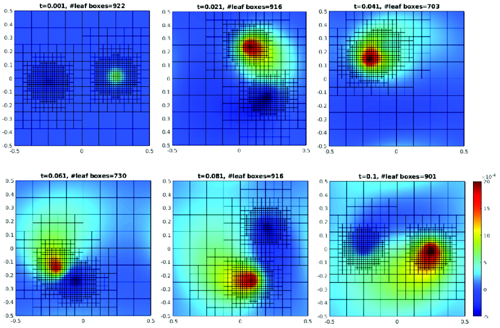
$\|\ell\|_{max}$	73	256	952
$N_{T}$	25	200	1000
error	$1.5\cdot 10^{-2}$	$4.0\cdot 10^{-5}$	$8.3\cdot 10^{-8}$

Note that the order of accuracy in space and time is sufficiently high that the error is dominated by the choice of $\epsilon^{*}$ , which determines the accuracy of the representation of the forcing function.

6.2 A semilinear heat equation in a periodic box

For our second example, we again impose periodic boundary conditions on the box $B=[-0.5,0.5]^{2}$ , but consider a semilinear heat equation using the implicit Adams-Moulton integrator. Recall that, in the integral equation formulation, this requires only the solution of scalar nonlinear equations. We solve

	$\displaystyle u_{t}({\bf x},t)$	$\displaystyle=\Delta u({\bf x},t)+F(u,{\bf x},t),\qquad{\bf x}\in B$		(113)
	$\displaystyle u({\bf x},0)$	$\displaystyle=f({\bf x},0),\qquad{\bf x}\in B,$		(113)

where $F(u,{\bf x},t)=u^{2}({\bf x},t)-f^{2}({\bf x},t)+f_{t}({\bf x},t)-\Delta f({\bf x},t)$ , with exact solution

f({\bf x},t)=\sin(2\pi x_{1})\cos(2\pi x_{2})e^{-t}+\cos(2\pi x_{1})\sin(2\pi x_{2})e^{-3t}.

(114)

Table 3 shows the relative $L^{2}$ errors of the numerical solution with respect to the exact solution at $T=0.2$ for various time steps and orders of accuracy. Table 4 then lists the ratios of successive errors, which are approaching the theoretical value $2^{p}$ for the $p$ th order scheme as ${\Delta t}$ decreases.

Table 3: The relative

L^{2}

error of the Adams-Moulton scheme for solving (113). The column heading

A_{p}

indicates the use of the

p

th order Adams-Moulton scheme.

${N_{T}}$	${{\Delta t}}$	${A_{2}}$	${A_{3}}$	${A_{4}}$	${A_{5}}$	${A_{6}}$
10	${1}/{50}$	$2.3\cdot 10^{-1}$	$1.1\cdot 10^{-1}$	$6.1\cdot 10^{-2}$	$3.8\cdot 10^{-2}$	$2.6\cdot 10^{-2}$
20	${1}/{100}$	$5.9\cdot 10^{-2}$	$1.7\cdot 10^{-2}$	$6.3\cdot 10^{-3}$	$2.6\cdot 10^{-3}$	$1.2\cdot 10^{-3}$
40	${1}/{200}$	$1.5\cdot 10^{-2}$	$2.57\cdot 10^{-3}$	$5.3\cdot 10^{-4}$	$1.3\cdot 10^{-4}$	$3.5\cdot 10^{-5}$
80	${1}/{400}$	$3.7\cdot 10^{-3}$	$3.4\cdot 10^{-4}$	$3.8\cdot 10^{-5}$	$4.9\cdot 10^{-6}$	$8.0\cdot 10^{-7}$
160	${1}/{800}$	$9.3\cdot 10^{-4}$	$4.4\cdot 10^{-5}$	$2.6\cdot 10^{-6}$	$1.7\cdot 10^{-7}$	$1.7\cdot 10^{-8}$
320	${1}/{1600}$	$2.3\cdot 10^{-4}$	$5.6\cdot 10^{-6}$	$1.7\cdot 10^{-7}$	$5.7\cdot 10^{-9}$	$2.6\cdot 10^{-10}$

Table 4: Ratios of succesive errors in Table 3.

${A_{2}}$	${A_{3}}$	${A_{4}}$	${A_{5}}$	${A_{6}}$
$3.94$	$6.21$	$9.62$	$14.79$	$22.15$
$3.98$	$6.97$	$12.04$	$20.67$	$34.09$
$4.00$	$7.45$	$13.78$	$25.39$	$43.59$
$4.00$	$7.71$	$14.82$	$28.41$	$48.06$
$4.00$	$7.85$	$15.40$	$30.54$	$63.63$

6.3 The Fujita Model

We now consider a classical reaction-diffusion process described by the equation

u_{t}=\Delta u+u^{p}.

(115)

When $p>1$ , it has been shown in [20] that the solution may blow up in finite time for the pure initial problem. For zero Dirichlet boundary conditions, with intial data given by a Gaussian, the solution will blow up in in finite time if the initial data is large (see, for example, [77] and the references therein). Here, we study the behavior of the solution with periodic boundary conditions. We choose $p=2$ and the initial data as a periodized Gaussian

u_{0}({\bf x})=5\sum_{{\bf j}\in{\bf Z}^{2}}e^{-\frac{\|{\bf x}-{\bf j}\|^{2}}{0.1}},\qquad{\bf x}\in B.

(116)

As above, we truncate the infinite lattice in the preceding expression at ( $|{\bf j}|\leq 4$ ), which is sufficient for full double precision accuracy. We use the 4th order Adams-Moulton scheme as the solver and terminate the simulation when the maximum of the solution is more than 10 times the maximum value of the initial data. The precision flag for the FGT is set to be $10^{-7}$ . We run the simulation twice, with ${\Delta t}=2\times 10^{-3}$ and ${\Delta t}=10^{-3}$ . The comparison of these two numerical solutions suggests that we have at least two digits of accuracy. Figure 7 shows snapshots of the solution at various times.

Figure 8 shows the evolution of the maximum value of the solution $u_{\rm max}(t)=\max_{{\bf x}\in B}u({\bf x},t)$ . We observe that the solution decays initially as the diffusion effect dominates the reaction component. At about $t_{c}\approx 0.099$ , the solution flattens out to being nearly a constant $u_{c}\approx 1.91$ . After that, the solution evolves as nearly constant on the whole spatial domain and follows the solution to the ODE $u_{t}=u^{2}$ , given by the formula

\frac{1}{1/u_{c}-(t-t_{c})}.

This model fits the data in Figure 8 for $t>t_{c}$ extremely well. We conjecture that, for periodic boundary conditions, the solution will blow up in finite time if the initial data is a periodized Gaussian, regardless of its magnitude. This is in stark contrast to the case of zero Dirichlet conditions. It is, perhaps, to be expected, since Dirichlet boundary conditions can be interpreted as tiling the plane with reflected Gaussians of alternating sign, while periodic conditions tile the plane with images of the same sign. We leave a rigorous analysis to the interested reader.

Figure 8: Evolution of

u_{\rm max}(t)

6.4 Heat equation in static, multiply-connected domain

To illustrate the geometric flexibility and speed of our layer potential evlauation code, in our last example we solve the heat equation in a periodic box containing 73 closed curves, on which we impose the initial condition, ${\bf u}({\bf x},0)=\sin(2\pi x_{1})\cos(2\pi x_{2})$ , and the boundary condition

{\bf u}({\bf x},t)=\sin(2\pi x_{1})\cos(2\pi x_{2})e^{-8\pi^{2}t},

where ${\bf x}\in\Gamma$ (see Fig. 9.)

The boundary is discretized by piecewise $16$ th order Legendre polynomials, with 74752 boundary points in total. A level-restricted quadtree is created so that the initial condition is resolved to precision $\epsilon=10^{-9}$ and that each leaf box contains no more than $16$ points. The tree has $9$ levels and $17647$ leaf nodes with an $8\times 8$ tensor product Chebyshev grid in each. This leads to around $10^{6}$ grid points in the unit box and $\Delta x\approx 10^{-4}$ (side length of the smallest leaf node).

We solve this boundary value problem with a second-order predictor-corrector method in time, with $8$ quadrature nodes in time each for the evaluation of $D_{NH}$ and $D_{L}$ . The step size $\Delta t=10^{-8}$ is chosen so that $\Delta t\approx\Delta x^{2}$ . The total CPU time consumed in one time step is $17.6$ seconds: $0.6$ seconds for $D_{FH}$ , $10.8$ seconds for $D_{NH}$ , and $6.27$ seconds for $D_{L}$ . The relative $L^{2}$ error at $T=1000\Delta t$ is $2.7\cdot 10^{-6}$ .

7 Conclusions

We have presented a collection of tools for the solution of diffusion problems in interior, exterior or periodic domains based on initial, volume and layer heat potentials. In the linear setting, these tools permit the creation of stable, explicit, fully automatic, high-order, space-time adaptive methods for complicated, moving geometries. In the semi-linear setting, a fully implicit formulation needed to handle stiff forcing terms requires only the solution of uncoupled scalar nonlinear equations.

The principal numerical algorithm used here is the fast Gauss transform, which we have shown can be used to develop “optimal complexity” algorithms for all types of heat potentials. Since there are a number of other fast algorithms available, future work will involve determining which is most suitable for implementation in three dimensions and for high-performance computing platforms. Open problems include the design of efficient quadratures for discontinuous forcing functions (without excessive adaptivity at the discontinuities), the design of high order representations for moving geometries involving free boundaries, and the design of robust integral representations for systems of diffusion equations.

In the present work, we have assumed that the diffusion coefficient itself is constant. We are currently working on integral equation methods that can handle piecewise-constant and piecewise-smooth diffusion coefficients, and in incorporating the solvers presented here into codes for applications including reaction-diffusion equations, crystal growth, diffusion tensor magnetic resonance imaging, and viscous fluid dynamics. Code libraries for the schemes presented here are being prepared for open source release.

Acknowledgements

We would like to thank Travis Askham, Alex Barnett, and Manas Rachh for many helpful discussions.

References

[1] B. K. Alpert. Hybrid Gauss-trapezoidal quadrature rules. SIAM J. Sci. Comput., 20:1551–1584, 1999.
[2] D. N. Arnold and P. Noon. Coercivity of the single layer heat potential. J. Comput. Math, 7:100–104, 1989.
[3] Travis Askham and Antoine J. Cerfon. An adaptive fast multipole accelerated poisson solver for complex geometries. J. Comput. Phys., 344:1–22, 2017.
[4] Alex Barnett and J. Magland. Non-uniform fast Fourier transform library of types $1$ , $2$ , $3$ in dimensions $1$ , $2$ , $3$ . https://github.com/ahbarnett/finufft, 2018.
[5] Alex H Barnett, Charles L Epstein, Leslie Greengard, Shidong Jiang, and Jun Wang. Explicit unconditionally stable methods for the heat equation via potential theory. arXiv preprint arXiv:1902.08690, 2019.
[6] J. P. Boyd. Chebyshev and Fourier Spectral Methods. Dover, New York, 2001.
[7] K. Brattkus and D. I. Meiron. Numerical simulations of unsteady crystal growth. SIAM J. Appl. Math., 52(5):1303–1320, 1992.
[8] S. Chandrasekaran, P. Dewilde, M. Gu, W. Lyons, and T. Pals. A fast solver for HSS representations via sparse matrices. SIAM J. Matrix Anal. Appl., 29:67–81, 2006.
[9] H. Cheng, L. Greengard, and V. Rokhlin. A fast adaptive multipole algorithm in three dimensions. J. Comput. Phys., 155(2):468–498, 1999.
[10] H. Cheng, J. Huang, and T. J. Leiterman. An adaptive fast solver for the modified Helmholtz equation in two dimensions. J. Comput. Phys., 211:616–637, 2006.
[11] M. Costabel. Time-dependent problems with the boundary integral equation. In E. Stein, R. de Borst, and T. J. R. Hughes, editors, Encyclopedia of Computational Mechanics, pages 703–721. John Wiley & Sons, New York, 2004.
[12] P. J. Davis and P. Rabinowitz. Methods of numerical integration. Academic Press, San Diego, 1984.
[13] Mark de Berg, Otfried Cheong, Markvan Kreveld, and Mark Overmars. Computational Geometry: Algorithms and Applications. Springer, Berlin, 2008.
[14] A. Dutt and V. Rokhlin. Fast Fourier transforms for nonequispaced data. SIMA J. Sci. Comput., 14:1368–1393, 1993.
[15] A. Dutt and V. Rokhlin. Fast Fourier transforms for nonequispaced data. II. Appl. Comput. Harmon. Anal., 2:85–100, 1995.
[16] James F. Epperson. On the use of Green’s functions for approximating nonlinear parabolic pdes. Applied Math. Letters, 2:293–296, 1989.
[17] F. Ethridge and L. Greengard. A New Fast-Multipole Accelerated Poisson Solver in Two Dimensions. SIAM Journal on Scientific Computing, 23:741–760, 2001.
[18] W. Fong and E. Darve. The black-box fast multipole method. J. Comput. Phys., 228(23):8712–8725, 2009.
[19] A. Friedman. Partial Differential Equations of Parabolic Type. Prentice-Hall, Englewood Cliffs, New Jersey, 1964.
[20] Hiroshi Fujita. On the blowing up of solutions of the Cauchy problem for $u_{t}=\Delta u+u^{1+\alpha}$ . J. Fac. Sci. Univ. Tokyo Sect. I, 13:109–124 (1966), 1966.
[21] A. Gillman, P. M. Young, and P.-G. Martinsson. A direct solver with $O(N)$ complexity for integral equations on one-dimensional domains. Front. Math. China, 7(2):217–247, 2012.
[22] Z. Gimbutas and V. Rokhlin. A generalized fast multipole method for nonoscillatory kernels. SIAM J. Sci. Comput., 24:796–817, 2003.
[23] L. Greengard and J.Y. Lee. Accelerating the nonuniform fast Fourier transform. SIAM Rev., 46:443–454, 2004.
[24] L. Greengard and P. Lin. Spectral approximation of the free-space heat kernel. Appl. Comput. Harmon. Anal., 9:83–97, 2000.
[25] L. Greengard and V. Rokhlin. A fast algorithm for particle simulations. J. Comp. Phys., 73(2):325–348, 1987.
[26] L. Greengard and V. Rokhlin. A new version of the fast multipole method for the Laplace equation in three dimensions. Acta. Numer., 6:229–270, 1997.
[27] L. Greengard and J. Strain. A fast algorithm for the evaluation of heat potentials. Comm. on Pure and Appl. Math, 43:949–963, 1990.
[28] L. Greengard and J. Strain. The fast Gauss transform. SIAM J. Sci. Statist. Comput., 12:79–94, 1991.
[29] L. Greengard and X. Sun. A new version of the fast Gauss transform. Documenta Mathematica, III pp, pages 575–584, 1998.
[30] R. B. Guenther and J. W. Lee. Partial differential equations of mathematical physics and integral equations. Prentice Hall, Inglewood Cliffs, New Jersey, 1988.
[31] Bertil Gustafsson, Heinz-Otto Kreiss, and Joseph Oliger. Time-dependent problems and difference methods. Pure and Applied Mathematics. John Wiley & Sons, Hoboken, NJ, 2nd edition, 2013.
[32] Bertil Gustafsson, Heinz-Otto Kreiss, and Arne Sundström. Stability theory of difference approximations for mixed initial boundary value problems. II. Math. Comp., 26:649–686, 1972.
[33] Wolfgang Hackbusch. Hierarchical Matrices: Algorithms and Analysis. Springer, 2015.
[34] E. Hansen and A. Ostermann. Exponential splitting for unbounded operators. Math. Comp., 78:1485–1496, 2009.
[35] Helmut Harbrecht and Johannes Tausch. An efficient numerical method for a shape-identification problem arising from the heat equation. Inverse Problems, 27(6):065013, 18, 2011.
[36] Helmut Harbrecht and Johannes Tausch. On shape optimization with parabolic state equation. In Trends in PDE constrained optimization, volume 165 of Internat. Ser. Numer. Math., pages 213–229. Birkhäuser/Springer, Cham, 2014.
[37] K. L. Ho and L. Greengard. A fast direct solver for structured linear systems by recursive skeletonization. SIAM J. Sci. Comput., 34(5):A2507–A2532, 2012.
[38] Kenneth L. Ho and Lexing Ying. Hierarchical interpolative factorization for elliptic operators: differential equations. Comm. Pure Appl. Math., 69(8):1415–1451, 2016.
[39] Kenneth L. Ho and Lexing Ying. Hierarchical interpolative factorization for elliptic operators: integral equations. Comm. Pure Appl. Math., 69(7):1314–1353, 2016.
[40] Jingfang Huang, Ming-Chih Lai, and Yang Xiang. An integral equation method for epitaxial step-flow growth simulations. J. Comput. Phys., 216(2):724–743, 2006.
[41] M. T. Ibanez and H. Power. An efficient direct BEM numerical scheme for phase change problems using Fourier series. Computer Methods in Applied Mechanics and Engineering, 191:2371–2402, 2002.
[42] T. Jahnke and C. Lubich. Error bounds for exponential operator splittings. BIT, 40:735–744, 2000.
[43] S. Jiang, L. Greengard, and S. Wang. Efficient separated sum-of-exponentials approximations for the heat kernels and their applications. Adv. Comput. Math., 41(3):529–551, 2015.
[44] H. Langston, L. Greengard, and D. Zorin. A free-space adaptive FMM-based pde solver in three dimensions. Comm. Appl. Math. Comp. Sci., 6:79–122, 2011.
[45] Dongryeol Lee, Alexander Gray, and Andrew Moore. Dual-tree fast gauss transforms. Advances in Neural Information Processing Systems, 18:747–754, 2006.
[46] J. Y. Lee, L. Greengard, and Z. Gimbutas. NUFFT Version 1.3.2 Software Release. http://www.cims.nyu.edu/cmcl/nufft/nufft.html, 2009.
[47] June-Yub Lee and Leslie Greengard. A direct adaptive Poisson solver of arbitrary order accuracy. Journal of computational physics, 125:415–424, 1996.
[48] J.Y. Lee and L. Greengard. The type 3 nonuniform FFT and its applications. J. Comput. Phys., 206:1–5, 2005.
[49] J. R. Li and L. Greengard. High order accurate methods for the evaluation of layer heat potentials. SIAM J. Sci. Comput., 31:3847–3860, 2009.
[50] Jing-Rebecca Li and Leslie Greengard. On the numerical solution of the heat equation. I. Fast solvers in free space. J. Comput. Phys., 226(2):1891–1901, 2007.
[51] Yingzhou Li and Lexing Ying. Distributed-memory hierarchical interpolative factorization. Res. Math. Sci., 4:Paper No. 12, 23, 2017.
[52] P. Lin. On the Numerical Solution of the Heat Equation in Unbounded Domains. PhD thesis, Courant Institute of Mathematical Sciences, New York University, New York, 1993.
[53] D. Malhotra and G. Biros. PVFMM: a parallel kernel independent FMM for particle and volume potentials. Commun. Comput. Phys., 18(3):808–830, 2015.
[54] D. Malhotra and G. Biros. Algorithm 967: A distributed-memory fast multipole method for volume potentials. ACM Trans. Math. Softw., 43:1–17, 2016.
[55] Robert I. McLachlan and G. Reinout W. Quispel. Splitting methods. Acta Numerica, 11:341–434, 2002.
[56] Michael Messner, Martin Schanz, and Johannes Tausch. A fast Galerkin method for parabolic space-time boundary integral equations. J. Comput. Phys., 258:15–30, 2014.
[57] Michael Messner, Martin Schanz, and Johannes Tausch. An efficient Galerkin boundary element method for the transient heat equation. SIAM J. Sci. Comput., 37(3):A1554–A1576, 2015.
[58] Victor Minden, Kenneth L. Ho, Anil Damle, and Lexing Ying. A recursive skeletonization factorization based on strong admissibility. Multiscale Model. Simul., 15(2):768–796, 2017.
[59] A. Murua and J. Sanz-Serna. Order conditions for numerical integrators obtained by composing simpler integrators. Phil. Trans. R. Soc. Lond. A, 357:1079–1100, 1999.
[60] Stanley Osher. Stability of difference approximations of dissipative type for mixed initial-boundary value problems. I. Math. Comp., 23:335–340, 1969.
[61] W. Pogorzelski. Integral equations and their applications. Pergamon Press, Oxford, 1966.
[62] D. Potts, G. Steidl, and M. Tasche. Fast fourier transforms for nonequispaced data: A tutorial. Modern Sampling Theory Mathematics and Applications, pages 249–274, 2001.
[63] R. S. Sampath, H. Sundar, and S. Veerapaneni. Parallel fast Gauss transform. in SC Proceedings of the ACM/IEEE International Conference for High Performance Computing, Networking, Storage and Analysis, New Orleans, LA, 10:1–10, 2010.
[64] James A. Sethian and John Strain. Crystal growth and dendritic solidification. J. Comput. Phys., 98:231–253, 1992.
[65] Marina Spivak, Shravan K. Veerapaneni, and Leslie Greengard. The fast generalized Gauss transform. SIAM J. Sci. Comput., 32(5):3092–3107, 2010.
[66] J. Strain. The fast Gauss transform with variable scales. SIAM J. Sci. Stat. Comput., 12:1131–1139, 1991.
[67] J. Strain. Fast adaptive methods for the free-space heat equation. SIAM J. Sci. Comput., 15:185–206, 1994.
[68] Gilbert Strang. On the construction and comparison of difference schemes. SIAM J. Numer. Anal., 5:506–517, 1968.
[69] John C. Strikwerda. Finite difference schemes and partial differential equations. SIAM, Philadelphia, PA, 2004.
[70] J. Tausch and A. Weckiewicz. Multidimensional fast Gauss transforms by Chebyshev expansions. SIAM J. Sci. Comput., 31:3547–3565, 2009.
[71] Johannes Tausch. A fast method for solving the heat equation by layer potentials. J. Comput. Phys., 224(2):956–969, 2007.
[72] Johannes Tausch. Nyström discretization of parabolic boundary integral equations. Appl. Numer. Math., 59(11):2843–2856, 2009.
[73] Johannes Tausch. Fast Nyström methods for parabolic boundary integral equations. In Fast boundary element methods in engineering and industrial applications, volume 63 of Lect. Notes Appl. Comput. Mech., pages 185–219. Springer, Heidelberg, 2012.
[74] L. Trefethen. Numerical computation of the Schwarz-Christoffel transformation. SIAM J. Sci. Stat. Comput., 1:82–102, 1980.
[75] Lloyd N. Trefethen. Group velocity interpretation of the stability theory of Gustafsson, Kreiss, and Sundström. J. Comput. Phys., 49(2):199–217, 1983.
[76] R. Tyson, L. G. Stern, and R. J. LeVeque. Fractional step methods applied to a chemotaxis model. J. Math. Biol., 41:455–475, 2000.
[77] Juan Luis Vázquez. The Mathematical Theories of Diffusion: Nonlinear and Fractional Diffusion, pages 205–278. Springer International Publishing, Cham, 2017.
[78] S. K. Veerapaneni and G. Biros. A high-order solver for the heat equation in 1d domains with moving boundaries. SIAM J. Sci. Comput., 29:2581–2606, 2007.
[79] S. K. Veerapaneni and G. Biros. The Chebyshev fast Gauss and nonuniform fast Fourier transforms and their application to the evaluation of distributed heat potentials. J. Comput. Phys., 227:7768–7790, 2008.
[80] X. Wan and G. Karniadakis. A sharp error estimate for the fast Gauss transform. Journal of Computational Physics, 219:7–12, 2006.
[81] J. Wang. Integral equation methods for the heat equation in moving geometry. PhD thesis, Courant Institute of Mathematical Sciences, New York University, New York, September 2017.
[82] J. Wang and L. Greengard. Hybrid asymptotic/numerical methods for the evaluation of layer heat potentials in two dimensions. Adv. Comput. Math., 45(2):847–867, 2019.
[83] Jun Wang and Leslie Greengard. An adaptive fast Gauss transform in two dimensions. SIAM J. Sci. Comput., 40(3):A1274–A1300, 2018.
[84] S. Wang. Efficient High-Order Integral Equation Methods for the Heat Equation. PhD thesis, Department of Mathematical Sciences, New Jersey Institute of Technology, Newark, New Jersey, August 2016.
[85] Shaobo Wang, Shidong Jiang, and Jing Wang. Fast high-order integral equation methods for solving boundary value problems of two dimensional heat equation in complex geometry. Journal of Scientific Computing, 79(2):787–808, 2019.
[86] L. Ying, G. Biros, and D. Zorin. A kernel-independent adaptive fast multipole algorithm in two and three dimensions. J. Comput. Phys., 196:591–626, 2004.
[87] Bo Zhang, Jingfang Huang, Nikos P. Pitsianis, and Xiaobai Sun. A Fourier-series-based kernel-independent fast multipole method. J. Comput. Phys., 230(15):5807–5821, 2011.