Cosmic Microwave Background Anisotropy numerical solution (CMBAns) I: An introduction to calculation
Abstract
Cosmological Boltzmann codes are often used by researchers for calculating the CMB angular power spectra from different theoretical models, for cosmological parameter estimation, etc. Therefore, the accuracy of a Boltzmann code is of utmost importance. Different Markov Chain Monte Carlo based parameter estimation algorithms typically require iterations of Boltzmann code. This makes the time complexity of such codes another critical factor. In the last two decades, several Boltzmann packages, such as CMBFAST, CAMB, CMBEasy, CLASS etc., have been developed. In this paper, we present a new cosmological Boltzmann code, CMBAns, that can be used for accurate calculation of the CMB power spectrum and BipoSH coefficients. At present, CMBAns is developed for a flat background matrix. It is mostly written in the C language. However, we borrowed the concept of class from C++. This gives researchers the flexibility to develop their own independent package based on CMBAns, without an in-depth understanding of the source code. We also develop multiple stand-alone facilities which can be directly compiled and run on a given parameter set. In this paper, we discuss all the mathematical formulation, approximation schemes, integration methods etc., that are used in CMBAns. The package will be made available through github for public use in the near future.
1 Introduction
Since the discovery of the Cosmic Microwave Background (CMB) by Penzias and Wilson, the CMB has become an invaluable probe for understanding the physics in the early universe. Several cosmological theories, proposed in the past, failed to explain the origin of CMB. Hence, they were rejected as feasible cosmological theories. Others like Big Bang cosmology, with some assumptions, provide a more complete explanation of the origin of CMB radiation. These models later, after several theoretical modifications, were accepted as the standard cosmological models. Hence, the discovery of CMB marked the path for the birth of standard cosmology.
The precision of the CMB observation has improved over the years. In the past decade, several ground-based and space-based experiments like WMAP, Planck, BICEP, ACT etc. have measured the CMB temperature to an exquisite precision. Future experiments like SPT-3G and Simons Array will provide even better measurements of CMB temperature and polarization (Abazajian et al. 2016). To analyze this influx of data and to test different cosmological models, we also need more accurate Boltzmann codes.
The theory of cosmological perturbations for standard model cosmology was first developed by Lifshitz (Lifshitz 1946) and later was reviewed by many others (Lifshitz and Khalatnikov 1963). The subsequent research works are summarized in review articles (Kodama and Sasaki 1984; Mukhanov et al. 1992), in books and in theses (Weinberg 2008; Tassev 2011). Lifshitz used the synchronous gauge for formulating the linear perturbation theory. Later, Bardeen and others developed the perturbation theory in the conformal gauge due to some complications with the synchronous gauge, such as the appearance of the coordinate singularity (Kodama and Sasaki 1984; Bardeen 1980) etc. The conformal gauge is more frequently used for analytical calculations of the cosmological perturbation equations. However, the synchronous gauges are preferred for the numerical calculations due to the stability issues (Montani et al. 2011; Hu 2004).
The Boltzmann codes have been in use in cosmology for a long time to calculate the CMB angular power spectrum. The first of such code provided in the public domain was COSMICS (Ma and Bertschinger 1995), written by Ma and Bertschinger. Later, Seljac and Zaldarriaga developed CMBFAST (Seljak and Zaldarriaga 1996; Zaldarriaga et al. 2001), in which the line-of-sight integration method was used to make the power spectrum calculation faster. Since then, several packages utilizing Boltzmann codes, such as CAMB (Lewis), CMBEasy (Doran 2005), CLASS (Lesgourgues 2011a; Blas et al. 2011; Lesgourgues 2011b; Lesgourgues and Tram 2011), PyCosmo (Refregier et al. 2018) etc., have come into existence. In this paper, we describe a new Boltzmann code, called CMBAns (Cosmic Microwave Background Anisotropy numerical solution). The package is based on CMBFAST and was initially developed in 2010 for a variety of CMB studies (Das 2010; Das et al. 2013; Das and Souradeep 2014a).
There are three principal motivations behind developing CMBAns. First of all, in future CMB missions, the precision of the CMB measurements will improve drastically. Hence, the Boltzmann packages should be able to calculate the CMB power spectrum very accurately up to high multipoles. Secondly, different Markov Chain Monte Carlo (MCMC) packages, such as CosmoMC (Lewis and Bridle 2002; Lewis 2013), SCoPE (Das and Souradeep 2014b), AnalyzeThis (Doran and Mueller 2004), etc, which are often used to estimate the cosmological parameters, typically require - evaluations of Boltzmann codes. Therefore, the Boltzmann code should be able to calculate the CMB power spectrum fast and efficiently. Thirdly, most of the present Boltzmann codes follow a monolithic architecture design and are not modular. Therefore, it is difficult to add any new feature in the package and the functions cannot be used independently. Users cannot write their own packages and use existing functions without an extensive knowledge of the entire source code. To overcome this limitation, CLASS code introduced a modular architecture. CMBAns is also written in a modular format. It consists of several stand-alone codes, as well as some user-defined functions that users can use to write their codes.
CMBAns solves the linear Boltzmann equations for different constituents of the universe and thereafter uses the line-of-sight integration approach to calculate the source terms and the brightness fluctuations. These are then convolved with the primordial power spectrum to get the CMB angular power spectrum. CMBAns can calculate the cosmological power spectrum for different dark energy models (both perturbed and unperturbed), two-field inflation model, etc. CMBAns also comes with a MATLAB GUI, where the Hubble parameter of the universe can be visually modified as a function of redshift. CMBAns translates the modified Hubble parameter into the dark energy equation of state (EOS) and then computes the CMB power spectrum for that particular model (Das and Souradeep 2014a). Apart from these, CMBAns can also calculate the isotropy violation signals by calculating the BipoSH coefficients along with the angular power spectrum in presence of anisotropic inflation (Das et al. 2014).
This is the first paper, in a series of papers about to come on CMBAns. In this paper, we describe all the mathematical equations and the discretization techniques that are used in CMBAns. We also briefly describe the cosmological perturbation theory in the synchronous gauge and discuss the equations and approximation schemes used in developing CMBAns. The paper is divided into eight sections. In the second section, we describe the conformal time calculations between any two eras in the universe. In the third section, we describe different recombination processes, calculating the baryon temperature, sound speed etc. The fourth section discusses CMB perturbation calculations and different approximation schemes used in CMBAns, and how they affect the power spectrum calculations. Different scalar and tensor initial conditions are discussed in the fifth section. The sixth and seventh sections are for line-of-sight integration and calculating the power spectra and the BipoSH coefficients for anisotropic inflation. The numerical techniques, time and wave number space grid etc. are discussed in the eighth section. The final section is for discussion and conclusion.
2 Conformal time calculation
In cosmology, the redshift is often used for measuring time. However, for numerical calculation of the perturbation equations, line-of-sight integration, etc. the conformal time plays an important role. It is straight-forward to calculate the conformal time under the assumption of a matter-dominated or dark energy-dominated universe. However, in the presence of all the components of the universe, the calculations can be complicated and an analytical solution may not exist.
In this paper, we denote the conformal time as . The Hubble parameter is defined as
| (2.1) |
where is the scale factor. From the FLRW equation, we can write the Hubble parameter as
| (2.2) |
The above two equations give
| (2.3) |
where , , and are the density parameters for present-day matter (which include both cold dark matter and baryonic mater), photon, and massless neutrinos respectively. The density parameter of massive neutrinos and dark energy at a scale factor are and , respectively. The density parameters are defined as the ratios of the respective densities over the critical density:
where, the critical density is given by . The densities of matter and radiation at any era are scaled as , , respectively with their densities at the present era. For calculating the density of the massive neutrinos, we need to use the Fermi-Dirac statistics. For dark energy model, the density of the dark energy will be constant. However, for any other dark energy model, we need to calculate the density variation from its equation of state (eos).
2.1 Matter density
The first term in Eq. 2.3 can be calculated by evaluating . As the CDM and baryon density parameters, and are the input parameters, we can calculate . is also an input parameter, but its unit is km/sec/Mpc. In CMBAns, we use Mpc as the unit for both the spatial and temporal dimensions. In order to convert the Hubble parameter in , we multiply with .
2.2 Radiation density for photons
The radiation density consists of two components: photon density and the massless (relativistic) neutrino density . The photon number density as a function of frequency can be derived from the Planck radiation law:
| (2.4) |
where is the Boltzmann constant, is the Planck constant, and is the current CMB temperature. The photon energy density can be calculated as
| (2.5) |
where is the radiation constant. We also know that
| (2.6) |
Therefore, the second term in Eq. 2.3 can be calculated by evaluating as follows
| (2.7) |
2.3 Radiation density for massless neutrinos
Massless neutrinos follow Fermi-Dirac statistics with neutrino temperature . The distribution function is given by
| (2.8) |
We can calculate the radiation density of the massless neutrinos as
| (2.9) |
For relating the temperatures between photon and neutrinos, consider the era before neutrino and photon decoupling. In that ultra high energy regime, as photon and neutrino were coupled, the medium in which they existed had a fixed temperature. Other species in the medium were electrons (2 spin states), positrons (2 spin states), neutrinos (1 spin state for each of the three generations), and antineutrinos (1 spin states for each of the three generations). Shortly after the photon and neutrino decoupling, the temperature drops below the electron mass, and the forward reaction (annihilation) becomes strongly favored. This heats up the photons. We can assume that this entropy transfer did not affect the neutrinos because they were already completely decoupled. Using entropy conservation of the electromagnetic plasma, we can calculate the change in the photon temperature before and after annihilation. This gives (Dodelson 2003)
The neutrino density is related to the photon density by
where is the effective number of neutrinos. Theoretically, there are 3 neutrino families. However, due to non-instantaneous decoupling and QED effects etc. the effective neutrino density will be slightly higher then this value. This can be accounted for by considering . Considering a general framework for neutrino decoupling, it can be shown that for non instantaneous neutrino decoupling, . In addition, the QED effects contribute about . Assuming these two effects can be added linearly, the final value of (Dolgov et al. 1997; Dolgov et al. 1998; Mangano et al. 2001; Grohs et al. 2015; Escudero 2018; Salas and Pastor 2016).
Therefore, the third term in Eq. 2.3 can be calculated as
| (2.10) |
2.4 Radiation density for massive neutrinos
In standard model of particle physics, neutrinos are massless. However, different experiments point toward a small nonzero mass for the neutrinos. For massive neutrinos, the Fermi-Dirac distribution function contains mass term, and it is not analytically integrable. Therefore, to get the density at any given redshift, the distribution function must be integrated numerically.
Assuming that all the neutrino species have equal mass, the mass of the neutrinos is given by
| (2.11) |
where is the effective number of neutrinos. and are the massive neutrino density and number density at present time respectively. is the critical density.
The neutrino number density can be calculated by integrating the Fermi-Dirac distribution function:
| (2.12) |
For neutrinos , and we can ignore the term in the above equation. This simplifies to
| (2.13) |
where is the Riemann Zeta function and is the Gamma function. .
The density and pressure of massive neutrinos at any given redshift can be written as
| (2.14) | |||||
| (2.15) |
where and,
| (2.16) |
Here, in Eq. 2.15 the factor of 3 comes because we consider 3 spatial dimensions11 1 For an ideal gas, the pressure can be found by . is the number density of the gas molecule, is the velocity, and is the mass of each gas molecules. The factor of 3 arises because we have considered 3 special dimensions and we consider that the velocity distribution of the gas is isotropic, i.e. . Eq. 2.15 can also be derived in a similar way, where corresponds to the momentum.. Simple re-arrangements of the above equations give us the massive neutrino density and pressure in terms of massless neutrino density, as
| (2.17) | |||||
| (2.18) |
Here and are dimensionless density and pressure and are expressed as
| (2.19) | |||||
| (2.20) |


where 22 2 Note that for calculating we need the Bose-Einstein integration formula, .. In Fig. 1, we plot the dimensionless density and pressure for massive neutrinos for different density parameters, (note that , where is the the Hubble parameter in units of ) (Mangano et al. 2005). In the early universe, where the temperature is high, , the neutrinos behave like massless particles and and . However, later, where dominates, the massive neutrinos start behaving like matter particles and and , i.e. the actual density of the massive neutrinos goes as .
2.5 Contribution from dark energy
The last term in Eq. 2.3 is the contribution from the dark energy. We can use the approximation (since , , are of the order of ). For a CDM model, the equation of state for dark energy is . However, several dark energy models have been proposed over years based on a single scalar field, a mixture of multiple scalar fields, e.g. quintessence (Ratra and Peebles 1988), K-essence (Armendariz-Picon et al. 2000; Chiba et al. 2000; Armendariz-Picon et al. 2001), tachyon (Padmanabhan 2002; Bagla et al. 2003), dilatonic models (Kamenshchik et al. 2001); massive vector field (Koivisto and Mota 2008; Boehmer and Harko 2007) etc. For different dark energy models, the equation of state for dark energy may vary as a function of scale factor, i.e. . In such cases we can write the generalized form of as
| (2.21) |
CMBAns is capable of handling both the constant or a varying equation of state, , models of dark energy. Presently there is tension between the Hubble parameter measured using the Planck and using supernova data. Astronomers are trying to model the Hubble parameter as a function of redshift and modify the dark energy accordingly. In CMBAns we add modules which allow users to provide Hubble parameter as a function of redshift using Matlab-GUI input. CMBAns translate the Hubble parameters as equation of state of dark energy (Das and Souradeep 2014a) and calculate the CMB power spectrum. CMBAns also provides the primordial, late time ISW and interference term between the primordial and late time ISW along with the full power spectrum to show the effect of late time expansion history of the universe on the CMB power spectrum.
Fig. 2 shows the variation of as a function of scale factor for different values of and for standard CDM model. The conformal time between two given redshifts can be calculated by numerically integrating Eq. 2.3. For various dark energy models the shape of the CMB power spectra changes. In Fig. 3 and Fig. 4 we demonstrate the special feature of CMBAns where we can select the deviation in Hubble parameter from the standard CDM Hubble parameter () as a function of redshift using a Matlab GUI input. The deviation that we have selected for this illustration is shown in Fig. 3. We try to keep the distance to the last scattering surface to be constant. The temperature power spectrum that we get for this particular deviation deviation of Hubble parameter is shown in Fig. 4. An interesting fact for such kind of deviation is that the ISW part provides a very small contribution, sometimes even negative contribution to the . For this particular illustration, we have not consider any re-ionization. This is because purpose of the illustration is to show the particular form of the late time ISW effect which is not an well known phenomenon. As the polarization part don’t have any ISW contribution, there will be no such effect on the polarization power spectra (Das and Souradeep 2014a). Without a GUI input, exploring such model would have been immensely difficult.
3 Recombination and Reionization
For calculating the baryon sound speed, optical depth, and visibility function, we need to calculate the recombination and the reionization process very accurately. CMBAns provides functions for calculating the recombination using the Saha equation, Peebles equation, recfast or CosmoRec method.
3.1 Saha Equation
Saha equation provides a very rough estimate of the recombination epoch. It assumes the recombination reaction is fast enough that it proceeds near thermal equilibrium, i.e. it ignores the expansion of the universe. According to the Saha equation,
| (3.1) |
where is the hydrogen ionization fraction. is the number density of the hydrogen atoms, i.e. , where and are number density of neutral hydrogen and ionized hydrogen, respectively. is the ionization potential of the hydrogen atom. is the baryon temperature.
The hydrogen number density can be calculated as
| (3.2) |
3.2 Peebles’ Recombination
Peebles’ equation provides a very accurate estimate of the recombination history of hydrogen. The calculations are done using effective three-level atom calculations. Peebles’ formalism is based on the assumptions that
- •
Direct recombinations to the ground state of hydrogen are very inefficient: each such event leads to a photon with energy greater than , which almost immediately re-ionizes a neighboring hydrogen atom. Electrons therefore only efficiently recombine to the excited states of hydrogen, from which they cascade very quickly down to the first excited state, with principal quantum number .
- •
From the first excited state, electrons can reach the ground state through two pathways:
- 1.
Decay from the 2p state by emitting a Lyman- photon. This photon will almost always be reabsorbed by another hydrogen atom in its ground state. However, cosmological redshifting systematically decreases the photon frequency, and hence there is a small chance that it escapes reabsorption if it gets redshifted far enough from the Lyman- line resonant frequency before encountering another hydrogen atom.
- 2.
Decay from the to state, which is only possible using an electron double transition. The rate of this transition is very slow, . It is however competitive with the slow rate of Lyman- escape in producing ground-state hydrogen.
- 1.
- •
Atoms in the first excited state may also be re-ionized by the ambient CMB photons before they reach the ground state, as if the recombination to the excited state did not happen in the first place. To account for this possibility, Peebles defines the factor as the probability that an atom in the first excited state reaches the ground state through either of the two pathways described above before being photo-ionized.
Accounting for these processes, the recombination history is then described by the differential effect (Peebles 1968)
| (3.3) |
where
| (3.4) |
The recombination rate to excited states (Ma and Bertschinger 1995) is taken as
| (3.5) |
This expression for provides a good approximation at low temperature. At high temperature this expression underestimates , but the amount is negligible. For , we set .
| (3.6) |
where
| (3.7) |
, is the wavelength for Lyman- emission. Over-dot represents the derivative with respect to the conformal time. is the rate of hydrogen double transition from to . .
| (3.8) | |||||
Similarly, can be calculated using
where . Here, is in unit, and has unites of unit. The numerical values are converted to match these units.
Helium Recombination
For calculating the He recombination, we use the Saha Equation (Ma and Bertschinger 1995).
| (3.9) |
where , and . The helium ionization fractions and , where is the total number density of helium nuclei. is the free electron number density. and . and are the first and second ionization temperature of He.
3.3 Recfast, CosmoRec
Peebles’ three-level atom model accounts for the most important physical processes. However, these approximations may lead to errors on the predicted recombination history at a level as high as . This can also alter the temperature and polarization power spectra up to at high multipoles. Several research groups have revisited the details and proposed different models like recfast33 3 https://www.cfa.harvard.edu/~sasselov/rec/(Seager et al. 1999; Seager et al. 1999), CosmoRec44 4 http://www.jb.man.ac.uk/~jchluba/Science/CosmoRec/Welcome.html(Chluba and Thomas 2010; Ali-Haïmoud and Hirata 2010a; Chluba et al. 2010; Switzer and Hirata 2008; Grin and Hirata 2010; Rubiño-Martín et al. 2010), HyRec55 5 https://cosmo.nyu.edu/yacine/hyrec/hyrec.html(Ali-Haïmoud and Hirata 2010b) etc. These packages can calculate the recombination history up to accuracy. We use the available CosmoRec code in CMBAns as a default case. However, users can choose to use Saha, Peebles or recfast routine which are also available in CMBAns. The other packages can also be easily added in the CMBAns or run separately. In the later case the ionization fraction, and baryon temperature can be stored in a file as a function of scale factor and pass it to CMBAns.
In Fig. 5, we show the ionization fraction from different recombination methods. We use a smooth reionization, where we join an ionization fraction before and after the reionization using a function. In Fig. 6, we show the differences between recfast, recfast++ and CosmoRec recombination. This small change in the ionization fraction can change the at high multipoles.
3.4 Calculating baryon temperature
For calculating ionization fraction during the recombination, we need the baryon temperature at each scale factor. The rate of change of the baryon temperature can be calculated as (check Appendix A)
| (3.10) |
where is the Thomson scattering cross section. is given by
| (3.11) |
is the total ionization fraction and is given by
| (3.12) |
The constant term in Eq. 3.10 is given by . We can see that the baryon temperature depends on the ionization fraction of the electrons. Therefore, we need to jointly evaluate the baryon temperature and ionization fraction. The temperature of the photons at any era is . We can consider before recombination (in the tight coupling era), and we can use it as the initial condition for solving Eq. 3.10.
3.5 Baryon sound speed, optical depth and visibility
Calculating the baryon acoustic oscillations require the speed of sound in the plasma, . If we consider the plasma as a single fluid, then the pressure, density and the temperature of the fluid will be related as . We can calculate the sound speed in the plasma as
| (3.13) | |||||
Here is the mean molecular weight of the fluid, and is the mass of a proton 66 6 For all our calculations, we consider the mass of H and H , and mass of He, He+, He, i.e. we consider that the mass of electron is negligible and the mass of proton and neutron are the same.. The mean molecular weight is calculated assuming the fluid contains free electrons, H, H+, He, He+, He++. Here one should note that a more accurate formulation of the sound speed was proposed by Lewis 2007, and are used in CAMB and CLASS. We are in process of implementing it in CMBAns.
The optical depth from the present time () to any conformal time is given by
| (3.14) |
The visibility function at any conformal time can be calculated as . In Fig. 7 we show the visibility function vs the scale factor. The visibility function is nonzero only during the recombination and reionization process. The change in the visibility function is significantly smaller during reionization, than recombination. To show both on the same plot, we multiply the reionization part by .
4 A brief overview of the cosmological perturbations
CMBAns is developed only for the flat background metric, i.e. . We can represent a completely isotropic and homogeneous expanding universe using FLRW metric, , where , and is the Minkowski metric. Since our universe is not completely homogeneous and isotropic, we need to add some perturbation to the metric. The line element in the perturbed metric is given by
| (4.1) |
Here is the perturbation in the metric. For simplicity of calculation, the metric perturbation is expanded in the spatial and temporal parts. This can be done by breaking in dimensional format as (Weinberg 2008)
| (4.2) |
where , , , , , are are the perturbation variables and
| (4.3) |
From Einstein’s equation, we get , where is the Einstein tensor, and is the stress-energy tensor. Perturbing the equations up to the first order, we get . We can use the above perturbation variables to calculate the perturbations in the Christoffel symbols. The perturbation to the Einstein’s tensor, can then be computed from the Christoffel symbols. For calculating the perturbation in , we need to know the perturbation in the pressure and density of the different components in the Universe, i.e. baryons, photons, neutrinos, dark matter, and dark energy, etc. For a perfect fluid, the stress-energy tensor is given by
| (4.4) |
Similar to the metric tensor, the perturbation in the stress-energy tensor can also be expanded into spatial and temporal parts
| (4.5) |
in which
| (4.6) |
We can match both the sides in and separate out:
- •
The terms containing , , , , , , and . These involve all the scalar quantities and are called the scalar perturbations.
- •
The terms containing , , and . These involve all the vector quantities in the spatial dimension and are called the vector perturbations. These vector modes decay and hence have a small contribution to the CMB power spectrum (Weinberg 2008).
- •
The terms involving and . These terms behave as tensor quantities in 3-spatial dimensions and are called the tensor perturbations.
4.1 Theory of scalar perturbations
We can obtain the scalar perturbation equations by separating out the terms involving the scalar perturbation variables, i.e. , , , , , , and . However, these terms are not all independent (Weinberg 2008). Also, there can be unphysical modes due to the choice of the coordinate system. These problems can be resolved by fixing a proper coordinate system, and adopting suitable conditions on the full perturbed metric and energy-momentum tensor. This process is called gauge fixing (Weinberg 2008; Ma and Bertschinger 1995). In CMBAns, we do all the calculations involving the scalar perturbation in synchronous gauge (Lifshitz 1946).
In synchronous gauge, the scalar component of the perturbed metric can be written as , where is the Kronecker delta, and is the scalar part of the metric perturbation in synchronous gauge. can be represented using only two scalar fields and , in (,) space, where
| (4.7) |
, is the unit vector along direction of vector and is its amplitude. We can relate and with the real space perturbation variables , , , . This gives , , because in synchronous gauge we take constant time hyperspace, and . The growth of these perturbation variables can be computed using the perturbed Einstein equations . The perturbation in can be calculated using the metric perturbation variables (Ma and Bertschinger 1995) as
| (4.8) | |||||
| (4.9) | |||||
| (4.10) | |||||
| (4.11) |
Here is defined as . For a fluid, this is simply the divergence of its velocity field, i.e. . The in Eq. 4.11 can be defined as , where is the anisotropic stress term, corresponding to its real space quantity shown in Eq. 4.5.
We also need to conserve the perturbation in the stress-energy tensor, i.e. . For non-relativistic perfect fluid, these conservation equations give us
| (4.12) |
where is the perturbation in the density of the fluid. is the equation of state of the fluid. Non-relativistic fluids like the CDM and baryon should obey these equations.
To calculate the stress-energy tensor for the relativistic particles, we need to use the distribution function. Photons follow the Bose-Einstein distribution, whereas the neutrinos follow the Fermi-Dirac distribution. Considering as the phase space distribution function, the stress-energy tensor is given by
| (4.13) |
is the four-momentum. . . , are the magnitude and the direction of the momentum and . It is convenient to write the distribution function as
| (4.14) |
Here in the first order perturbation in the distribution function. In synchronous gauge , and . The phase-space distribution evolves as the Boltzmann equation. If we convert everything to Fourier space ( space), then the first-order perturbations of the Boltzmann equation in the synchronous gauge can be written as
| (4.15) |
Photons and neutrinos will follow this equation. The term on the right-hand side is the collision term. Neutrinos are collisionless in our domain as they decouple long back in the radiation dominated era. However, before decoupling, the photon and baryon collisions will provide some contribution to this term.
and for photons and neutrinos can be calculated in terms of , the detail of which is discussed in Sec. 4.1.
Scalar perturbations in the metric
In the previous section, we describe the equations for the metric perturbation in terms of . However, there are the different components of the universe, i.e. CDM, baryon, photon, neutrino, DE, etc. and we need the metric perturbations in terms of perturbations of these individual components. We use the subscript , and for representing cold dark matter, baryonic matter, photon, massless neutrinos, massive neutrinos, and dark energy respectively. Following Eq. 4.8 and Eq. 4.9, the equations for the metric perturbation can be written in terms of density () and velocity perturbations () of the individual components as
| (4.16) | |||||
| (4.17) | |||||
where, over-dot () represents the derivative with respect to the conformal time and is the effective number of spin states before neutrino decoupling. For , we get . However, in presence of any other particle in the early universe, the above expression will correct for that.
Instead of the last two equations (Eq. 4.10 and Eq. 4.11), we take the conservation equations () for different components of the universe, which evolve independently except before decoupling, when the baryon and photon evolve together as a single fluid. The conservation equations for different components in terms of their density and velocity perturbations ( and ) are given below.
Conservation equation for Cold Dark Matter (CDM)
CDM can be treated as a pressure-less perfect fluid and it interacts with other particles only through gravity. Therefore, for CDM and the conservation equations, i.e Eq. 4.12, for CDM gives
| (4.18) |
As CDM does not interact with other particles, if is fixed as the initial condition then the values of will remain through the entire era. Setting also solves another purpose by removing the extra gauge mode in the synchronous gauge (Sec. 5.1). Thus the CDM equation becomes as . In Fig. 8 we show the evolution of the CDM density perturbation for different modes.
Conservation equations for massless neutrinos
According to the standard model of particle physics the neutrinos are massless. However, neutrino oscillation provides evidence for non-zero mass, but only values. Therefore, cosmologists are interested in checking the consequences of both the massive and massless neutrinos in the cosmic fluid. The perturbation equation for the massive and the massless neutrinos differ significantly.
For massless neutrinos, the density and pressure are related as , where, is the Fermi-Dirac distribution function and is the momentum in the co-moving frame. Unlike CDM, neutrinos have pressure. Therefore, solving the growth equations for neutrinos is difficult as there are several direction-dependent variables. However, for solving Eq. 4.8 – Eq. 4.11, we only need , and and these can be simplified by defining a new variable
| (4.19) |
where is the perturbation in the Fermi-Dirac distribution function i.e. , being the th order term of the Fermi-Dirac distribution function.
According to Eq. 4.15, and always appear together as , showing that only the magnitude and the angle between them are important, not the individual values of and . We can expand in terms of Legendre Polynomials as
| (4.20) |
where are the Legendre polynomials and are their coefficients.
The term is taken out to simplify the perturbation equations. For calculating the perturbation equations in terms of these variables, we can use Eq. 4.15 and Eq. 4.19 and expand them in the Legendre polynomials. The perturbation equations for massless neutrinos take the form (Ma and Bertschinger 1995)
| (4.21) | |||||
| (4.22) | |||||
| (4.23) | |||||
| (4.24) |
Here goes up to . The truncation condition can be taken as (Ma and Bertschinger 1995)
| (4.25) |
However, such a choice of truncation condition can lead to a large error in the final power spectrum calculation, due to the propagation error if the Boltzmann hierarchy is truncated after some low . For truncating the set of equations, in CMBAns we use (which the user can change to any higher value). In Fig. 9 we show the percentage errors involved in the CMB power spectrum calculation for truncating the equations at different , considering to be standard. The plots show that the error introduced due to the truncation of the neutrino equations slowly decreases with the increase in .
In Fig. 8, we show the growth of the density fluctuations in neutrino. As they don’t interact with any other species, their evolution is completely independent of others. The modes evolve as before horizon crossing. After horizon crossing, when they come in causal contact they start oscillating.
Conservation equations for massive neutrinos
For the massive neutrinos , where is the momentum in the co-moving frame and is the mass of the neutrino. Hence, unlike massless neutrinos, the expressions cannot be integrated analytically. Thus, we expand the perturbation directly in terms of Legendre polynomials as (Ma and Bertschinger 1995):
| (4.26) |
Substituting this in Eq. 4.15, the Boltzmann equations for the massive neutrinos become
| (4.27) | |||||
For truncating the series we use the condition
| (4.28) |
Here, are the functions of and . The integration over is performed numerically after calculating different massive neutrino multipoles for different . For the massive neutrinos the modes are truncated after .
Photons
Photons evolve differently before recombination, when they were tightly coupled with baryons and after recombination, when they were free streaming. The evolution of the photons can be treated in the same way as the massless neutrinos except the collision terms will be present. Thompson scattering by a density perturbation can introduce polarization in an unpolarized photon field and in a density perturbation. Therefore, along with the total intensity, we also have to consider the polarization component for the photons. The details of the polarization is discussed are Appendix B.
Defining the intensity perturbations as and the polarization as , the Boltzmann equations for photons in the synchronous gauge can be written as (Ma and Bertschinger 1995)
| (4.29) | |||||
where is the Thomson scattering cross-section, and is the free electron number density. The truncation of the Boltzmann equations is done in the same way as that of the massless neutrinos. For we can replace the and the by the following equations
| (4.30) |
The evolution of the photons is shown in Fig. 8. Before recombination, the photons are tightly coupled with the baryons, and they evolve together as a single fluid. However, after decoupling, the photons follow a similar pattern as that of the neutrinos.
For photons we choose the truncation at . The error involved due to the truncation of the photon multipole equations, i.e. is shown in Fig. 10. The errors are calculated considering to be standard. We can see that if we truncate the evaluation in low , such as or , then the error involved can be as high as . However, if we increase , the error decreases drastically. At , the error in the final is less than .
Baryons
Before recombination, the baryons and photons were tightly coupled and they evolved together as a single fluid. However, after recombination, the baryons decouple from the photons and evolve separately. The baryon density and the velocity perturbations are governed by the following equations (Ma and Bertschinger 1995)
| (4.31) |
where, and are the background density for photons and baryons respectively. is the baryon sound speed shown in Eq 3.13.
In the tight coupling era, the photon and baryon equations cannot be solved independently using the Runge-Kutta methods, as this may lead to large numerical errors. Therefore, a separate set of equations is used for solving the baryon perturbation in the tight coupling era.
Recombination and the Tight Coupling Approximation
Before recombination the opacity was very large. Hence, the photons and baryons evolve together during the tight coupling approximation. The conformal time scale for the photon baryon interaction is . In the tight coupling era, this interaction time scale is much smaller than the timescale on which the modes in the super-Hubble scale evolve, i.e. and the modes for the sub-Hubble scale i.e. . The standard numerical integration is not efficient to integrate the baryon and photon perturbation equations independently in this era. Therefore, Peebles and Yu, (Ma and Bertschinger 1995; Peebles and Yu 1970) developed a new set of equations for the baryon perturbations which is valid in the tight coupling regime i.e. where or . Instead of using the standard baryon and photon equations, the idea is to integrate a coupled form of differential equation, given by
| (4.32) |
where , and is given by the following equation
| (4.33) | |||||
For obtaining , we can use the following equation (Ma and Bertschinger 1995)
| (4.34) |
In the tight coupling limit the higher multipoles of the photon distribution, i.e. , , … and , , , … can be taken as . We also consider , which from Eq. 4.29 gives
| (4.35) |
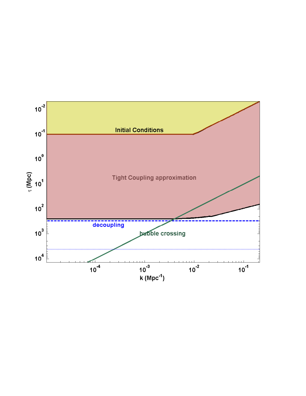
In Fig. 12, we show in light red color the region where we use the tight coupling approximation using light red color.
DE perturbation
Under fluid assumption, a general closed-form solution (Bean and Dore 2004; Weller and Lewis 2003; Hannestad 2005) for the density and the velocity perturbation of dark energy is given by
| (4.36) |
Here and are used in their usual meaning, i.e. is the density perturbation and is the velocity perturbation of the dark energy. is known as the adiabatic sound speed and given by
| (4.37) |
where is the dark energy equation of state and is the speed of sound in the dark energy and is given by . For a perfect fluid , in which case the DE perturbation equation is the same as the matter perturbation equation given by Eq. 4.12.
In the case of dark energy perturbation, we evolve these equations along with the other perturbation equations.
4.2 Theory of tensor perturbations
The tensor perturbations are gauge-invariant quantities. According to Eq. 4.2 and Eq. 4.5, Einstein’s equation for the tensor perturbation can be written as
| (4.38) |
Thus, the tensor metric perturbation can be described by two gravity wave polarization modes, and . Here we have chosen the perturbations in the plane, which corresponds to an implicit choice of the axis to be in the direction of the wave propagation. As the perturbation equations concerning both polarization modes are the same, the metric perturbation can be denoted by a single variable, , where . Cold dark matter and baryon, being non-relativistic, do not contribute to any anisotropic stress and as a consequence are not involved in tensor perturbation. (for details check Appendix B)
In Fourier space, the tensor perturbation equations take the form
| (4.39) |
where, is the anisotropic stress term and is given by with (Weinberg b; Baskaran et al.; Weinberg 2008)
| (4.40) | |||||
| (4.41) |
Photons
The photons behave differently before and after recombination. In the tightly coupled era, the photons and baryons evolve as a single fluid. However, after the epoch of decoupling, the photons and baryons evolve independently. During the time when the photons and baryons are not tightly coupled, the photon perturbations are governed by the equations (Weinberg b; Baskaran et al.; Weinberg 2008)
| (4.42) | |||
| (4.43) |
For the equations are the same as those of the scalar case and are given by
| (4.44) | |||||
| (4.45) |
where,
| (4.46) |
The truncation condition is the same as Eq. 4.30 used for scalar cases.
Tight coupling approximation
In the tight coupling limit, we take for the . Thus the equations for mode take the form
| (4.47) |
Massless neutrino
The perturbation equations for the massless neutrinos are given by
| (4.48) |
and for
| (4.49) |
The truncation condition is the same as Eq. 4.25. The contribution from the massive neutrinos will be very small. Therefore, we ignore their contribution to massive neutrinos in the tensor perturbations.
5 Initial conditions
In the previous section, we discuss the perturbation equations for the scalar and the tensor perturbation. However, for solving the set of differential equations, we need the initial conditions.
5.1 Scalar perturbation
The initial conditions in the universe are assumed to be set by inflation. In single field inflation models, the inflationary field later decays to produce all the constituents of the universe, i.e. baryons (including leptons), photons, neutrinos, CDM, etc. It can be shown that the perturbations produced during inflation stay only in the modes that existed at the end of inflation, for as long as the perturbations remain outside the horizon. The wavelengths that interest us are far outside the horizon during the era of reheating after inflation. Therefore, the perturbations in those modes will remain the same irrespective of whatever the constituents of the universe may become. If the scalar perturbations are adiabatic at the end of inflation, then reheating cannot generate entropic perturbations (Weinberg 2008; Weinberg a).
However, there are different multifield inflationary models such as double inflation, where one field decays to CDM and the other fields produce other constituents like baryons, photons, and neutrinos. Such a scenario can produce both the adiabatic and the isocurvature modes. In this particular case, it will produce the CDM isocurvature modes.
In the present work, we want to calculate the CMB power spectrum for different initial conditions and are not interested in the theoretical details of the production of different isocurvature modes. There can be different types of isocurvature initial conditions, such as baryon isocurvature modes, CDM isocurvature modes, neutrino density isocurvature modes, and neutrino velocity isocurvature modes (Bucher et al. 2000).
In scalar perturbation, the metric is perturbed by the perturbations in the primordial plasma. Therefore, if there is no plasma fluid perturbation, then metric perturbations should be . We also assume that in the very early universe, even before the decoupling of neutrinos, everything was tightly coupled and hence the anisotropic stress terms were zero. Hence, we just need to set the initial values for and for all the components of the universe. In total, we will have different modes.
As we are working with a set of linear differential equations, we can set all these parameters one by one, keeping the rest of them as and evolve the equations independently. Finally, we can add all these solutions to get the final solution. Some authors studied dark energy perturbations (Liu et al. 2010; Gordon and Hu 2004), but in this work we do not consider any dark energy isocurvature modes, i.e. we set and at . Thus, we are left with a total of degrees of freedom.
We are using the synchronous gauge, and it can be shown that the metric perturbation cannot be eliminated even when there is no density or velocity contrast. Therefore, an extra initial condition is required, making the total number of degrees of freedom to . This extra mode is not a physical mode, but a gauge mode and is often eliminated (as we have done in this work) by setting the velocity of the cold dark matter to . Thus, we will finally have a total of degrees of freedom corresponding to different modes. It can also be shown that three of these modes will be decaying modes, and hence will not contribute to the final power. As a result, we have a total of 5 degrees of freedom to choose. One of the decaying modes decays, as baryons and photons were tightly coupled and so and cannot be independently chosen. The other two modes decay because of total nonzero velocity perturbation and density perturbation (Bucher et al. 2000).
For defining these 5 modes we can define variables, which are , , , and . We are choosing instead of the photon variables because this is standard in the literature. In such a scenario, we can choose
| (5.1) |
which is known as the adiabatic initial condition.
We must set the initial conditions deep inside the radiation dominated era, after neutrino decoupling where the physics is known. In the radiation dominated era, we can get the initial conditions for different modes as: adiabatic initial conditions, baryon isocurvature initial conditions, CDM isocurvature initial conditions, neutrino density isocurvature and neutrino velocity isocurvature model.
Adiabatic initial conditions
In this case . At , we can set the density perturbations to zero and set to a nonzero quantity, i.e.
| (5.2) |
A few straight forward calculations show that deep inside the radiation dominated era at time , the values of the perturbation variables are
| (5.3) |
Here and are the fractional contribution of the photon and neutrinos respectively in the early radiation dominated universe. For number of neutrino species we can define , and .
Baryon isocurvature initial conditions
The baryon isocurvature model was first proposed by Peebles (Peebles 1987a; Peebles 1987b) for explaining the galaxy peculiar velocity field (Bucher et al. 2000; Langlois 2003; Carrilho and Malik 2018). For baryon isocurvature model
| (5.4) |
The initial perturbations can be written as
| (5.5) |
where , the ratio of matter density to radiation density at that particular epoch. In the second row of Fig. 13, we show the temperature and the polarization power spectrum from the baryon isocurvature model.
CDM isocurvature initial conditions
As we have discussed before, the CDM velocity mode is set to to remove the extra gauge mode. CDM density isocurvature modes can arise in different inflationary models such as two field inflation or double inflation etc. In CDM isocurvature mode (Bucher et al. 2000; Langlois 2003; Carrilho and Malik 2018)
| (5.6) |
Therefore, substituting these values in the perturbation equations we can get
| (5.7) |
Neutrino density isocurvature
For neutrinos we will have both the neutrino velocity and density isocurvature modes.
| (5.8) |
For density modes we can start with an uniform energy density, with the total photon and neutrino density unperturbed. When the modes enter the horizon, the photon behaves as a perfect fluid while the neutrinos freestream. Solving the set of perturbation equations with the above initial conditions we get
| (5.9) |
Neutrino velocity isocurvature model
Unlike other terms, neutrinos can have velocity isocurvature modes. However, we need to start with a total of momentum, or otherwise the mode will decay. This can be done by carefully choosing to match the momentum of the neutrinos and photons in the early universe. For this particular case the definable variables are
| (5.10) |
Solving the perturbation equations with the above initial conditions gives us
| (5.11) |
The neutrino velocity and density modes are shown in Fig. 14. Both these modes decay at high . However, the decay rate is much slower from the CDM or baryon isocurvature modes.
5.2 Tensor perturbation
For the tensor perturbation, the anisotropic stress term in Eq. 4.39 has a very small contribution, and the modes from the anisotropic stress terms decays (Weinberg 2008). The only initial condition for tensor power spectra can be written as
| (5.12) |
We show the tensor power spectrum in Fig. 15. All the power spectra are plotted in the log-log scale except the which is plotted in the log-linear scale, as it contains the negative values.
5.3 Setting the initial conditions
We set the initial conditions when the wave is far outside the horizon by taking , where is the point where the initial condition is set for the wave number from the horizon crossing cut off. Secondly, we set the initial conditions well within the tight coupling era and the radiation dominated universe. This is confirmed by considering . Fig. 12 shows the positions where the initial conditions are set for different modes (brown line). It can be seen that for smaller modes, is , and for higher , which crosses the horizon earlier, the initial conditions are set at . If massive neutrinos are present, then we set the initial conditions in an era where the massive neutrinos are highly relativistic, which is given by . In that case, we choose as the initial conditions of mode .
6 Calculating the CMB power spectrum and BipoSH coefficients
In Sec. 4.1, we calculate the photon multipole functions, and . We can obtain the CMB scalar power spectrum just by convolving the multipole brightness functions with the primordial inflationary power spectrum, i.e.
| (6.1) |
Analogous expressions can also be obtained for the polarization and the tensor perturbations(Ma and Bertschinger 1995).
In the above expression the is the power spectrum for the primordial density fluctuations . It is given by
| (6.2) |
Here we consider that depends on the magnitude of and is completely rotationally invariant. However, in different anisotropic inflation models, the rotational in-variance is not preserved (Ackerman et al. 2007; Groeneboom et al. 2010). This leads to the statistical isotropy (SI) violation in the CMB sky. In presence of SI violation, the CMB angular power spectra is not sufficient and we need the BipoSH coefficients (Hajian and Souradeep 2003; Das et al. 2014; Joshi et al. 2012) to represent the full sky statistics. Along with the CMB power spectrum, CMBAns can also calculate the BipoSH coefficients for the anisotropic inflation model.
The anisotropic inflation term is also important in the context of different topological models of the universe, where the promordial power spectrum will be discrete and direction dependent function of . However, provided the size of the manifold is much larger than the distance to the last scattering surface, we can approximate it as a contineous function. The detail calculation of the topological model is a future project and beyond the scope of the present paper.
In accordance with Ackerman et al. 2007, the primordial power spectrum for the anisotropic inflation model is taken as
| (6.3) |
In any given coordinate system we can write this expression as , where ’s are the spherical harmonic coefficients of and .
Few algebraic manipulation gives us
| (6.4) | |||||
Here ’s are the coefficients of the spherical harmonics expansion of the CMB temperature fluctuations. In case of standard inflation all the s except are zero. This leads to the CMB angular power spectrum. However, in presence of the isotropy violation, , i.e. we will have signal in the off-digonal terms of the covariance matrix. In such a case, we can expand . Here are the Clebsch Gordan coefficients and s are the BipoSH coefficients. After some algebraic manipulation, we can calculate the Biposh coefficients as
| (6.5) | |||||
| (6.6) | |||||
Here we use the properties of Clebsch gordon coefficients (Varshalovich et al. 1988). If we use the WMAP re-normalization, i.e. , we get (Joshi et al. 2012)
| (6.7) |
So we can see that the isotropy violation in the primordial power spectrum directly reflects in the present CMB sky. In CMBAns along with the CMB angular power spectrum we can also calculate the BipoSH coefficients. At present CMBAns only calculates the BipoSH coefficients for the scalar power spectrum.
Fig. 16 shows the BipoSH coefficients and , calculated using CMBAns for , and all other .
We can see that we can calculate both the and the BipoSH coefficients using the brightness fluctuation functions. However, if we use the expression for from Sec. 4.1, then for calculating up to , we need to solve coupled differential equations for photons up to the present era, which will be highly time consuming. Therefore, Seljak and Zaldarriaga proposed a method in Seljak and Zaldarriaga 1996; Zaldarriaga 1998, which analytically integrates the CMB perturbation terms. This is known as the line-of-sight integration method. We discuss the line of sight Integration in the next section.
6.1 Scalar power spectrum
The Boltzmann equations for the perturbation in photon intensity and polarization are given by (for details check Appendix B)
| (6.8) | |||
| (6.9) |
The terms on the right hand side are the collision terms due to the Compton scattering and are given by
| (6.10) | |||||
| (6.11) |
where is the proper mean number density of free electrons and . Both the Eq. 6.8 and Eq. 6.9 are of the form
| (6.12) |
which can be solved as
| (6.13) |
where . By solving the temperature and the polarization perturbations, we get
| (6.14) |
Here is the optical depth at time . is the anisotropic stress term and is given by
| (6.15) |
In the above expression, i.e. Eq. 6.14, the terms with can be eliminated by integration by parts and considering that the boundary terms can be dropped, because they will vanish as and are unobservable at . We can replace every occurrence of with . This gives us the scalar source terms as
| (6.16) | |||||
| (6.17) |
Here (Zaldarriaga et al. 1997; Zaldarriaga 1998). For obtaining the polarization term, we need to use the recursive property of the spherical Bessel function and .
Expanding the and in Legendre polynomial and using the property
| (6.18) |
we can express the brightness fluctuation functions for temperature and mode polarization as
| (6.19) |
The temperature and the polarization power spectra are given by
| (6.20) |
where, can be or . is the scalar primordial power spectrum set by inflation.
6.2 Tensor power spectrum
The power spectrum for the tensor perturbation can be calculated in a similar manner. However, due to the absence of the reflection symmetry, we have a nonzero mode polarization (check Appendix B).
The source functions for the tensor polarization, i.e. , , are given by (Lin and Wandelt 2006)
| (6.21) | |||||
| (6.22) | |||||
| (6.23) |
where, . Once we get the source terms, we can calculate the brightness fluctuation functions. However, as the tensor fluctuations are spin 2 quantities, we get an extra term in the brightness fluctuation functions. The brightness fluctuation functions for the tensor perturbation are
| (6.24) |
The brightness fluctuation functions can be convolved with the primordial tensor power spectrum to get
| (6.25) |
where .


7 Calculating for Two field inflation
A single scalar field inflationary model can only generate a primordial adiabatic spectrum. Pure isocurvature perturbations are also ruled out as they produce high power in low multipoles. However if we consider more than one scalar inflationary fields, then it can produce both the modes in the power spectrum, i.e. using two field inflation we can produce a correlated mixture of adiabatic and isocurvature modes.
The model was first proposed by Polarski and Starobinsky 1992; Langlois 1999b, in the context of the particle physics. Several authors consider this type of inflationary model. CMBAns can also calculate the power spectrum from two field inflationary model.
In case of two field inflation the brightness fluctuation function have the components from both the adiabatic and the isocurvature model. Therefore, the brightness fluctuation function can be written as . This gives
| (7.1) |
where , and . are the primordial density fluctuations.
CMBAns can calculate the primordial power spectrum for a double inflation model, which is a class of two field inflationary models. The double inflation can be characterize by three parameters, namely , and . is the number of e-folds before the end of inflation when the scale corresponding to our Hubble radius today crossed the Hubble radius during inflation. is the ratio of the masses of the heavy and the light inflationary field. is a parameter that represents the phases of inflation where the heady field, or the light field dominate. CMBAns can calculate the angular power spectra for a double inflation model (Langlois 1999a).
The inflationary potential for the two field inflation models are not specific. Therefore, for other types of two field inflationary models, the power spectra , , can be calculated separately. It can then be supplied to CMBAns as a text file and calculate the CMB power spectrum.
In Fig. 17 we show the isocurvature, adiabatic and the cross term for and for , and in a double inflationary scenario. All the other parameters are the standard CDM parameters.
8 Numerical calculations
In previous sections, we discussed all the mathematical equations used in CMBAns. The calculation of the power spectrum is briefly done through four steps.
- 1.
Calculate the perturbation variables for different wave numbers at different time. This is done by integrating the set of linear differential equations, given by Eq. 4.18 - Eq. 4.36 (for scalar) and Eq. 4.39 - Eq. 4.49 (for tensor) using a numerical integrator. For integration, we require the initial conditions which are given by Eq. 5.3, Eq. 5.5, Eq. 5.7, Eq. 5.9, Eq. 5.11 (for different types of scalar initial conditions) and Eq. 5.12 (for tensor initial conditions).
- 2.
- 3.
- 4.
Convolve the square of the brightness fluctuation function with the primordial power spectrum to get the ’s.
For scalar perturbations, there are total perturbation variables (gravity, CDM, baryon, DE each has 2 equations), where is the number of discretizations of the momentum of massive neutrinos. For the tensor perturbations, we have perturbation variables ( comes from gravity and ). The initial conditions are set deep inside the radiation dominated era, as discussed in Sec. 5.3.
For integrating the set of perturbation equations, we use a C version of the dverk integrator, originally used in CMBFAST and CAMB. It is a Runge-Kutta (RK) subroutine based on Verner’s fifth and sixth order pairs of formulae77 7 Runge-Kutta pairs: For the solution of initial value problems, the step-size is allowed to vary by estimating the error produced in each step. To achieve this, it is standard practice to build method pairs, based on the same stages which produce an output answer of order and a second approximation of order , where . The difference of these two approximations will give an asymptotically correct estimate of the error in the output value. As for small , the actual local error is approximately proportional to , and the step size in the following step can be chosen to give a value close to that specified as a user tolerance. for finding approximations to the solution of a system of first order ordinary differential equations with initial conditions. The integrator can solve non-stiff equations very efficiently.
We calculate the perturbation equations and store the source functions in a grid, shown in Fig. 18. The choice of the grid is important for speed and the accuracy of the calculation. For calculating the power spectrum, we need to integrate the brightness fluctuation functions for from to . However, numerically we can’t integrate up to , and thus we take as an input to the program. For calculating up to , the typical value of . The reason is that if we assume that all the fluctuations occur at the last scattering surface, the angle corresponding to at last scattering surface will be approximately , which is roughly equal to . We choose .
At low , we take smaller logarithmic grid spacing. For calculating only the scalar perturbations we use the logarithmic grid spacing, . However, if tensor perturbations are requested, we use a smaller logarithmic grid size at low , . This logarithmic grid is smoothly matched with a linear grid with grid spacing , where is the conformal time difference between the present era and the last scattering surface (the point where the visibility function, , is maximum). The smooth matching can be done by taking a logarithmic grid for , and a linear grid otherwise. For , we use an even bigger grid spacing . is the sound horizon at the last scattering surface. is the conformal time at the last scattering surface.
The equations for the source terms, i.e. Eq. 6.16 - Eq. 6.23, show that apart from the ISW term, all the other terms are either multiplied with the visibility function or its temporal derivatives. As the visibility function is nonzero only during recombination and reionization, the source terms are also nonzero only in those eras. The ISW term is non oscillatory and is important throughout the expansion history of the universe.
For specifying the temporal grid, we need a fine grid during the recombination and reionization era. However, in the rest of the universe, we can use a larger grid. The grid is shown in Fig. 18. In Sec. 5.3, we have specified the points, , where the initial conditions are set. For different the initial conditions are set at different . Therefore, for specifying the grid we take . We mark with a red-line in Fig. 18.


The recombination start time is calculated by checking when . To avoid any error, we consider of that time as the starting time for the recombination grid, i.e. . is shown in the figure using a thick black line. We define the visibility function as . The end of the recombination epoch is defined as the point when , i.e. . is shown using a thin black line. After recombination, we want to smoothly change the grid to a logarithmic grid. This is done by redefining the end point of the recombination grid as . is the linear grid spacing during the recombination era and is the logarithmic grid spacing after recombination. There may be cases where the reionization starts before . To account for those models, we have taken .
For obtaining a smooth reionization, we join the ionization fraction before and after reionization using a hyperbolic tangent function. Given the optical depth to the last scattering surface, we find the reionization start redshift by calculating . The reionization end redshift is taken as . At the end of reionization, we again smoothly match the grid with the logarithmic grid and make proper adjustment at the reionization end redshift to smoothly transform the grid to the logarithmic grid. The reionization grid start and end points are shown using the green line in Fig. 18.
In Fig. 19, we show some of the scalar perturbation variables, plotted over the grid. All the oscillatory features are located near the low . At high or high , fluctuations in the perturbation variables are very small. In Fig. 20, we show the scalar source terms. Most of the structures in the source terms are concentrated near recombination and the reionization. In the rest of the places, the source terms are almost , except that the ISW term will be present in the scalar temperature source term. As the ISW effect is non-oscillatory and much smaller in comparison with the SW and the velocity term, it is not clearly visible in the plot. This justifies the choice of the smooth grid during recombination and reionization.
After calculating the source functions, we convolve the source terms with the spherical Bessel functions for calculating the brightness fluctuation functions, and . Instead of calculating the brightness fluctuation functions for each and every multipole , we choose some specific multipoles, and calculate the brightness fluctuation functions and then the ’s and BipoSH coefficients in those specific ’s. Later we interpolate the ’s to get the power spectrum at every multipole. We pre-compute the spherical Bessel functions in these particular ’s in a suitable linear grid. For calculating the brightness fluctuation functions, we interpolate the source functions for each into the spherical Bessel function grid using spline interpolation. Then we integrate it over using the trapezoidal rule.
The square of the brightness fluctuations are multiplied with the primordial power spectrum, for calculating the ’s in the specific multipoles, which are then interpolated to all the ’s using spline interpolation. We use COBE normalization techniques for normalizing the (Bunn and White 1997), which will soon be modified to make the normalization more relevant to WMAP and Planck results.
9 Conclusion
We develop a cosmological Boltzmann package for fast and accurate calculation of the CMB power spectrum for a flat () background cosmology. In this paper, we discuss all the equations and the approximation schemes and different truncation conditions used in CMBAns. The lensing calculations and the comparison of the results with other Boltzmann packages like CAMB, CLASS etc. are not discussed in this paper and are left for future publications in this series.
CMBAns was initially written in 2010 and used as an internal software package. However the program has been restructured and several new features have been added since then. We have tested CMBAns for a wide range of different initial conditions, Hubble’s parameters, , etc. to check for the robustness of the program.
CMBAns is tested for different dark energy models. We can model the Hubble parameter using a Matlab GUI. In section 2.5 we have shown a special model of dark energy which can decrease the ISW effect at low multipoles. Details of such dark energy models and how they can affect the ISW effect are discussed in detail in Das et al. 2013; Das and Souradeep 2014a. Without a GUI interface it would have been immensely difficult to explore such models. CMBAns can calculate the CMB power spectrum for perturbed and unperturbed dark energy models etc. For perturbed dark energy models it uses the fluid approximation for dark energy.
Recently lots of works are also going on in the isotropy violation in the CMB sky. Along with calculating the angular power spectrum, CMBAns can also calculate the BipoSH spectra for anisotropic inflation model, which is a whole new feature of CMBAns. No other publicly available Boltzmann package has this ability.
In CMBAns, we use a power law for the primordial power spectra. Users can change the scalar spectral index, , running of scalar spectral index, and its running, . However, the nature of the primordial power spectra can be modified easily. It has been tested for perturbed power law model (Mukherjee et al. 2015). Default tensor spectral index, and scalar to tensor ratio are taken as and , which can be changed to any values or modify the model of power spectrum model. CMBAns can also calculate the CMB power spectrum for two field inflation (or double inflation) model where the inflationary field produce both isocurvature and adiabatic modes simultaniously.
We use the C programming language for CMBAns. However, to make the program object oriented, we use the concept of class from C++. A similar technique is also used in CLASS code. Several stand alone codes, such as calculating the recombination history, power spectra evolution with different cosmological parameters, Bessel function calculation etc. are provided with the package. However, users are not limited to what already come with the program. The influx of precision CMB data means that CMB modeling tools must quickly evolve. Modularity, an important feature of CMBAns, offers a way to solve this problem. The modularity of CMBAns offers a lot of flexibility and let users quickly expand the functionalities of the package to include new cosmological models, by simply writing a new module or classes using the functionality provided in CMBAns.
Appendix A Baryon temperature calculation
The baryons and the photons were coupled in the early universe, mostly due to Compton scattering. Therefore, in the very early universe, the temperature of baryon and photons were equal, i.e. . After decoupling, the baryon’s temperatyre slowly fall. The baryon in the universe was subjected to various sources of heating and cooling (Hirata 2008). However, in the context of CMB, the important heating and cooling mechanisms are adiabatic cooling and Compton heating of baryons.
A.1 Adiabatic cooling
Due to the expansion of the universe, the photons and the baryons both undergo the adiabatic cooling. For photons the wavelength will increase as the universe expands, i.e. . As for photons , we have .
However, for baryons, , where is the kinetic energy of the baryons. The de Broglie wavelength of the baryons varies in proportion to . Therefore, for baryons provided there is no external heating or cooling.
Therefore, in an adiabatic condition, we get
| (A.1) |
A.2 Compton heating
In the early universe, the main source of external heating of baryons is Compton scattering.
| (A.2) |
Heating the electrons:
Let’s assume that a photon with momentum hits an electron at rest and is deflected to . Hence, the momentum transfer to the electron is (Here we assume that the change in energy of the photons is very small and the absolute value of the momentum remains almost the same before and after the collision.). The energy delivered to the electron is
| (A.3) |
Here, we assume that the electron is stationary at the beginning and the photons are isotropic around it. Therefore, the collision of photons with the electrons will be equally likely from all directions and the term will vanish.
The heating rate of the electrons will be
| (A.4) |
where is the Thomson scattering cross section and and are the number density of the electrons and photons. For simplifying the expressions, we take .
Energy loss by the electron:
In the above calculation, we assume that the electrons are at rest. However, as the electrons have a temperature they cannot be at rest. Due to their motion, they will give away some energy to the photons via Compton drag.
If an electron is moving at a speed along the x-direction, then in its rest frame the photons will have some net momentum. In a comoving frame, the photons stress energy tensor is
In the comoving frame the electron’s 4-velocity is and it carries three spatial vectors
| (A.5) |
Therefore, in the electron’s frame, the momentum density of the photons is
| (A.6) |
Due to the overall velocity of the photons, the electrons will feel some force
| (A.7) |
where is the average momentum of the photons with respect to electron. However, , is the photon momentum density. This gives,
| (A.8) |
As the energy loss by the electron is given by , the net energy loss rate is
| (A.9) |
where , assuming that the electrons follow a Maxwell distribution.
Heating from stimulated Compton effect
The third process that will heat the photons is the stimulated Compton effect. In any radiative process, the ratio of the stimulated to the spontaneous transition rate is equal to the ambient phase density of photons in the final stage, . A scattering process can be thought of as absorption and emission of a photon (Gould 1972; Dreicer 1964). We have seen that the total amount of energy that the photons are emitting is given by
| (A.10) |
The total amount of stimulated radiation will be
| (A.11) |
Here is the phase space distribution of photons. For a blackbody it will follow a Plankian distribution.
A.3 Total heating of electrons
We assume that the universe behaves as a perfect blackbody. Therefore, the expectation values of the previous expressions are be given by
Replacing all these values we can get the energy that the electrons will receive from photon
| (A.12) |
The specific heat for mono-atomic gas at constant volume is , where is the total number density of the particles containing free electron, H, H+, He, He+, He++. Therefore, the rate of change of the temperature can be calculated by .
Appendix B CMB Polarization Calculation
The equation for the photons perturbation are more complicated than the neutrinos due to their scattering. The scattering can change the polarization of photons, so we can’t write separate equation for different helicity states of photons. Instead we need to consider the perturbation in the density matrix of the photons, i.e. . Here is considered to be normalized over the mean intensity . In Eq. 4.15, we show the first order perturbation of the Boltzmann equation for photons and neutrinos. However, instead of we will now have . This complicates the equation for the photon perturbation (Kosowsky 1995; Zaldarriaga 1998; Zaldarriaga and Seljak 1997; Kamionkowski et al. 1997a; Kamionkowski et al. 1997b; Bond and Efstathiou 1984).
The density perturbation matrix is a function of the direction on the sky () and its two perpendicular direction and . We can rewrite these perturbations in terms of the perturbation in the four Stokes parameters , , and . They can be related as
| (B.1) |
If we rotate the coordinate perpendicular to by an angle , then and will transform as
| (B.2) |
However, and remains invariant under such rotation. The above equations also show that remains invariant under such coordinate transformation. Also, for unpolarized light and .
From Eq. B, we can see that the and components are direction-dependent quantities, i.e. they depend on and direction of space. Instead of taking and component independently, if we form two complex quantities , then they will transform as spin quantities, i.e.
| (B.3) |
In general, the intensity (temperature) field being a scalar field can be expanded in terms of the spherical harmonics as
| (B.4) |
However, as the behave as spin quantities, we have to expand them in spin-weighted spherical harmonics. This can be written as
| (B.5) | |||||
| (B.6) |
We can use the spin raising () and lowering () operators to construct some spin quantities as
| (B.7) | |||||
| (B.8) |
In the CMB literature, conventionally people use the two scalar fields and to represent the polarization, given by
| (B.9) | |||||
| (B.10) | |||||
Scalar Components
We can calculate the perturbation equations for and then use Eq. B.1 to calculate the perturbation in the Stokes parameters. If we convert the scalar part of these perturbations in Stokes parameters in Fourier space, then we can get (Kosowsky 1995)
| (B.11) |
The ’s are the functions of (). In the early universe, the photons were tightly coupled, so we can consider that the photons were not polarized at that early time. The above equation also shows that the and term don’t have any source terms. If they were zero in the early universe, then they remain afterwards. As the term is related to by coordinate transformation, we get nonzero in late universe. However, still remains . This is also valid for the tensor perturbation.
There is another important property of the scalar perturbations. Let us consider a particular mode in the scalar perturbation in direction. Now the density field produced by the single mode will have two important symmetry - azimuthal symmetry and reflection symmetry. The azimuthal symmetry implies that neither the temperature nor the stokes parameters depend on rotation around .
Let’s consider and as two perpendicular directions along . Under reflection and . Eq. B implies that under reflection, , i.e. it remains unchanged while changes sign. Therefore, in linear theory, the scalar polarization can’t have the component, and the only polarization component that we can have is . In terms of the and field, Eq. B.10 shows that will be zero and we can have only the field. As ( being ), will be given by Eq. B.11, and
Tensor Components
The tensor components will have two polarisation, and As we have done for the scalar part, we can also calculate the perturbation equations for and then if we convert the tensor part of these perturbations in Stokes parameters in Fourier space, we can get the components of the tensor perturbations. The evaluation equations for the tensor perturbations can be simplified if we apply the following variable transformation (Basko and Polnarev 1980; Polnarev 1985; Crittenden et al. 1993; Crittenden et al. 1993)
| (B.12) |
In terms of these new variables, the evaluation equations takes the form
| (B.13) | |||||
| (B.14) | |||||
| (B.15) | |||||
| (B.16) |
where
| (B.17) |
The polariation also give the similar equations. Here also we can see that the perturbations don’t have any source terms. Therefore, they will remain through out the history of the universe. Also for tensor case, both the and will be nonzero due to the lack of reflection symmetry. We can convert the and components to and modes using same technique as discussed in Eq. B.10. The contribution from both the and mode will be same and the total contribution will be the sum of both the quantities. However, each of , quantities are spin quantities. Therefore, we have to multiply with the spin raising and lowering operators, which eventually multiply all the ’s with a factor of . This gives the source terms used in Sec. 6.1.
Acknowledgement
AP is supported by NASA NESSF Award 80NSSC17K0481P00002. SD is supported by NSF Award AST-1616554. Authors wish to thank Prof. Peter Timbie for revision of the manuscript. SD wishes to thank Prof. Tarun Souradeep for many useful discussions throughout the course of this project.
References
- Abazajian et al. (2016) Kevork N Abazajian, Peter Adshead, Zeeshan Ahmed, Steven W Allen, David Alonso, Kam S Arnold, Carlo Baccigalupi, James G Bartlett, Nicholas Battaglia, Bradford A Benson, et al. Cmb-s4 science book. arXiv preprint arXiv:1610.02743, 2016.
- Ackerman et al. (2007) Lotty Ackerman, Sean M Carroll, and Mark B Wise. Imprints of a primordial preferred direction on the microwave background. Physical Review D, 75(8):083502, 2007.
- Ali-Haïmoud and Hirata (2010a) Yacine Ali-Haïmoud and Christopher M. Hirata. Ultrafast effective multi-level atom method for primordial hydrogen recombination. 2010a. doi: 10.1103/PhysRevD.82.063521.
- Ali-Haïmoud and Hirata (2010b) Yacine Ali-Haïmoud and Christopher M. Hirata. Hyrec: A fast and highly accurate primordial hydrogen and helium recombination code. 2010b. doi: 10.1103/PhysRevD.83.043513.
- Armendariz-Picon et al. (2000) C. Armendariz-Picon, V. Mukhanov, and Paul J. Steinhardt. Dynamical solution to the problem of a small cosmological constant and late-time cosmic acceleration. Phys. Rev. Lett., 85:4438–4441, Nov 2000. doi: 10.1103/PhysRevLett.85.4438. URL https://link.aps.org/doi/10.1103/PhysRevLett.85.4438.
- Armendariz-Picon et al. (2001) C. Armendariz-Picon, V. Mukhanov, and Paul J. Steinhardt. Essentials of k-essence. Phys. Rev. D, 63:103510, Apr 2001. doi: 10.1103/PhysRevD.63.103510. URL https://link.aps.org/doi/10.1103/PhysRevD.63.103510.
- Bagla et al. (2003) J.S. Bagla, H. K. Jassal, and T. Padmanabhan. Cosmology with tachyon field as dark energy. Phys.Rev., D67:063504, 2003. doi: 10.1103/PhysRevD.67.063504.
- Bardeen (1980) James M. Bardeen. Gauge-invariant cosmological perturbations. Phys. Rev. D, 22:1882–1905, Oct 1980. doi: 10.1103/PhysRevD.22.1882. URL http://link.aps.org/doi/10.1103/PhysRevD.22.1882.
- (9) D. Baskaran, L. P. Grishchuk, and A. G. Polnarev. Imprints of relic gravitational waves in cosmic microwave background radiation. doi: 10.1103/PhysRevD.74.083008.
- Basko and Polnarev (1980) MM Basko and AG Polnarev. Polarization and anisotropy of the primordial radiation in an anisotropic universe. Soviet Astronomy, 24:268–272, 1980.
- Bean and Dore (2004) Rachel Bean and Olivier Dore. Probing dark energy perturbations: The Dark energy equation of state and speed of sound as measured by WMAP. Phys.Rev., D69:083503, 2004. doi: 10.1103/PhysRevD.69.083503.
- Blas et al. (2011) Diego Blas, Julien Lesgourgues, and Thomas Tram. The cosmic linear anisotropy solving system (class). part ii: approximation schemes. Journal of Cosmology and Astroparticle Physics, 2011(07):034, 2011.
- Boehmer and Harko (2007) C. G. Boehmer and T. Harko. Dark energy as a massive vector field. Eur. Phys. J., C50:423–429, 2007. doi: 10.1140/epjc/s10052-007-0210-1.
- Bond and Efstathiou (1984) J. R. Bond and G. Efstathiou. Cosmic background radiation anisotropies in universes dominated by nonbaryonic dark matter. Astrophys. J., 285:L45–L48, October 1984. doi: 10.1086/184362.
- Bucher et al. (2000) Martin Bucher, Kavilan Moodley, and Neil Turok. General primordial cosmic perturbation. Physical Review D, 62(8):083508, 2000.
- Bunn and White (1997) EF Bunn and MJ White. The four-year cobe normalization and large-scale structure, 1997. Astrophys. J, 480(6), 1997.
- Carrilho and Malik (2018) Pedro Carrilho and Karim A Malik. Isocurvature initial conditions for second order boltzmann solvers. arXiv preprint arXiv:1803.08939, 2018.
- Chiba et al. (2000) Takeshi Chiba, Takahiro Okabe, and Masahide Yamaguchi. Kinetically driven quintessence. Phys. Rev. D, 62:023511, Jun 2000. doi: 10.1103/PhysRevD.62.023511. URL https://link.aps.org/doi/10.1103/PhysRevD.62.023511.
- Chluba and Thomas (2010) J. Chluba and R. M. Thomas. Towards a complete treatment of the cosmological recombination problem. 2010. doi: 10.1111/j.1365-2966.2010.17940.x.
- Chluba et al. (2010) J. Chluba, G. M. Vasil, and L. J. Dursi. Recombinations to the rydberg states of hydrogen and their effect during the cosmological recombination epoch. 2010. doi: 10.1111/j.1365-2966.2010.16940.x.
- Crittenden et al. (1993) R. Crittenden, J. R. Bond, R. L. Davis, G. Efstathiou, and P. J. Steinhardt. Imprint of gravitational waves on the cosmic microwave background. Physical Review Letters, 71:324–327, July 1993. doi: 10.1103/PhysRevLett.71.324.
- Crittenden et al. (1993) Robert Crittenden, Richard L. Davis, and Paul J. Steinhardt. Polarization of the microwave background due to primordial gravitational waves. Astrophys. J., 417:L13–L16, 1993. doi: 10.1086/187082.
- Das (2010) Santanu Das. Iucaa graduate school report, 2010.
- Das and Souradeep (2014a) Santanu Das and Tarun Souradeep. Suppressing CMB low multipoles with ISW effect. JCAP, 1402:002, 2014a. doi: 10.1088/1475-7516/2014/02/002.
- Das and Souradeep (2014b) Santanu Das and Tarun Souradeep. SCoPE: An efficient method of Cosmological Parameter Estimation. JCAP, 1407:018, 2014b. doi: 10.1088/1475-7516/2014/07/018.
- Das et al. (2013) Santanu Das, Arman Shafieloo, and Tarun Souradeep. ISW effect as probe of features in the expansion history of the Universe. JCAP, 1310:016, 2013. doi: 10.1088/1475-7516/2013/10/016.
- Das et al. (2014) Santanu Das, Sanjit Mitra, Aditya Rotti, Nidhi Pant, and Tarun Souradeep. Statistical isotropy violation in WMAP CMB maps due to non-circular beams. 2014.
- Dodelson (2003) Scott Dodelson. Modern cosmology. Academic press, 2003.
- Dolgov et al. (1997) A. D. Dolgov, S. H. Hansen, and D. V. Semikoz. Nonequilibrium corrections to the spectra of massless neutrinos in the early universe. 1997. doi: 10.1016/S0550-3213(97)00479-3.
- Dolgov et al. (1998) A. D. Dolgov, S. H. Hansen, and D. V. Semikoz. Nonequilibrium corrections to the spectra of massless neutrinos in the early universe - addendum. 1998. doi: 10.1016/S0550-3213(98)00818-9.
- Doran (2005) Michael Doran. CMBEASY: an object oriented code for the cosmic microwave background. JCAP, 0510:011, 2005. doi: 10.1088/1475-7516/2005/10/011.
- Doran and Mueller (2004) Michael Doran and Christian M. Mueller. Analyze This! A Cosmological constraint package for CMBEASY. JCAP, 0409:003, 2004. doi: 10.1088/1475-7516/2004/09/003.
- Dreicer (1964) H Dreicer. Kinetic theory of an electron-photon gas. The Physics of Fluids, 7(5):735–753, 1964.
- Escudero (2018) Miguel Escudero. Neutrino decoupling beyond the standard model: Cmb constraints on the dark matter mass with a fast and precise evaluation. 2018. doi: 10.1088/1475-7516/2019/02/007.
- Gordon and Hu (2004) Christopher Gordon and Wayne Hu. Low cmb quadrupole from dark energy isocurvature perturbations. Phys. Rev. D, 70:083003, Oct 2004. doi: 10.1103/PhysRevD.70.083003. URL https://link.aps.org/doi/10.1103/PhysRevD.70.083003.
- Gould (1972) Robert J. Gould. Boltzmann equation for a photon gas interacting with a plasma. Annals of Physics, 69(2):321 – 348, feb 1972. ISSN 0003-4916. doi: https://doi.org/10.1016/0003-4916(72)90179-0. URL http://www.sciencedirect.com/science/article/pii/0003491672901790.
- Grin and Hirata (2010) Daniel Grin and Christopher M. Hirata. Cosmological hydrogen recombination: The effect of extremely high- states. Phys. Rev. D, 81:083005, Apr 2010. doi: 10.1103/PhysRevD.81.083005. URL https://link.aps.org/doi/10.1103/PhysRevD.81.083005.
- Groeneboom et al. (2010) Nicolaas E Groeneboom, Lotty Ackerman, Ingunn Kathrine Wehus, and Hans Kristian Eriksen. Bayesian analysis of an anisotropic universe model: systematics and polarization. The Astrophysical Journal, 722(1):452, 2010.
- Grohs et al. (2015) E. Grohs, G. M. Fuller, C. T. Kishimoto, M. W. Paris, and A. Vlasenko. Neutrino energy transport in weak decoupling and big bang nucleosynthesis. 2015. doi: 10.1103/PhysRevD.93.083522.
- Hajian and Souradeep (2003) Amir Hajian and Tarun Souradeep. Measuring the statistical isotropy of the cosmic microwave background anisotropy. The Astrophysical Journal Letters, 597(1):L5, 2003.
- Hannestad (2005) Steen Hannestad. Constraints on the sound speed of dark energy. Phys.Rev., D71:103519, 2005. doi: 10.1103/PhysRevD.71.103519.
- Hirata (2008) Christopher Hirata. Christopher hirata lecture note. http://www.tapir.caltech.edu/~chirata/ph217/lec06.pdf, 2008.
- Hu (2004) Wayne Hu. Covariant linear perturbation formalism. 2004.
- Joshi et al. (2012) N. Joshi, S. Das, A. Rotti, S. Mitra, and T. Souradeep. Revealing non-circular beam effect in wmap-7 cmb maps with biposh measures of statistical isotropy. arXiv:1210.7318 [astro-ph.CO], art. arXiv:1210.7318 [astro-ph.CO], 2012. URL http://arxiv.org/abs/1210.7318.
- Kamenshchik et al. (2001) Alexander Yu. Kamenshchik, Ugo Moschella, and Vincent Pasquier. An Alternative to quintessence. Phys. Lett., B511:265–268, 2001. doi: 10.1016/S0370-2693(01)00571-8.
- Kamionkowski et al. (1997a) Marc Kamionkowski, Arthur Kosowsky, and Albert Stebbins. A probe of primordial gravity waves and vorticity. Physical Review Letters, 78(11):2058, 1997a.
- Kamionkowski et al. (1997b) Marc Kamionkowski, Arthur Kosowsky, and Albert Stebbins. Statistics of cosmic microwave background polarization. Physical Review D, 55(12):7368, 1997b.
- Kodama and Sasaki (1984) Hideo Kodama and Misao Sasaki. Cosmological Perturbation Theory. Prog.Theor.Phys.Suppl., 78:1–166, 1984. doi: 10.1143/PTPS.78.1.
- Koivisto and Mota (2008) Tomi Koivisto and David F. Mota. Vector Field Models of Inflation and Dark Energy. JCAP, 0808:021, 2008. doi: 10.1088/1475-7516/2008/08/021.
- Kosowsky (1995) Arthur Kosowsky. Cosmic microwave background polarization. arXiv preprint astro-ph/9501045, 1995.
- Langlois (1999a) David Langlois. Correlated adiabatic and isocurvature perturbations from double inflation. Phys.Rev., D59:123512, 1999a. doi: 10.1103/PhysRevD.59.123512.
- Langlois (1999b) David Langlois. Correlated adiabatic and isocurvature perturbations from double inflation. Physical Review D, 59(12):123512, 1999b.
- Langlois (2003) David Langlois. Isocurvature cosmological perturbations and the cmb. Comptes Rendus Physique, 4(8):953–959, 2003.
- Lesgourgues (2011a) Julien Lesgourgues. The cosmic linear anisotropy solving system (class) i: Overview. arXiv preprint arXiv:1104.2932, 2011a.
- Lesgourgues (2011b) Julien Lesgourgues. The cosmic linear anisotropy solving system (class) iii: Comparision with camb for lambdacdm. arXiv preprint arXiv:1104.2934, 2011b.
- Lesgourgues and Tram (2011) Julien Lesgourgues and Thomas Tram. The cosmic linear anisotropy solving system (class) iv: efficient implementation of non-cold relics. Journal of Cosmology and Astroparticle Physics, 2011(09):032, 2011.
- (57) Antony Lewis. Camb. http://camb.info/readme.html.
- Lewis (2007) Antony Lewis. Linear effects of perturbed recombination. Physical Review D, 76(6):063001, 2007.
- Lewis (2013) Antony Lewis. Efficient sampling of fast and slow cosmological parameters. Phys.Rev., D87(10):103529, 2013. doi: 10.1103/PhysRevD.87.103529.
- Lewis and Bridle (2002) Antony Lewis and Sarah Bridle. Cosmological parameters from CMB and other data: A Monte Carlo approach. Phys.Rev., D66:103511, 2002. doi: 10.1103/PhysRevD.66.103511.
- Lifshitz (1946) E. Lifshitz. On the Gravitational stability of the expanding universe. J.Phys.(USSR), 10:116, 1946.
- Lifshitz and Khalatnikov (1963) E.M. Lifshitz and I.M. Khalatnikov. Investigations in relativistic cosmology. Adv.Phys., 12:185–249, 1963. doi: 10.1080/00018736300101283.
- Lin and Wandelt (2006) Yen-Ting Lin and Benjamin D. Wandelt. A Beginner’s guide to the theory of CMB temperature and polarization power spectra in the line-of-sight formalism. Astropart.Phys., 25:151–166, 2006. doi: 10.1016/j.astropartphys.2005.12.002.
- Liu et al. (2010) Jie Liu, Mingzhe Li, and Xinmin Zhang. On dark energy isocurvature perturbation. 2010. doi: 10.1088/1475-7516/2011/06/028.
- Ma and Bertschinger (1995) Chung-Pei Ma and Edmund Bertschinger. Cosmological perturbation theory in the synchronous and conformal Newtonian gauges. Astrophys.J., 455:7–25, 1995. doi: 10.1086/176550.
- Mangano et al. (2001) G. Mangano, G. Miele, S. Pastor, and M. Peloso. A precision calculation of the effective number of cosmological neutrinos. 2001. doi: 10.1016/S0370-2693(02)01622-2.
- Mangano et al. (2005) Gianpiero Mangano, Gennaro Miele, Sergio Pastor, Teguayco Pinto, Ofelia Pisanti, and Pasquale D Serpico. Relic neutrino decoupling including flavour oscillations. Nuclear Physics B, 729(1-2):221–234, 2005.
- Montani et al. (2011) G. Montani, M. V. Battisti, and G. R. Benini. Imponente, Primordial Cosmology, ISBN: 978-981-4271-00-4. 2011.
- Mukhanov et al. (1992) Viatcheslav F. Mukhanov, H.A. Feldman, and Robert H. Brandenberger. Theory of cosmological perturbations. Part 1. Classical perturbations. Part 2. Quantum theory of perturbations. Part 3. Extensions. Phys.Rept., 215:203–333, 1992. doi: 10.1016/0370-1573(92)90044-Z.
- Mukherjee et al. (2015) Suvodip Mukherjee, Santanu Das, Minu Joy, and Tarun Souradeep. Estimation of inflation parameters for perturbed power law model using recent cmb measurements. Journal of Cosmology and Astroparticle Physics, 2015(01):043, 2015.
- Padmanabhan (2002) T. Padmanabhan. Accelerated expansion of the universe driven by tachyonic matter. Phys. Rev. D, 66:021301, Jun 2002. doi: 10.1103/PhysRevD.66.021301. URL https://link.aps.org/doi/10.1103/PhysRevD.66.021301.
- Peebles (1987a) P. J. E. Peebles. Origin of the large-scale galaxy peculiar velocity field: a minimal isocurvature model. Nature, 327(6119):210–211, May 1987a. doi: 10.1038/327210a0.
- Peebles (1987b) P. J. E. Peebles. Cosmic Background Temperature Anisotropy in a Minimal Isocurvature Model for Galaxy Formation. The Astrophysical Journal, 315:L73, Apr 1987b. doi: 10.1086/184863.
- Peebles (1968) PJE Peebles. Recombination of the primeval plasma. The Astrophysical Journal, 153:1, 1968.
- Peebles and Yu (1970) P.J.E. Peebles and J.T. Yu. Primeval adiabatic perturbation in an expanding universe. Astrophys.J., 162:815–836, 1970. doi: 10.1086/150713.
- Polarski and Starobinsky (1992) David Polarski and Alexei A. Starobinsky. Spectra of perturbations produced by double inflation with an intermediate matter dominated stage. Nucl. Phys., B385:623–650, 1992. doi: 10.1016/0550-3213(92)90062-G.
- Polnarev (1985) A. G. Polnarev. Polarization and Anisotropy Induced in the Microwave Background by Cosmological Gravitational Waves. Soviet Astronomy, 29:607–613, Dec 1985.
- Ratra and Peebles (1988) Bharat Ratra and P. J. E. Peebles. Cosmological Consequences of a Rolling Homogeneous Scalar Field. Phys. Rev., D37:3406, 1988. doi: 10.1103/PhysRevD.37.3406.
- Refregier et al. (2018) Alexandre Refregier, Lukas Gamper, Adam Amara, and Lavinia Heisenberg. Pycosmo: An integrated cosmological boltzmann solver. Astronomy and computing, 25:38–43, 2018.
- Rubiño-Martín et al. (2010) J. A. Rubiño-Martín, J. Chluba, W. A. Fendt, and B. D. Wandelt. Estimating the impact of recombination uncertainties on the cosmological parameter constraints from cosmic microwave background experiments. Monthly Notices of the Royal Astronomical Society, 403(1):439–452, 03 2010. ISSN 0035-8711. doi: 10.1111/j.1365-2966.2009.16136.x. URL https://doi.org/10.1111/j.1365-2966.2009.16136.x.
- Salas and Pastor (2016) Pablo F. de Salas and Sergio Pastor. Relic neutrino decoupling with flavour oscillations revisited. 2016. doi: 10.1088/1475-7516/2016/07/051.
- Seager et al. (1999) S. Seager, D. D. Sasselov, and D. Scott. A New Calculation of the Recombination Epoch. ApJLett, 523:L1–L5, September 1999. doi: 10.1086/312250.
- Seager et al. (1999) Sara Seager, Dimitar D. Sasselov, and Douglas Scott. How exactly did the universe become neutral? 1999. doi: 10.1086/313388.
- Seljak and Zaldarriaga (1996) Uros Seljak and Matias Zaldarriaga. A Line of sight integration approach to cosmic microwave background anisotropies. Astrophys.J., 469:437–444, 1996. doi: 10.1086/177793.
- Switzer and Hirata (2008) Eric R. Switzer and Christopher M. Hirata. Primordial helium recombination. i. feedback, line transfer, and continuum opacity. Phys. Rev. D, 77:083006, Apr 2008. doi: 10.1103/PhysRevD.77.083006. URL https://link.aps.org/doi/10.1103/PhysRevD.77.083006.
- Tassev (2011) S.V. Tassev. Cosmological Perturbation Theory Beyond Linear Order. Collections of the Harvard University Archives: Dissertations. Harvard University, 2011. URL http://books.google.co.in/books?id=krr_MgEACAAJ.
- Varshalovich et al. (1988) Dmitri Aleksandrovich Varshalovich, Anatol Nikolaevitch Moskalev, and Valerii Kelmanovich Khersonskii. Quantum theory of angular momentum. World Scientific, 1988.
- Weinberg (a) Steven Weinberg. Adiabatic modes in cosmology. a. doi: 10.1103/PhysRevD.67.123504.
- Weinberg (b) Steven Weinberg. A no-truncation approach to cosmic microwave background anisotropies. b. doi: 10.1103/PhysRevD.74.063517.
- Weinberg (2008) Steven Weinberg. Cosmology. Oxford University Press, 2008.
- Weller and Lewis (2003) Jochen Weller and A.M. Lewis. Large scale cosmic microwave background anisotropies and dark energy. Mon.Not.Roy.Astron.Soc., 346:987–993, 2003. doi: 10.1111/j.1365-2966.2003.07144.x.
- Zaldarriaga (1998) Matias Zaldarriaga. Fluctuations in the cosmic microwave background. PhD thesis, MIT, LNS, 1998.
- Zaldarriaga and Seljak (1997) Matias Zaldarriaga and Uroš Seljak. All-sky analysis of polarization in the microwave background. Physical Review D, 55(4):1830, 1997.
- Zaldarriaga et al. (1997) Matias Zaldarriaga, David N Spergel, and Uroš Seljak. Microwave background constraints on cosmological parameters. The Astrophysical Journal, 488(1):1, 1997.
- Zaldarriaga et al. (2001) Matias Zaldarriaga, Uros Seljak, and Lam Hui. Correlations across scales in the Lyman alpha forest: Testing the gravitational instability paradigm. Astrophys.J., 551:48, 2001. doi: 10.1086/320066.