The correlation functions of certain random antiferromagnetic spin- critical chains
Abstract
We study the spin-spin correlations in two distinct random critical XX spin-1/2 chain models via exact diagonalization. For the well-known case of uncorrelated random coupling constants, we study the non-universal numerical prefactors and relate them to the corresponding Lyapunov exponent of the underlying single-parameter scaling theory. We have also obtained the functional form of the correct scaling variables important for describing even the strongest finite-size effects. Finally, with respect to the distribution of the correlations, we have numerically determined that they converge to a universal (disorder-independent) non-trivial and narrow distribution when properly rescaled by the spin-spin separation distance in units of the Lyapunov exponent. With respect to the less known case of correlated coupling constants, we have determined the corresponding exponents and shown that both typical and mean correlations functions decay algebraically with the distance. While the exponents of the transverse typical and mean correlations are nearly equal, implying a narrow distribution of transverse correlations, the longitudinal typical and mean correlations critical exponents are quite distinct implying much broader distributions. Further comparisons between these models are given.
I Introduction
Random quantum spin chains have proved to be a fruitful platform for developing new methodologies and fundamental concepts in condensed matter physics. One of the most successful methods developed so far is the so-called strong-disorder renormalization-group (SDRG) method Ma et al. 1979; Dasgupta and Ma 1980; Bhatt and Lee 1982, which has been applied to a plethora of random systems (see Refs. Iglói and Monthus 2005; Iglói and Monthus 2018 for reviews). Inherently linked to it is the concept of infinite-randomness fixed points Fisher 1992; Fisher 1994. These are critical points in which the statistical fluctuations of local quantities, surprisingly, increase without limits along the renormalization-group flow yielding to an exotic type of activated dynamical scaling. Equally important, due to the unbounded increase of the statistical fluctuations, the SDRG method is believed to exactly capture the universal properties of these fixed points. Finally, it is noteworthy that these fixed points control the phase transitions and critical phases of many quantum, classical and non-equilibrium disordered systems (see Ref. Vojta 2006 for a review).
In this context, the random antiferromagnetic quantum spin-1/2 chain is a paradigmatic model which for many years has been stimulating theoretical Ma et al. 1979; Dasgupta and Ma 1980; Doty and Fisher 1992; Fisher 1994; Laflorencie et al. 2004; Hoyos and Rigolin 2006; Hoyos et al. 2007; Ristivojevic et al. 2012; Shu et al. 2016; Getelina et al. 2018; Shu et al. 2018 and experimental Theodorou 1977; Masuda et al. 2004; Shiroka et al. 2013; Shiroka et al. 2019 studies. For a large range of anisotropies, it is a critical system governed by an infinite-randomness fixed point amenable to many analytical predictions of the SDRG method. A striking one is that the average value spin-spin correlations decays algebraically with the distance with universal (disorder-independent) isotropic exponent , while the typical value decays stretched exponentially fast Fisher 1994.
Nonetheless, this knowledge is far from satisfactory when compared to the clean chain. Not only the exponents of the leading and subleading terms are know, but also the corresponding numerical prefactors Lieb et al. 1961; McCoy 1968; Luther and Peschel 1975; Haldane 1980; Giamarchi and Schulz 1989; Singh et al. 1989; Hallberg et al. 1995; Lukyanov and Zamolodchikov 1997; Affleck 1998; Lukyanov 1998; Hikihara and Furusaki 1998; Lukyanov 1999. It is the purpose of this work to shorten the knowledge gap between clean and disordered systems by studying non-universal (disorder-dependent) details of the spin-spin correlation functions, such as the numerical prefactors and scaling variables.
Recently, it was discovered that the paradigmatic random antiferromagnetic quantum spin-1/2 chain can also be governed by a line of finite-disorder fixed points when a certain type of correlations are present in the random coupling constants Hoyos et al. 2011; Getelina et al. 2016; Getelina et al. 2018. This is an exciting result not only because it allows us studying new physical phenomena in a simple and well-known model, but also because the correlations among the disorder variables are the same present in a class of polymers Macdiarmid et al. 1987; Dunlap et al. 1990; Wu and Phillips 1991. However, unlike the uncorrelated disorder model, much less is known about its average correlation function. Nothing about the typical correlations are known. For this reason, it is also the purpose of this work to study the corresponding critical exponents.
In Sec. II, we define the models studied, review further relevant results for our purposes, and provide the methodology of our study. In Secs. III and IV we report our results on the correlation functions of the uncorrelated and correlated disordered spin chains, respectively. Finally, we provide further discussions and concluding remarks to Sec. V.
II Models, known results and methods
In this section we define the studied models, review key known results in the literature about the spin-spin correlation functions, and explain our methods.
II.1 Models
The Hamiltonian of the random XXZ spin- chain is
| (1) |
where are spin- operators, are the random coupling constants, and is the anisotropy parameter. We consider chains of even size with periodic boundary conditions . The coupling constants are realizations of a random variable drawn from the probability distribution
| (2) |
Here, the disorder strength is parameterized by , with representing the uniform (clean) system and representing an infinitely disordered system. In addition, we consider the cases of (i) uncorrelated couplings and (ii) perfectly and locally correlated couplings such that the coupling sequence is , with .
Finally, in this work we will consider only the case.
II.2 Some known results for the case of uncorrelated couplings
For uncorrelated random couplings, the SDRG method predicts that the low-energy critical physics of (1) is governed by an infinite-randomness critical fixed point for Doty and Fisher 1992; Fisher 1994. It is universal in the sense that the corresponding singular behavior does not depend on provided that and it is not excessively singular at Fisher 1994. In addition, the method predicts that a good approximation of the corresponding ground state is the random-singlet state (as depicted in Fig. 1) from which much information about the physics can be obtained.
The first one is that spin pairs become locked into SU(2)-symmetric singlet states, and thus, the bare SO(2) symmetry of (1) is enhanced to SU(2). As a consequence, the universal properties of the system become SU(2) isotropic. 11 1 This phenomenon of symmetry enhancing is known to be general in random antiferromagnetic SO() spin chains exhibiting SU() symmetric singular properties Quito et al. 2015; Quito et al. 2020; Quito et al. 2019.
Another useful information is related to the distribution of the singlet lengths which decays as Hoyos et al. 2007 for lengths . Since those singlets are strongly correlated, they dominate the (arithmetic average) mean spin-spin correlation function. Thus,
| (3) |
with universal and isotropic exponent , and non-universal and anisotropic multiplicative constants . 22 2 For , the longitudinal correlation between spins in the same sublattice vanishes, and thus, Lieb et al. 1961. Surprisingly, it was conjectured Hoyos et al. 2007 that is universal for being a symmetry axis, i.e., for , and for any when . (Here, and denote the quantum and the disorder averages, respectively.)
The universality of the exponent was disputed some years ago Hamacher et al. 2002, but there is now a consensus that this is an exact result Henelius and Girvin 1998; Iglói et al. 2000; Laflorencie et al. 2004; Xavier et al. 2018. Evidently, numerical confirmations of the constants are much more difficult Hoyos et al. 2007; Getelina et al. 2016.
We note that logarithmic corrections to (3) have been reported in numerical studies for the free-fermion case Iglói et al. 2000 in which
| (4) |
and for the Heisenberg case Shu et al. 2018 in which 33 3 While the SDRG method have been believed to deliver asymptotic exact results for the XXZ spin chain (1), these numerical results cast some doubts on this belief. As shown latter, our results do not exhibit any logarithmic correction.
| (5) |
In contrast, the (geometric average) typical spin-spin correlation function behaves completely different since the spin pairs are weakly coupled in the great majority, as depicted in Fig. 1. It was then conjectured Fisher 1994 that the quantity converges to a distance-independent distribution. Therefore,
| (6) |
with universal and isotropic tunneling exponent . This result was confirmed in Ref. Henelius and Girvin 1998 but its dependence with the disorder strength (encoded in the constant prefactor) remains unknown.
II.3 Some known results for the case of correlated couplings
In contrast, for the case of locally correlated couplings (the sequence of couplings being {}) and anisotropy parameter , the physics is quite different Hoyos et al. 2011; Getelina et al. 2016; Getelina et al. 2018.
For weak disorder , the critical properties are those of the clean system, i.e., weak disorder is an irrelevant perturbation. Hence, the mean and typical values of the correlation functions are approximately equal, and the corresponding exponents are those of the clean system, i.e., , with and .
For , a line of finite-disorder fixed points is tuned and thus the critical exponents vary continuously with the disorder strength Hoyos et al. 2011. However, in contrast with the infinite-randomness case, we only know that the longitudinal mean correlations decays algebraically with apparently disorder-independent exponent Getelina et al. 2016.
We recall that the effects of long-range correlated disorder in closely related systems have been studied in Refs. Rieger and Iglói 1999; Ibrahim et al. 2014. It was shown that disorder effects are actually enhanced, i.e., the critical theory is of infinite-randomness type accompanied with offcritical enhanced Griffiths singularities. We stress that our correlated disorder has the quite opposite effect Hoyos et al. 2011.
II.4 Methods and further motivations
One of our main goals is to study the non-universal numerical prefactors of the correlation functions. As there is no analytical theory capable of dealing with the clean and random systems on the same footing, we then resort to exact diagonalization of large systems. This is possible only for the case via the mapping of the Hamiltonian (1) into free spinless fermions Lieb et al. 1961.
Nonetheless, this is not as simple as it looks. Due to the singularities of strongly disordered systems (namely, large dynamical exponent), we had to use quadruple precision ( decimal places) in the numerical diagonalization process.
Moreover, regarding the choice of , even though it represents a “non-interacting” system, notice it captures the universal infinite-randomness quantum critical properties (as predicted by the SDRG method) of the entire line, i.e., interactions are RG irrelevant in this range Fisher 1994. For the case of correlated couplings, studying the case is imperative since the finite-disorder character can only be explored for Getelina et al. 2016.
Finally, given that the SDRG method is believed to provide exact results concerning the critical singularities of the model (1), it is desirable to investigate large system sizes in order to check the logarithmic corrections mentioned in Eqs. (4) and (5). The motivation for searching them is justified in the early works of homogeneous XXZ spin- chains Affleck et al. 1989; Giamarchi and Schulz 1989; Singh et al. 1989; Hallberg et al. 1995; Affleck 1998; Lukyanov 1998; Hikihara and Furusaki 1998, and also in a recent work of the random XXZ model at Ristivojevic et al. 2012. We anticipate that our results are in agreement with (3).
III Spin-spin correlations for the uncorrelated coupling constants model
We show in this section our results on the (arithmetic average) mean and (geometric average) typical spin-spin correlation functions in the ground state of (1) for and for uncorrelated disordered coupling constants. We have used quadruple precision ( decimal places) in order to ensure numerical stability.
III.1 The mean value of the critical correlation function
We start our study with the mean correlation function. All data here presented were averaged over distinct disorder realizations, except for those cases of system size in which .
III.1.1 Longitudinal correlations
In Fig. 2, we show for fixed system size and various disorder strengths in panel (a), and fixed and various system sizes in panel (b). The algebraic decay is identical in both clean and disordered case. The difference is in the numerical prefactor: in the clean case Lieb et al. 1961, and is conjectured to be in the disordered case Hoyos et al. 2007. As we are interested in the long-distance behavior (but not restricted to ), with being a clean-disorder crossover length yet to be defined, we then assume that the longitudinal correlation function is
| (7) |
where ,
| (8) |
is the chord length, 44 4 If the spins were arranged in a circle of perimeter , then the chord length is the Euclidean distance between them.
| (9) |
(with or ) and is a crossover function which assumes the value in the small separation limit () and converges to otherwise. From Fig. 2(a), it clearly converges to non-monotonically with respect to and, from Fig. 2(b), the convergence happens only after long separations. This non-monotonic behavior can be also seen in Fig. 2(c) where the mean correlation for nearest neighbors, , is plotted as a function of for Initially it increases (as expected according to the random singlet picture) but then diminishes for larger . Evidently, this non-monotonic behavior is related to the total spin conservation in the direction. In other words, is a non-trivial crossover function and will not be studied here.
In the large separation regime , the main dependence of on comes as . Simply, it is the most generic function consistent with the periodic boundary conditions: and ; with being simply a correction to the chord length : the true scaling variable in the clean case . 55 5 Corrections to the chord length were reported in the entanglement entropy as well Fagotti et al. 2011.
Throughout this work, we assume that the coefficients are disorder-independent. There is no reason why this should be the case. Our assumption, however, is compatible with our numerical data. Nonetheless, due to statistical fluctuations and the lack of knowledge on , we cannot exclude that are indeed disorder dependent.


In order to obtain the correction to the chord length, we appropriately replot our data in Fig. 3. In panel (a), we consider only the largest and strongest disordered chains in order to minimize the effects of the crossover function , i.e., we have chosen only systems in which seems to be very close to for a large range of separations . All data collapse satisfactorily. Tiny deviations are present which, in principle, are accounted by . From the collapsed data, we then extract the values of the coefficients . Best fits using further corrections (up to ) do not improve the reduced weighted error sum . Finally, changing the fitting values of by does not change appreciably the value of , we then estimate that is the accuracy of our estimates of .


In Figs. 3(b) and (c), we plot the square root of the ratio between and which should approach provided that is disorder independent. In panel (b), disorder strength is fixed while is increased. Larger the system size , better the data is described by the scaling variable . Deviations for smaller are due to the crossover function . In panel (c), the system size is fixed while is changed. Notice the little dependence on (for large and the disorder strengths considered). Notice furthermore the non-monotonic behavior of with . The convergence to the unity is faster for intermediate disorder .
III.1.2 Transverse correlations
The study of the mean transverse correlation function is much more involving since (i) it is more numerically demanding, 66 6 It requires the computation of a large determinant Lieb et al. 1961 which makes it more prone to numerical round-off errors. (ii) there is no knowledge about its numerical prefactor, and, as shown in Ref. Laflorencie et al. 2004, (iii) the clean-disorder crossover length can be so large that even hinders the clear identification of the correct algebraic decay exponent (see Fig. 4). Moreover and interestingly, as clearly seen in Fig. 4(b), this numerical prefactor is different from odd and even separations . 77 7 In the clean case McCoy 1968, the prefactor and is the same for both even and odd separations.


As for the longitudinal correlations (7), the natural choice for the mean transverse correlation function is
| (10) |
where , and is analogous to in Eq. 9. Likewise, the crossover function is expected to be analogous to and thus, is a non-trivial function which should be proportional to in the regime, and converges to otherwise. Here, represents the numerical prefactor which, in the large separation limit, equals to
| (11) |
with being the absolute value of the prefactor corresponding to odd (even) separations (multiplied by , for comparison with ).
In order to obtain the chord-length correction , it is helpful to have some knowledge of the prefactor . Naively, one could obtain its dependence with by simply connecting the clean and disordered behaviors, i.e., given that and that , then at, say, a sharp crossover length . Hence, and thus, we need knowledge on the crossover length.
Using field-theory methods (accurate at the weak-disorder limit ), it was shown that . However, while this relation is accurate for small , it was numerically found that is much more satisfactory for any Laflorencie et al. 2004. Later, it was shown that a single-parameter theory holds at the band center of particle-hole symmetric tight-binding chains Javan Mard et al. 2014 [which maps to the Hamiltonian (1)]. The wavefunction is stretched-exponentially localized with the inverse of the Lyapunov exponent (or localization length) being 88 8 Comparing the definition of the Lyapunov exponent (12) with the values of the crossover length numerically provided in Ref. Laflorencie et al. 2004, we simply find that .
| (12) |


With those arguments in mind, we now try to rescale the [shown in the inset (i) of Fig. 5(a)] appropriately. Given that (i) (naive crossover), that (ii) the natural length scale is and that (iii) the chord length is weakly corrected, we then rescale the chord length in units of and, therefore, must scale as . Somewhat surprisingly, with this naive rescaling [see inset (ii) of Fig. 5(a)] we almost achieve a perfect data collapse. In order to improve the data collapse, we fit the data in the inset (ii) to a power-law function , and find that in the long distance regime . We then correct our naive scaling to
| (13) |
and plot the resulting data in the main panel of Fig. 5(a). The collapse is remarkable even for small separations, suggesting a crossover function for . In addition, we find useful to recast the prefactor (11) as
| (14) |
where is disorder independent.
In Fig. 5(b), we plot as a function of in order to obtain the values , and . This is achieved via, according to (10), fitting to our data. For clarity, we have shown only the data for and and . 99 9 We report that the corresponding curves for , and are quite consistent with the collapse in 5(a). The only difference being on the value of . For the crossover function is evidently larger yielding a smaller fitting region . Clearly, the crossover function is converged to for (our fitting region) and . The best fit is shown as a solid red line. Notice that this plot is similar to those in panels (b) and (c) of Fig. 3.
Finally, it is interesting to observe the prefactor difference and mean value . Using the relations (11) and (14), together with the values of and listed in the caption of Fig. 5, we find that , , , and for , , , and , respectively. Notice it is not much different from for all values of . As conjectured in Ref. Hoyos et al. 2007, this difference should be equal for correlations along a symmetry axis. The total magnetization in the direction is not conserved. However, perhaps due to the the emergent symmetry SO(2)SU(2) character of the random singlet state, violations of this difference are small when compared to the values of the coefficients themselves.
III.1.3 Mimicking logarithmic corrections
Having characterized the long-distance () behavior of the transverse mean correlation function Eq. (10), we now call attention to their strong finite-size effects when characterizing the random-singlet state in numerical studies via the use of small systems. Interestingly, as can be seen in Fig. 6, the data is compatible with a logarithmic correction to the SDRG prediction of the leading term, i.e., based on small system sizes, one could conclude that
| (15) |
Corrections to the SDRG prediction were reported in the literature over the years, ranging from non-universal critical exponents Hamacher et al. 2002 to logarithmic corrections Iglói et al. 2000; Shu et al. 2016. Here, we have plotted and fitted our data in the same range compatible with those of Ref. Shu et al. 2016 for the Heisenberg random spin chain. The values of the corresponding effective exponent are within the range found in that work.
We emphasize that our data show no evidence of logarithmic corrections in the long distance and long chain regime. We also stress that we do not have shown the absence of the logarithmic corrections reported in Ref. Shu et al. 2016 (which study the isotropic case), we have only showed that the combination of crossover and finite-size effects [as in Eq. (10)] can be interpreted as logarithmic corrections in the case of the XX random spin-1/2 chain. The main culprit being the crossover function .

III.1.4 Random-singlet correlations
Finally, and just for completeness, we end our study on the mean correlations by focusing only on the main culprits for their behavior: the rare singlet pairs of the random-singlet state (depicted in Fig. 1). Once they are identified (by means of the SDRG decimation procedure Fisher 1994), we compute their mean correlations as a function of the separation as shown in Fig. 7. The naive expectation based on the clean-disordered crossover is the following. For short distances (smaller than the crossover length), the correlation decays just as in the clean case. For larger distances, on the other hand, the SDRG singlets become a good approximation and thus, their correlations are expected to saturate monotonically and stretched-exponentially fast to a finite value. This expectation is only partially fulfilled as a non-monotonous saturation is observed. In addition, the saturation is much slower than one would expect. (Actually, one could argue that saturation is barely achieved only for the largest and strongest disordered chains.)

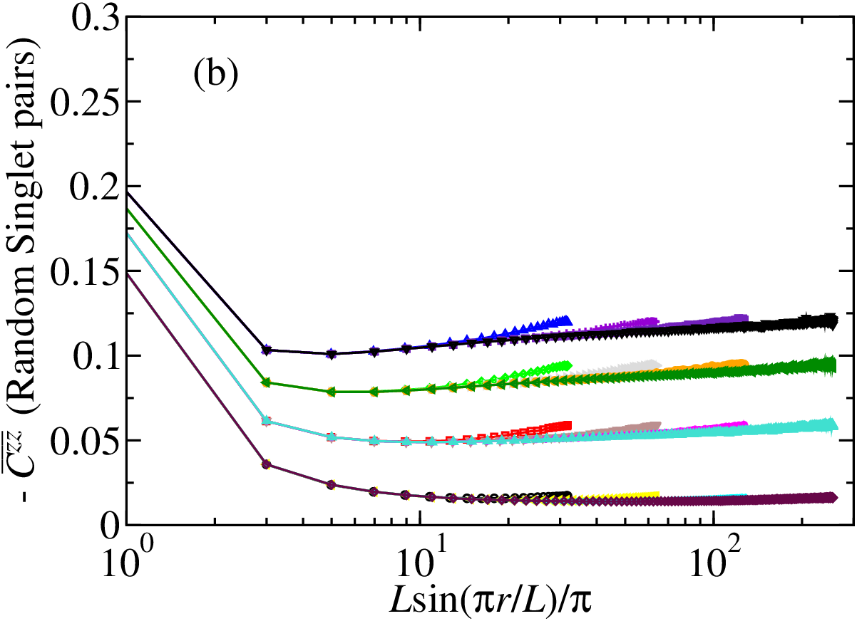
Finally, we would like to call attention for the importance of using quadruple precision and having extra care with the numerical instabilities. Using double precision for and yields to data different from those in Fig. 7. Surprisingly, the observed data (not shown here) exhibits a drop in the correlations (due to the inability of capturing the longest and weakest coupled spin pairs) compatible with a logarithmic correction of type (15) with negative exponent of order , compatible with that reported in Ref. Iglói et al. 2000 [see Eq. (4)]. Since these rare singlets dominate the mean correlations, this means that a spurious logarithmic correction can obtained.
III.2 Typical correlation function and probability distributions
We now turn our attention to the typical value of the spin-spin correlations [as defined in Eq. (6)]. In this study, we report that our data were averaged over distinct disorder realizations.
We start by assuming that, in the long-distance regime , the typical correlations can be well approximated by
| (16) |
where is a disorder-dependent prefactor, represents the crossover function (which for ), is a disorder-independent constant, is the chord length (8), is the Lyapunov exponent (12), and the correction to the chord length is analogous to those for the average correlations (9). Notice that (16) recovers the SDRG prediction of a stretched exponential decay with universal (disorder-independent) and isotropic exponent . Equation (16) assumes that disorder enters in the exponential only via the Lyapunov exponent . While its presence is natural since the stretched exponential form requires a length scale, and thus the corresponding Lyapunov exponent of the underlying single-parameter scaling theory Javan Mard et al. 2014, it is not clear why and should be disorder independent. Nonetheless, as we show below, this hypothesis is compatible with our data. Finally, we mention that, unlike the mean correlations, the numerical prefactor is the same for both even and odd separations .


In Figs. 8(a) and (b) we plot respectively the transverse and longitudinal typical correlations for and various chain sizes and disorder strengths . The insets (i) of those figures bring the raw data from which the SDRG prediction is confirmed.
We then replot the correlations as a function of as shown in the insets (ii) of those figures. Apparently, the constant is disorder-independent. Moreover, the values of used seem to be sufficiently large (at least for ) such that . Therefore, it is safe to obtain the values of and by simply fitting Eq. (16) to our data. 1010 10 We consider only the data such that and . This is simply to ensure some meaning to the fitting function (16) when disorder is weak (). As we explain latter on, this has no influence in our results. The fitting values of and are plotted in Fig. 8(c). For , these are effective values [not in the asymptotic regime , as can be seen in insets (ii)]. The fitting values are consistent with and being disorder independent.
In order to proceed, as in the analysis of the mean correlation , we need the relation between the numerical prefactor and the disorder strength . Clearly, one needs a theory capable of capturing both the clean and the disorder critical behaviors. Here, however, we will simply try to connect the clean behavior (with and ) to the strong-disorder one . Assuming a sharp crossover at , continuity requires that . However, this poorly fits the data in Fig. 8(c). We have tried several modifications of this scenario in order to improve the fit. They include adding one or two polynomials and power-laws , and also changing the prefactor of the logarithmic term. The worst modifications are those in which the logarithmic term is dropped out, implying that is very robust. The most successful modification is such that we admit a sharp crossover happening at . The exponential in the typical correlation then acquires a dependence on yielding to
| (17) |
with , and being fitting parameters. The fitting values are shown in Fig. 8(c) for which only the data for were used. The reason is that for smaller values of , the slope is not fully saturated (due to the effects of the crossover function ). We have checked that changing any of the fitting parameters values by does not change the quality of the fit, i.e., the reduced weighted error sum remains the same within the statistical error. This means that is a reasonable estimate for the accuracy of our fit.
We now put Eq. (17) to test by assuming that it holds for all disorder strengths. In the main panels of Figs. 8(a) and (b), we plot as a function of (recall is fixed). Remarkably, and somewhat surprisingly, we obtain good data collapse even for the least disordered system studied . For small , deviates from the pure stretched exponential, which is attributed to the crossover term . The fact that the data collapse for all disorder strengths means that, to a good approximation, disorder enters in through the combination , i.e., . Once more, this data collapse also supports that is a disorder-independent function.


We are now in the position to study the chord-length-correction function in Eq. (16). In Fig. 9, we plot as a function of suitable combinations of , and . For clarity, we show only a few data such as , with , and , and , , and . As can be seen in the main panel of Fig. 9(a), the chord length is nearly enough for accounting all the finite-size effects. The combination [see the inset of Fig. 9(b)] nearly collapses all the data. The role played by the crossover function and the chord-length-correction function are shown in the main panel of Fig. 9(b). We note that all curves converge to a single one in the large- limit, in agreement with the hypothesis (16). The dashed lines are the best fits restricted to the region and considering only the large system size . The fitting values of and are reported in Fig. 9(b). (Adding higher order terms do not improve our fit.) Notice the small correction to the chord length , much smaller than those for the mean correlations. Interestingly, the crossover function is non-monotonic with respect to . Notice that tends to from above for weak disorder , and from below otherwise. Finally, we verified (not shown) that is nearly a constant for large .


We now turn our attention to the correlation function distribution. In the pioneering work by Fisher, it was conjectured that converges to a non-trivial distribution for large separation . This conjecture was confirmed in Refs. Young and Rieger 1996; Henelius and Girvin 1998 by numerically computing the distribution of for a fixed disorder strength . We confirm this conjecture by studying the distribution of for fixed separation and disorder strength , for various system sizes . As shown in Fig. 10(a) the distribution converges to a non-trivial one for large . According to Eq. (16), the first moment of and converges to the unity in the regime. We first notice that and are not equal. Also, both distributions are narrow. We have tried many different fitting functions. Since they are narrow, we tried Weibull and Gaussian distributions but with poor success. The most satisfactory one is
| (18) |
where is a normalization constant, and , , and are fitting parameters with obvious interpretations. The first term in the exponential dictates the large-distance behavior which, naively, we expect to be near a Gaussian. Then, is the corresponding exponent for the tail, would represent the width and the rescaled offset. The second term dictates the low-distance behavior with corresponding exponent . 1111 11 We also have tried polynomials and verified satisfactory fits with and . Notice that this term represents a sharp cutoff for . We have tried to offset this term via and found that . Surprisingly, our choice of makes the . Our fits extrapolated to are shown as solid lines in Fig. 10(a) and are numerically equal to , , , , , , , , , and .
We now step forward and study how depends on . In Figs. 10(b) and (c) we plot the distribution of (shifted by its average and divided by its standard deviation) for various disorder strengths , system sizes , and separations and . For comparison, we replot the corresponding fits of panel (a) in panels (b) and (c), also shifted by the corresponding mean values (which are both equal to one) and divided by the corresponding standard deviation ( and , respectively for and ). For separations , all distributions are clearly universal, i.e., disorder independent. For shorter separations , the distributions differ from the universal one. Given the systematic tendency towards the universal distribution for larger and larger system sizes , we then attribute this discrepancy to the fact that the limit of large separation has not been achieved for those cases. We therefore conclude that, in the large separation limit, the distribution of converges to a non-trivial, narrow and universal (disorder-independent) distribution.
IV Spin-spin correlations for the correlated coupling constants model
In this section we report our results on the average and typical correlation functions for the case of correlated disorder in the model (1), which is defined by a set of coupling constants (see Sec. II).


Unlike the uncorrelated disorder model, there is no analytical theory predicting the critical exponents. Here, our purpose is to determine them for the average and typical correlation functions.
In Fig. 11, we plot the typical correlations for various chain lengths and disorder strengths and . Clearly, the chord length 8 is almost a perfect scaling variable. 1212 12 Likewise, the chord length was verified to be nearly the correct scaling variable for the Rényi entanglement entropy for any disorder strength Getelina et al. 2016.
Clearly, the typical correlations decay algebraically, which is very distinct from their uncorrelated disorder counterpart. Evidently (not shown here), the average correlations also decays algebraically with the spin separation . Simple fits restricted to the long-distance tail provide the corresponding exponents which are shown in Fig. 12.

For disorder strengths below the threshold , the exponent agrees with those of the clean system , as expected. Tuning the line of finite-disorder fixed points by increasing beyond , the exponents vary continuously and in a non-trivial fashion.
With respect to the transverse correlation, both typical and average exponents are equal within our statistical error, and increase monotonically but is bounded to . This suggests that the distribution of has finite and small width for any distance and system size as can be verified in Figs. 13 and 14.

In contrast, the typical and average longitudinal correlations behave quite differently from each other. The average critical exponent remains equal to the clean one for all disorder strengths studied. The typical one increases linearly for apparently without bounds. This implies that the width of the distribution of increases with , as verified in Fig. 15, but is fixed for and (as we have verified but it is not shown here).


We end this section by calling attention to the striking difference between transverse and longitudinal correlations. Certainly, the ground state is far from the random singlet state of the uncorrelated disorder model. As pointed out in Ref. Getelina et al. 2016, the entanglement properties of the correlated disorder model shares many similarities with the clean ground state. The fact that typical and average longitudinal correlations are quite different points towards less similarities.


V Conclusions
In this work we have studied the spin-spin correlation functions for the quantum critical spin-1/2 XX chain in the case of uncorrelated and correlated coupling constants (see Sec. II). In the former case, the chain is governed by a universal (disorder independent) infinite-randomness fixed point, while in the latter, it is governed by the clean fixed point for weak disorder () and by a line of finite-randomness fixed points tuned by the disorder strength () .
For uncorrelated disorder, we have proposed and numerically verified that the correlations in Eqs. (7), (10), (16) are good approximations in the regime (not restricted to the thermodynamic limit ) for periodic boundary conditions. We have shown that the chord length (8) is not the true scaling variable, exhibiting small corrections for the mean correlations and even smaller for the typical ones. We have parameterized and quantified these corrections through the function in Eq. (9). In principle, these corrections should be non-universal, i.e., disorder dependent. While this may be indeed the case, we could fit our data using the hypothesis that is universal. Naturally, deciding whether is universal or not requires better statistics and larger systems which are out of our current reach.
In addition, we have studied the corresponding non-universal numerical prefactors and linked them to the corresponding Lyapunov exponent (12) which, ultimately, link them to the disorder strength. Surprisingly, we have determined an accurate scaling as quantified in Eqs. (14) and (17) for the mean transverse correlations and the typical longitudinal and transverse correlations, respectively. In general, these prefactors and their scaling with a crossover length depend on the dimensions of the related relevant and irrelevant operators. It is not the scope of the present work to find those operators and their dimensions. We leave this as an open question and hope that our findings serve as future motivation.
We have also studied the distribution of correlations. We have confirmed (not for the first time) the conjecture that the quantity converges to a non-trivial distribution in the large-separation regime. In addition, based on the knowledge built from the typical correlation and its relation with the Lyapunov exponent, we have numerically determined that, in the large separation limit, the distribution of converges to a non-trivial -dependent, narrow and universal (disorder-independent) distribution quantified in Eq. (18).
It is desirable to generalize our results to other anisotropies . It is not entirely clear whether a single-parameter scaling will be possible for all . Assuming that the SDRG method is indeed asymptotically exact in this range of anisotropies, it is then plausible that our results generalize (since under the SDRG flow) at the simple cost of correcting the Lyapunov exponent. Based on the field-theory methods of Ref. Giamarchi and Schulz 1989; Doty and Fisher 1992, it is plausible that Eq. (12) generalizes to , with the Luttinger parameter . Evidently, the values of non-universal quantities such as in (9) may depend on .
Last but not least, we have shown the importance of the finite-size effect and numerical instabilities when characterizing the random-singlet state. They are so strong that can mimic logarithmic corrections to the correct scaling (see Fig. 6).
Conversely, for the correlated disorder model we have shown that the typical correlation functions decay as a power law (see Fig. 11), just like the mean correlations. The corresponding exponents were determined (see Fig. 12) and vary continuously for . While the exponents for the mean and typical transverse correlations remain nearly equal (implying a narrow distribution of correlations), the behavior is strikingly different for the longitudinal correlations, a consequence of the fact that the distribution of longitudinal correlations are much broader. In addition, we have determined the chord length is not the correct scaling variable (but it is a very good approximation to it). The fact that the transverse and longitudinal correlations behave so differently implies that the random-singlet state is far from being a good approximation of the true ground state even when The infinite-randomness low-energy physics of the uncorrelated disorder model is not adiabatically connected to the strong but finite-randomness behavior of the correlated disorder model.
Acknowledgements.
We would like to thank Anders Sandvik and Róbert Juhász for useful discussions, and Nicolas Laflorencie for bringing Ref. Shu et al. 2016 to our attention. This study was financed in part by the Coordenação de Aperfeiçoamento de Pessoal de Nível Superior - Brasil (CAPES) - Finance Code 001, and also by the Brazilian funding agencies CNPq and FAPESP. All authors contributed equally to this work.References
- Ma et al. (1979) S. K. Ma, C. Dasgupta, and C. H. Hu, Phys. Rev. Lett. 43, 1434 (1979).
- Dasgupta and Ma (1980) C. Dasgupta and S. K. Ma, Phys. Rev. B 22, 1305 (1980).
- Bhatt and Lee (1982) R. N. Bhatt and P. A. Lee, Phys. Rev. Lett. 48, 344 (1982).
- Iglói and Monthus (2005) F. Iglói and C. Monthus, Phys. Rep. 412, 277 (2005).
- Iglói and Monthus (2018) F. Iglói and C. Monthus, The European Physical Journal B 91, 290 (2018).
- Fisher (1992) D. S. Fisher, Phys. Rev. Lett. 69, 534 (1992).
- Fisher (1994) D. S. Fisher, Phys. Rev. B 50, 3799 (1994).
- Vojta (2006) T. Vojta, J. Phys. A: Math. Gen. 39, R143 (2006).
- Doty and Fisher (1992) C. A. Doty and D. S. Fisher, Phys. Rev. B 45, 2167 (1992).
- Laflorencie et al. (2004) N. Laflorencie, H. Rieger, A. Sandvik, and P. Henelius, Phys. Rev. B 70, 054430 (2004).
- Hoyos and Rigolin (2006) J. A. Hoyos and G. Rigolin, Phys. Rev. A 74, 062324 (2006).
- Hoyos et al. (2007) J. A. Hoyos, A. P. Vieira, N. Laflorencie, and E. Miranda, Phys. Rev. B 76, 174425 (2007).
- Ristivojevic et al. (2012) Z. Ristivojevic, A. Petković, and T. Giamarchi, Nucl. Phys. B 864, 317 (2012).
- Shu et al. (2016) Y. R. Shu, D. X. Yao, C. W. Ke, Y. C. Lin, and A. W. Sandvik, Phys. Rev. B 94, 1 (2016).
- Getelina et al. (2018) J. C. Getelina, T. R. de Oliveira, and J. A. Hoyos, Physics Letters A 382, 2799 (2018).
- Shu et al. (2018) Y.-R. Shu, M. Dupont, D.-X. Yao, S. Capponi, and A. W. Sandvik, Phys. Rev. B 97, 104424 (2018).
- Theodorou (1977) G. Theodorou, Phys. Rev. B 16, 2264 (1977).
- Masuda et al. (2004) T. Masuda, A. Zheludev, K. Uchinokura, J.-H. Chung, and S. Park, Physical Review Letters 93, 077206 (2004).
- Shiroka et al. (2013) T. Shiroka, F. Casola, W. Lorenz, K. Prša, A. Zheludev, H.-R. Ott, and J. Mesot, Phys. Rev. B 88, 054422 (2013).
- Shiroka et al. (2019) T. Shiroka, F. Eggenschwiler, H.-R. Ott, and J. Mesot, Phys. Rev. B 99, 035116 (2019).
- Lieb et al. (1961) E. Lieb, T. Schultz, and D. Mattis, Ann. Phys. 16, 407 (1961).
- McCoy (1968) B. M. McCoy, Phys. Rev. 173, 531 (1968).
- Luther and Peschel (1975) A. Luther and I. Peschel, Phys. Rev. B 12, 3908 (1975).
- Haldane (1980) F. D. M. Haldane, Phys. Rev. Lett. 45, 1358 (1980).
- Giamarchi and Schulz (1989) T. Giamarchi and H. J. Schulz, Phys. Rev. B 39, 4620 (1989).
- Singh et al. (1989) R. R. P. Singh, M. E. Fisher, and R. Shankar, Phys. Rev. B 39, 2562 (1989).
- Hallberg et al. (1995) K. A. Hallberg, P. Horsch, and G. Martínez, Phys. Rev. B 52, R719 (1995).
- Lukyanov and Zamolodchikov (1997) S. Lukyanov and A. Zamolodchikov, Nucl. Phys. B 493, 571 (1997).
- Affleck (1998) I. Affleck, Journal of Physics A: Mathematical and General 31, 4573 (1998).
- Lukyanov (1998) S. Lukyanov, Nuclear Physics B 522, 533 (1998).
- Hikihara and Furusaki (1998) T. Hikihara and A. Furusaki, Phys. Rev. B 58, R583 (1998).
- Lukyanov (1999) S. Lukyanov, Phys. Rev. B 59, 11163 (1999).
- Hoyos et al. (2011) J. A. Hoyos, N. Laflorencie, A. P. Vieira, and T. Vojta, EPL Europhysics Lett. 93, 30004 (2011).
- Getelina et al. (2016) J. C. Getelina, F. C. Alcaraz, and J. A. Hoyos, Phys. Rev. B 93, 045136 (2016).
- Macdiarmid et al. (1987) A. Macdiarmid, J. Chiang, A. Richter, and A. Epstein, Synthetic Metals 18, 285 (1987).
- Dunlap et al. (1990) D. H. Dunlap, H.-L. Wu, and P. W. Phillips, Phys. Rev. Lett. 65, 88 (1990).
- Wu and Phillips (1991) H.-L. Wu and P. Phillips, Phys. Rev. Lett. 66, 1366 (1991).
- Quito et al. (2015) V. L. Quito, J. A. Hoyos, and E. Miranda, Phys. Rev. Lett. 115, 167201 (2015).
- Quito et al. (2020) V. L. Quito, P. L. S. Lopes, J. A. Hoyos, and E. Miranda, Eur. Phys. J. B 93, 17 (2020).
- Quito et al. (2019) V. L. Quito, P. L. S. Lopes, J. A. Hoyos, and E. Miranda, Phys. Rev. B 100, 224407 (2019).
- Hamacher et al. (2002) K. Hamacher, J. Stolze, and W. Wenzel, Phys. Rev. Lett. 89, 127202 (2002).
- Henelius and Girvin (1998) P. Henelius and S. M. Girvin, Phys. Rev. B 57, 11457 (1998).
- Iglói et al. (2000) F. Iglói, R. Juhász, and H. Rieger, Phys. Rev. B 61, 552 (2000).
- Xavier et al. (2018) J. C. Xavier, J. A. Hoyos, and E. Miranda, Phys. Rev. B 98, 195115 (2018).
- Rieger and Iglói (1999) H. Rieger and F. Iglói, Phys. Rev. Lett. 83, 3741 (1999).
- Ibrahim et al. (2014) A. K. Ibrahim, H. Barghathi, and T. Vojta, Phys. Rev. E 90, 042132 (2014).
- Affleck et al. (1989) I. Affleck, D. Gepner, H. J. Schulz, and T. Ziman, J. Phys. A22, 511 (1989).
- Fagotti et al. (2011) M. Fagotti, P. Calabrese, and J. E. Moore, Phys. Rev. B 83, 1 (2011).
- Javan Mard et al. (2014) H. Javan Mard, J. A. Hoyos, E. Miranda, and V. Dobrosavljević, Phys. Rev. B 90, 125141 (2014).
- Young and Rieger (1996) A. Young and H. Rieger, Phys. Rev. B 53, 8486 (1996).