Inferring entropy production from short experimentsPreprint: APS/123-QED

A fundamental property of non-equilibrium systems is the existence of currents which are fueled by a non vanishing average rate of total entropy production $\sigma:=\langle\Delta S_{tot}\rangle/\tau$, where $\tau$ is the time interval over which we observe the system. An estimate of $\sigma$ quantifies how much heat is dissipated to the environment on average or how much free energy is lost per unit time. More information is available from fluctuations of $\Delta S_{tot}$. These are governed by the fluctuation theorems Evans-Cohen; Evans-Searles; Searles-Evans; Searles2001; Gallavotti-Cohen; Gallavotti1995; Kurchan; Lebowitz-Spohn; JarzynskiPRL; crooks; Seifert:2012stf; Seifert:2005epa and can be used for the estimation of free energy differences and hummer2001free; liphardt2002equilibrium studying the binding energies in single-molecule Mossa_2009; ritort2006single or multi-molecular experiments camunas:ebe. An accurate quantification of the statistics of $\Delta S_{tot}$ could also help improve our understanding of the non-equilibrium physics of active matter systems Ramaswamy:MSA, biological systems Cates_2012; seara2018entropy and nanoscale devices Pietzonka:2018utp; Manikandan:EF; Verley:2014uce; Verley:2014ute such as colloidal heat engines Martinez:2017che; Martinez:2016bce.

The main challenge in the thermodynamic characterization of microscopic systems continues to be however, the lack of a general scheme for the measurement and characterization of $\Delta S_{tot}$. For systems such as colloidal particles, for which the full dynamical equations are known, stochastic thermodynamics provides a framework to quantify $\Delta S_{tot}$ from individual trajectories sekimoto1997kinetic; sekimoto1998langevin; Seifert:2012stf. For more complex systems where not all relevant mesostates are accessible, these direct strategies fail Seifert:inf; martinez2019inferring. The only options are either to perform local calorimetric measurements to directly measure the heat emitted to the bath basta2018sensitive or to come up with a new scheme for inferring $\sigma$ indirectly.

Recently, for non-equilibrium systems in a steady state, such a scheme for identifying $\sigma$ has been proposed Seifert:inf; Gingrich:qua using the thermodynamic uncertainty relation PhysRevLett.114.158101; barato:ubo. Using this scheme, a lower bound $\sigma_{L}$ for $\sigma$ can be obtained from the measurement of any fluctuating current $J$, in terms of its mean $\left\langle J\right\rangle$ and variance $\text{Var}(J)$ as,

Here, $k_{B}$ is the Boltzmann constant. Eq. (1) holds for arbitrary $\tau$ for non-equilibrium systems in a steady state Seifert:ftg, and the proof follows from a $\sigma$-dependent parabolic bound on the large deviation function Touchette:2009lda of $J$ Ginrich:dba; gingrich:pft.

This inference scheme for $\sigma$ has been shown Gingrich:qua to perform better than more direct methods that use spatial or temporal averages. However, since the uncertainty relation is an inequality, Eq. (1) still only gives a bound for $\sigma$ even when $J=\Delta S_{tot}$. How tight this bound is depends in general on model details and the $J$ chosen. As a result, there has been much interest recently on how to choose $J$ such that the bound value is the tightest Gingrich:qua; Pigolotti:hac. For $\tau\rightarrow\infty$, it is known that the current $J$ that gives the best bound is $J=\Delta S_{tot}$ Ginrich:dba.

Eq. (1) could be used to predict $\sigma$ exactly if the equality was to hold. One case when this is known to happen is the equilibrium limit PhysRevLett.114.158101; Ginrich:dba; Manikandan:2018erf with $J=\Delta S_{tot}$. This means, that for systems working in the close-to-equilibrium/linear response regimes, there is a possibility to estimate $\sigma$ arbitrarily close to the exact value by using Eq. (1). The equality in Eq. (1) is also met for arbitrary non-equilibrium conditions if along with $J=\Delta S_{tot}$, certain conditions are met by the steady state current and probability distributions hasegawa:pre; Physical. However, there is no general scheme available so far for inferring sigma exactly under arbitrary non-equilibrium conditions. In addition no scheme exists, to our knowledge, for inferring fluctuations in $\Delta S_{tot}$.

We address precisely these issues in this Letter. Our first central contribution is to provide a new strategy which, in principle, can estimate $\sigma$ exactly at arbitrary non-equilibrium conditions, by using Eq. (1) in the $\tau\rightarrow 0$ limit. In this limit, for the current $J=\Delta S_{tot}$, it can be shown that the equality condition holds, just as for the equilibrium limit. Using this feature, we show that we can infer $\sigma$ arbitrarily close to the exact value, by evaluating $\sigma_{L}$ for a variety of $J$ calculated over very short time durations, and then choosing the largest value of $\sigma_{L}$ that results. A particularly appealing point from an experimental perspective is that, since we need to only compute $\sigma_{L}$ of Eq. (1) over very short trajectories, a single long time-series could suffice to obtain both $\langle J\rangle$ and Var$(J)$. Notice that the value of $\sigma$ so inferred is the steady-state value and hence valid at all times.

Our second contribution is to demonstrate that, by combining the value of $\sigma$ inferred from the previous step and the structure of the large deviation function of arbitrary currents Ginrich:dba; Pietzonka:ubo; gingrich:pft, we can also infer the distribution of $\Delta S_{tot}$, and as a result all the cumulants, arbitrarily close to their exact values. We illustrate all our findings using exact and numerical solutions for two models of colloidal engines, namely the Brownian gyrator Filliger:2007bgm; Manikandan:EF as well as the isothermal work-to-work converter engine Gupta:2017sei.

We begin by considering the uncertainty relation for $J=\Delta S_{tot}$, which reads (setting $k_{B}=1$),

To motivate that this inequality saturates at $\tau\rightarrow 0$, we consider the arbitrary time, scaled cumulant generating function (SCGF) $\phi_{\Delta S_{tot}}(\lambda,\tau)\equiv\frac{1}{\tau}\log\left\langle e^{-\lambda\Delta S_{tot}}\right\rangle_{\tau}$. For short time durations, when $|\Delta S_{tot}|\ll 1$, we can express $\phi_{\Delta S_{tot}}(\lambda,\tau)$ as a series expansion in terms of the cumulants of $\Delta S_{tot}$. Then, to the leading order that respects convexity, we get (see the Supplemental Material suppl for more details and explicit expressions for the first four cumulants for an exactly solvable model),

Now applying the integral fluctuation theorem Seifert:2005epa: $\phi_{\Delta S_{tot}}(1,\tau)=0$, we get,

We stress that the limit $\tau\rightarrow 0$ is crucial for Eq. (3) and Eq. (4) to hold. For an arbitrary $\tau$ they are valid only if the distribution of $\Delta S_{tot}$ is a Gaussian. A more rigorous proof is provided in hasegawa:turfc to the effect that the equality in Eq. (2) is always attained when $\Delta S_{tot}\rightarrow 0$. However, note for our purposes, that this happens not only for the equilibrium limit but also when $\tau\rightarrow 0$. A model which can be solved exactly for the LHS of Eq. (2) has also been shown Manikandan:2018erf to display this behaviour as $\tau\rightarrow 0$.

We now demonstrate the usefulness of Eq. (4) for inferring $\sigma$ for two non-trivial models of colloidal engines, the Brownian gyrator model Filliger:2007bgm; Argun:2017erm; Manikandan:EF and the work-to-work converter engine Gupta:2017sei; Manikandan:EF, in both of which the working substance is a single colloidal particle. In the first case, the particle is in contact with external reservoirs at hot ($T_{1}$) and cold ($T_{2}$) temperatures and in the second case, the particle is subjected to two white-noise forces, interpreted as a load and drive force. In these models, there is a clear division of $\Delta S_{tot}$ in terms of time-extensive quantities such as heat ($Q$) and work ($W$) and time-intensive contributions such as the entropy change of the system $\Delta S_{sys}$. Hence $\Delta S_{tot}$ can be written as,

Here $\eta_{C}=1-\frac{T_{2}}{T_{1}}$, is the Carnot efficiency.

The term $\Delta S_{int}=-\frac{1}{T_{2}}\Delta E+\Delta S_{sys}$ collects the time-intensive contributions to the total entropy production that depend only on the initial and final states of the system. $\Delta E$ denotes the change in internal energy, which is, according to the First Law, $\Delta E=W+Q_{1}+Q_{2}$. We define an arbitrary current $J$ in the system as the linear combination $J=c_{1}\;\frac{\eta_{C}}{T_{2}}Q_{1}+c_{2}\;\frac{1}{T_{2}}W+c_{3}\;\Delta S_{int}$, where $c_{1},\;c_{2}$ and $c_{3}$ are random real numbers, taken uniformly from the interval $\left[-1,\;1\right]$. In particular, when $c_{1}=c_{2}=c_{3}=1$, we get $J=\Delta S_{tot}$ ¹¹ 1 In principle, one can also consider any arbitrary decomposition of $\Delta S_{tot}$ with more components. We will stick to a three dimensional basis for simplicity..

In Fig. 1 we illustrate this inference scheme for the Brownian gyrator (Fig. 1, left panel) and the work-to-work converter engine (Fig. 1, right panel). Since both of these models have been extensively studied in the literature, we relegate their detailed description to the Supplemental Material suppl. The Brownian gyrator can be solved exactly Manikandan:EF for the full SCGF $\Phi(\lambda_{Q},\lambda_{w},\lambda_{S},\tau)\equiv\frac{1}{\tau}\log\left\langle e^{-\lambda_{Q}Q_{1}-\lambda_{W}W+\lambda_{S}\Delta S_{int}}\right\rangle_{\tau}$ at arbitrary times and hence provides us with the means to check the inference procedure analytically (see the Supplemental Material suppl, which also contains the references Manikandan:2017awd; Chernyak:2006pia; Onsager:1953fai; Machlup:1953fai; Kirsten:2003fdc ). The second model of the work-to-work converter can only be solved for large times Gupta:2017sei. We hence use it to test our inference scheme in a situation where we can only rely on numerics.

In the left panel of Fig. 1, we compute $\sigma_{L}$ for the Brownian gyrator, using our analytical solutions (see suppl for more details) for arbitrary currents $J$ at any time $\tau$. The exact value of $\sigma$ is marked by the black horizontal line. In the $\tau\rightarrow 0$ limit, $\Delta S_{tot}$ infers $\sigma$ exactly. Also, notice that there are other currents which perform almost as good as $\Delta S_{tot}$, and infer $\sigma$ arbitrarily close to the actual value, in the $\tau\rightarrow 0$ limit. The red solid lines correspond to a value of $\sigma_{L}$ computed from currents for which $c_{3}\neq 0$. The blue dotted lines correspond to $\sigma_{L}$ calculated from currents for which $c_{3}=0$ and hence which are only linear combinations of $Q_{1}$ and $W$, the time-extensive contributions to $\Delta S_{tot}$. The best inference strategy is therefore to measure the mean and variance of an ensemble of randomly generated currents, at short times. Since, the bound in Eq. (1) saturates for $\tau\rightarrow 0$, we are guaranteed to obtain a value for $\sigma_{L}$ arbitrarily close to the actual $\sigma$ as,

Note that for large $\tau$ all currents, including $J=\Delta S_{tot}$ give a similar estimate, which is considerably less than the actual value (left panel, Fig. 1). Hence, the small-time saturation of Eq. (1) as well as it’s sensitivity to the chosen $J$, both work in favour of getting a better estimate for $\sigma$ than at large $\tau$. In practice, the $\tau\rightarrow 0$ limit may be achieved in experiments by choosing trajectory lengths corresponding to the minimal temporal resolution accessible to the experiment kheifets2014observation; di2014probing such that $\Delta S_{tot}$ also becomes arbitrarily small in this limit. In the right panel of Fig. 1, we numerically compute $\sigma_{L}$ for the second model of the work-to-work converter, by computing the mean and variance of different randomly chosen $J$ for very short trajectories and using Eq. (6). Since this model can be solved in the steady state Gupta:2017sei, the exact value of $\sigma$ is known. As can be seen, the inferred value is in very good agreement with the exact value after the inference procedure has been applied to the order of about $20$ currents.

To further analyze the inference of $\sigma$ by the short-time inference scheme, Eq. (6), we have identified the optimal currents that infer $\sigma$ the best. In Fig. 2, we illustrate this in the $\tau\rightarrow 0$ limit for the Brownian gyrator. When $c_{3}\;\neq 0$ the current that infers best is $\Delta S_{tot}$ itself, as expected. However, for $c_{3}=0$, some other direction in the $(c_{1}$, $c_{2})$ plane gives the current that infers best (Fig. 2).

Even when $\tau>0$ , we find (see Supplemental Material suppl), that the optimal current is in general different from $\Delta S_{tot}$ as recently suggested in Pigolotti:hac, and becomes equal to $\Delta S_{tot}$ only for large $\tau$ Ginrich:dba.

It is important to note that, our usage of the $c_{1},c_{2},c_{3}$ -space is purely a proof of concept, to demonstrate the viability and applicability of our short-time inference scheme, as well as to disentangle the separate roles played by the time-intensive and time-extensive terms which would not have been obvious otherwise. In addition, in this space, currents have natural physical interpretations in terms of work, heat and system entropy production. For a generic non-equilibrium system however, for which neither a Langevin nor a Master equation description is known, such a decomposition of $\Delta S_{tot}$ (Eq. (5)) is usually not possible. In such cases, one can generate random currents from the phase space trajectories $\textbf{x}(t)$ of the system Gingrich:inf; Gingrich:qua using random vectors $\textbf{d}(\textbf{x})$ as $J\equiv J_{d}=\int_{\textbf{x}(0)}^{\textbf{x}(\tau)}d\textbf{x}\;\textbf{d}(\textbf{x})\;\textbf{j}(\textbf{x})$, where $\textbf{j}(\textbf{x})=\frac{1}{\tau}\int_{0}^{\tau}\delta[\textbf{x}-\textbf{x}(t)]\;d\textbf{x}(t)$ is an estimate for a steady state current. Such a current can then be used to compute $\sigma_{L}$ in Eq. (1) and many such currents can be generated by varying d. Our scheme will then imply that as $\tau\rightarrow 0$, the current that will satisfy the equality in Eq. (1) will correspond to $\Delta S_{tot}$. Note that $J_{d}$’s defined this way contain information of both the extensive and intensive contributions and there is no need to calculate the steady state distribution separately. In the Supplemental Material, we show the d field which corresponds to $J=\Delta S_{tot}$ for the Brownian gyrator. For problems where an analytical treatment is ruled out, such a d field would have to be obtained by some optimisation procedure Gingrich:qua.

So far, we have shown that the finite time thermodynamic uncertainty relation can be used at very short observational times to infer $\sigma$ arbitrarily close to the actual value, arbitrarily far from equilibrium. It is then natural to ask, if there exist similar inference strategies for the fluctuations of $\Delta S_{tot}$ as well. Since the current that infers $\sigma$ the best at $\tau=0$ is $J=\Delta S_{tot}$, a naive solution would have been to approximate the optimal current in the $\tau\rightarrow 0$ limit by $\Delta S_{tot}$, and compute a distribution directly from that. Although this can work in principle, there are a couple of practical disadvantages. First, with the real data, one is always limited by the minimal experimental resolution $\Delta t>0$ and the $\tau\rightarrow 0$ limit can be accessed only within this error. Secondly, there can be several near optimal currents (as shown in Figure. 1, Left) that infer $\sigma$ arbitrarily close to the exact value, which a computational scheme may not be able to distinguish. For e.g., it has been noticed in Gingrich:qua, for finite $\tau$, that these near optimal currents can look very different from each other, and still predict a similar value for $\sigma$. As a result of these limitations, because of which we may have access to a value $\sigma$, but not the current $J=\Delta S_{tot}$, we present an alternate strategy for computing the steady state distribution of $\Delta S_{tot}$ using an exact estimate of $\sigma$.

We begin by considering the structure of the scaled cumulant generating function of an arbitrary current in the steady state, $\phi^{\sigma}_{J}(\lambda,\tau)\equiv\frac{1}{\tau}\log\left\langle e^{-\lambda\frac{\sigma\tau J}{\left\langle J\right\rangle}}\right\rangle_{\tau}$ at large $\tau$. Using large deviation techniques, it has been shown recently that $\phi^{\sigma}_{J}$ obeys the bound Pietzonka:ubo; Ginrich:dba,

The uncertainty relation in Eq. (1) can be directly proved from this result Ginrich:dba; gingrich:pft. Interestingly, Eq. (7) constrains the fluctuations of $\Delta S_{tot}$ strongly, by providing both a lower bound and an upper bound for $\phi_{\Delta S_{tot}}$. In particular, one can saturate the bound $\phi_{\Delta S_{tot}}(\lambda,\tau)\leq\phi^{\sigma}_{J}(\lambda,\tau)$ if $J=\Delta S_{tot}$. We therefore get a natural scheme for inferring $\phi_{\Delta S_{tot}}(\lambda,\tau)$ as,

Consequently, if $M_{J}^{(n)}$ is the $n$-th cumulant of the normalized current $\sigma\tau J/\langle J\rangle$, we also get (see suppl),

The cumulants thus inferred can then be used to construct the histogram of $\Delta S_{tot}$ straightforwardly.

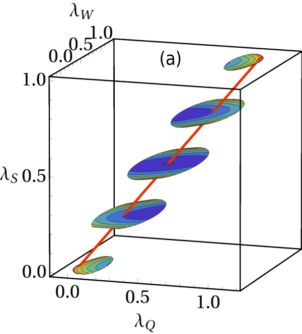
We illustrate Eqs. (8) and (9) in Fig. 3 for the isothermal work-to-work converter engine. We have first obtained an analytic expression for the joint SCGF $\Phi(\lambda_{Q},\lambda_{W},\lambda_{S},\tau)=\frac{1}{\tau}\log\langle e^{-\frac{\lambda_{Q}\eta_{C}Q_{1}}{T_{2}}-\frac{\lambda_{W}W}{T_{2}}-\lambda_{S}\,\Delta S_{int}}\rangle_{\tau}$, which is exact at large but finite times (see the Supplemental Material suppl). The geometry of $\Phi$ was recently conjectured and discussed in some detail in Manikandan:EF. Due to the fluctuation theorem, $\Phi$ is a reflection symmetric object around the point $(0.5,0.5,0.5)$, and typically has a limited domain of convergence (cut-offs) that depend on $\lambda_{S}$. We illustrate this for a fixed, large value of $\tau$ in Fig. 3a. The SCGF of an arbitrary current $J$ can be obtained from $\Phi$ by evaluating it along a straight line passing through the origin and the point $\left(c_{1},c_{2},c_{3}\right)$, where $c_{1}$, $c_{2}$, $c_{3}$ are random numbers. In particular, $\phi_{\Delta S_{tot}}$ is $\Phi$ evaluated along the (1,1,1) direction marked by the red solid line in Fig. 3a.

In Figs. 3b and 3c, we illustrate the inference of $\phi_{\Delta S_{tot}}$ using Eq. (8). Since $\phi^{\sigma}_{J}$ of currents with $c_{3}=0$, can have restricted domains of convergences (see $\lambda_{S}=0$ plane of Fig. 3a), they will end up inferring a limited domain of $\phi_{\Delta S_{tot}}$, as shown in Fig. 3c with the blue circles. The red squares show the improvement in the estimate of $\phi_{\Delta S_{tot}}$ when $c_{3}\neq 0$. In Fig. 3d, we illustrate the inference of Var$(\Delta S_{tot})$ using Eq. (9), numerically.

In summary, we have presented a scheme to exactly infer the average entropy production rate $\sigma$ as well as the distribution of entropy production $P(\Delta S_{tot})$ in non-equilibrium steady state systems. The scheme for identifying $\sigma$ is built upon the finite time thermodynamic uncertainty relation gingrich:pft; Seifert:ftg and it’s saturation in the very short time limit. The inference of $P(\Delta S_{tot})$ is then built upon an exactly estimated value of $\sigma$ and the dissipation bounded structure of steady state current fluctuations Pietzonka:ubo; Ginrich:dba.

We have chosen to demonstrate our scheme using a decomposition of $\Delta S_{tot}$ into time-extensive and intensive contributions, but we expect that our scheme is equally applicable for currents generated any other way. Such considerations will be very relevant when testing this scheme in biological systems or active matter systems in the steady state. Generalizations to time symmetrically driven systems hasegawa:turfc could also be interesting.

Note added: Recent preprints otsubo2020estimating; van2020entropy have independently found further proofs/refinements of the short-time inference scheme, and have proposed efficient computational algorithms to implement it.