Inverse design of light-matter interactions
Abstract
Inverse design represents a paradigm shift in the development of nanophotonic devices, where optimal geometries and materials are discovered by an algorithm rather than symmetry considerations or intuition. Here we present a very general formulation of inverse design that is applicable to atomic interactions in external environments, and derive from this some explicit formulae for optimisation of spontaneous decay rates, Casimir-Polder forces and resonant energy transfer. Using the Purcell factor of latter as an example, we use finite-difference time-domain techniques to demonstrate the ability of inverse design algorithms to go far beyond what can be achieved by intuition-based approaches, opening up a new route to their technological exploitation.
Traditional design methods work by specifying a device, then investigating its properties. By contrast, in inverse design the desired property is specified, and an algorithm is left to find a device which fulfils the desired criteria. A naive approach to this would be simply trying all devices that fulfil some set of design constraints. The large space of possible designs renders this numerically unrealistic, meaning that a pre-determined set of designs must be optimised over, at least in the earliest applications of inverse methods to electromagnetic problems Spuhler et al. 1998; Dobson and Cox 1999. The development of adjoint methods Jameson 1988 originally used in aerodynamics have made unconstrained inverse design computationally feasible, with the first application in photonics being to low-loss waveguide bends Jensen and Sigmund 2004. Adjoint methods were subsequently applied to band gaps Kao et al. 2005, solar cells Alaeian et al. 2012, on-chip demultiplexers Piggott et al. 2015 and many more diverse systems — see the recent review articles Jensen and Sigmund 2011; Molesky et al. 2018 and references therein.
An area in which inverse design has not yet been applied is virtual-photon mediated interactions, such as Casimir-Polder Casimir and Polder 1948 forces and resonant energy transfer Förster 1948. These processes can be described within a very general formalism known as macroscopic quantum electrodynamics (QED) Gruner and Welsch 1996, where they can be reduced to various functionals of the classical dyadic Green’s tensor for a source at , observation point at and frequency defined to satisfy
| (1) |
subject to given boundary conditions. The quantised electromagnetic fields can be found from this, for example the electric field in a region with permittivity and unit permeability is given by Gruner and Welsch 1996, where are a set of bosonic creation and annihilation operators for the medium-assisted quantised electromagnetic field11 1 These are usually called and in macroscopic QED, here we avoid that notation in order to avoid confusion with the merit functions introduced later.. The Green’s tensor takes into account both the geometry and material response of an arbitrarily-shaped medium, meaning that an optimal geometry for particular and is represented by a particular functional form of . It follows that is the fundamental object which is to be worked with in inverse design of macroscopic QED.
In this Letter we begin by introducing the underlying formulae for inverse design of light-matter interactions. We then use the specific example of resonant energy transfer combined with finite-difference time domain (FDTD) techniques to demonstrate that the efficiencies achievable in this method are far beyond those found from ‘by-hand’ constructions, opening up a new direction in the design of any light-matter interaction dependent device.
General formulation.
In order to carry out any optimisation, we need to define a merit function which we intend to maximise. In traditional presentations of adjoint optimisation, this function is taken to depend on the electromagnetic fields and , but all of these are of course deducible from the dyadic Green’s tensor so we consider as being dependent on only . The merit function should be an observable quantity, so we take it to be a real-valued functional of , integrated over all its arguments:
| (2) |
The integrals allow us to take into account a delocalised source and extended observation volume, as well as multi-mode effects. The entries of the tensor are in general complex-valued, so in principle one could consider variations in the real and imaginary parts separately. However, it is more convenient to consider the complex tensors and as independent, in which case the variation of the merit function with is;
| (3) |
where represents the Frobenius product () and is a change in the Green’s function brought about by an infinitesimal change in the environment. If this change can be considered as being confined to a small volume containing a number density of atoms with polarisabilities , we can write in terms of the following Born series;
| (4) |
where is the vacuum permeability. The change in the merit function is then given by;
| (5) |
where Lorentz reciprocity has been used. Merit functions for observables that depend on can be obtained via the replacements and .
There are several features of (General formulation.) worth commenting on. In traditional presentations of adjoint optimisation, the equivalent of (General formulation.) is represented as the product of two electric fields. The first is the ‘direct’ field, which is simply the electric field induced by the sources present in the system. The second is the adjoint field, which is that generated by a dipole oscillator at the observation point with an amplitude given by the electric-field derivative of the merit function. The advantage of adjoint methods is that the optimal value of the merit function can be found with only two simulations (rather than a brute force method entailing placement of a dielectric inclusion at each possible point in the optimisation region and repeatedly simulating for each). This is reflected our version of the merit function change shown in (General formulation.); once the two independent Green’s tensors for a source at and a source at in a given environment (e.g. vacuum) have been calculated, is known at all points. The link with the adjoint electric field is simply that one of the Green’s tensors in (General formulation.) has been transposed.
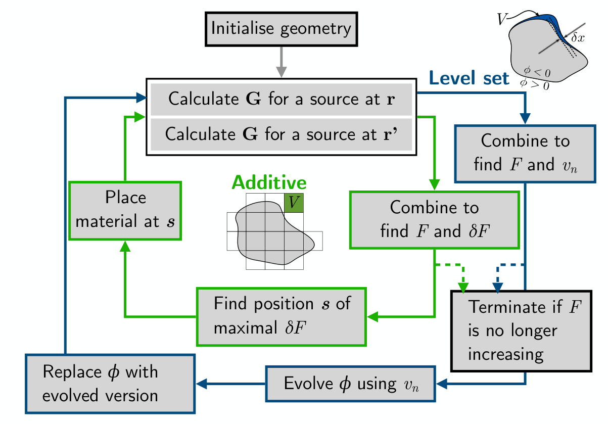
At this point one has at least two choices for how to practically implement an optimisation — the simplest is an additive scheme illustrated in the center of Fig. 1. Here a small block of material is added at the point of maximal , then the two Green’s tensors in the new geometry are recalculated and combined to find a the next optimal point, an so on as indicated in Fig. 1.
The second way to implement the optimisation consists of gradually optimising the shape of an initial object by changing its boundary, known as the level-set method Osher and Sethian 1988. This takes advantage of the fact that (General formulation.) avoids any explicit reference to electric or magnetic fields, thereby avoiding complications with the discontinuities usually found when the fields either side of boundary need to be considered, rather including them in the Green’s tensor itself. Here, the initial boundary shape (as well as its subsequent evolution) is encoded by a chosen function . This is defined as negative inside the boundary, zero on it and positive outside, as indicated in Fig. 1. Introducing a ‘time’ parameter representing iteration, one is led to the following equation of motion governing the shape of the boundary Osher and Sethian 1988: where is the velocity of motion normal to the surface. Formally, this is an advection equation which can be solved using techniques from fluid dynamics. Taking the volume in (General formulation.) to be that defined by the function , we can let; where the shape deformation has been assumed to be small, as can be ensured by a sufficiently small time step in the evolution process. If the integrand of the integral in (General formulation.) is positive at each iteration, the value of the merit function will continually increase. Positivity of (General formulation.) can then be ensured by using a velocity such that , which means identifying;
| (6) |
This velocity can be directly calculated for a given , then inserted into the advection equation, after which is evolved for . This delivers a new , which defines a new geometry, for which we can calculate the new and the process iterates.
Equation (General formulation.) can be directly applied to any quantity that can be expressed in terms of the Green’s dyadic . This includes Casimir Casimir 1948; Raabe et al. 2003 and Casimir-Polder forces Casimir and Polder 1948; Buhmann et al. 2004a, spontaneous decay (Purcell factor) Purcell 1946; Joulain et al. 2003, quantum friction Pendry 1997; Klatt et al. 2017, interatomic Coulombic decay Cederbaum et al. 1997; Hemmerich et al. 2018, radiative heat transfer Polder and Van Hove 1971; Volokitin and Persson 2001, van der Waals forces Buhmann et al. 2004b, non-linear optical processes Lindel et al. 2019 and many more (the latter reference for each of these is where the formula in terms of can be found). The merit functions for a selection of these are shown in Table 1.
![[Uncaptioned image]](1910.00389v2/Table.png)
Example implementation:
In order to demonstrate the application of (General formulation.), we make some simplifying assumptions. We assume that the dielectric additions are homogenous and sufficiently small that the integral over can be approximated by the value at its centre :
| (7) |
In practice, quantities which depend on the field at a single frequency and at a single position are considerably more computationally tractable than their multi-frequency, bulk medium counterparts. Here we concentrate on a simple and universal phenomenon which is well-approximated by radiation of a single frequency interacting with a point-like atom — resonant energy transfer (RET). Extension to bulk media would not involve too much extra computational overhead since this would still only require two Green’s tensors, but calculations of quantities dependent on a continuous spectrum (e.g. ground-state Casimir-Polder forces) would require re-calculation of at very many frequencies. Our Green’s tensor-based method can also be applied to nonlinear processes such as sum- or frequency-difference generation Lindel et al. 2019
We will work in the dipole approximation and aim to optimise the RET rate between dipole moments and , meaning we take;
| (8) |
We then have simply;
| (9) |
which is the well-known of resonance energy transfer rate . Using this in (Example implementation:), after some algebra one finds
| (10) |
which is the equation we will work with from here on.
In order to demonstrate the main features of the method we restrict ourselves to systems with translational invariance along one axis, meaning they can be considered as effectively two-dimensional. In order to validate the two-dimensional RET results that we will calculate (as well as the general FDTD approach), it is necessary to have an analytic expression for RET in two dimensions. Formally, 2D-RET is equivalent to taking a pair of ‘line dipoles’ each consisting of two infinitely extended parallel oppositely-charged wires in three dimensions, as discussed in detail in Martin and Piller 1998. The Green’s tensor from Martin and Piller 1998 can be directly substituted into (9), resulting in a lengthy expression, which can be simplified by noting that in situations of practical interest the dipoles are often randomly oriented necessitating an isotropic average, which gives;
| (11) |
where and are Hankel functions of the first and second kind respectively, and . (Example implementation:) can be used to validate our general FDTD, see Fig. 2.
We can now calculate the effect of arbitrary 2D geometries on RET by examining the dimensionless Purcell factor , where is the rate in vacuum. We initially choose some geometries which are expected to enhance RET, these are shown in Fig. 3,

and give a maximum in the low hundreds.
Iterative optimisation techniques can improve on the examples chosen by hand. In order to demonstrate this, we use the additive approach shown in Fig. 1, the results of which are shown in Fig. 4.

An extremely large enhancement is found, reaching a factor of approximately after 250 iterations — orders of magnitude higher than any enhancement found in the traditional designs shown in Fig. 3. It is worth noting that this extraordinarily high enhancement is achieved with a much smaller amount of dielectric material than in the traditional designs, even though the dielectric constant is identical. Finally we note that while all our results are scale-invariant (depending only on the ratio of the transition wavelength to the interatomic separation), the minimum feature size in our simulations is 0.1m — this is broadly consistent with the level to which complex structures can be manufactured (see, e.g. Su et al. 2018)
In this Letter we have presented a convenient and system-agnostic version of adjoint optimisation of electromagnetism based entirely on the electromagnetic dyadic Green’s tensor. This allows the techniques of inverse design to be applied to any of the vast number of interactions and processes which can be expressed in terms of this tensor. As an example we chose resonant energy transfer in two dimensions, showing orders of magnitude improvement in engineering potential compared to hand-made designs, while also deriving some new analytic results along the way. Extensions of our work could include application of the general level-set optimisation equation presented here, three-dimensional simulations and consideration of other observables including for example quantum yield of fluorescence processes. Inverse design of solar cells Alaeian et al. 2012 can now be conducted at a microscopic level by explicitly optimising each step in the energy transport chain, leading to large potential increases in efficiency.
The authors thank the Deutsche Forschungsgemeinschaft (grant BU 1803/3-1476), and R.B. acknowledges financial support by the Alexander von Humboldt Foundation.
References
- Spuhler et al. (1998) M. Spuhler, B. Offrein, G.-L. Bona, R. Germann, I. Massarek, and D. Erni, J. Light. Technol. 16, 1680 (1998).
- Dobson and Cox (1999) D. C. Dobson and S. J. Cox, SIAM J. Appl. Math. 59, 2108 (1999).
- Jameson (1988) A. Jameson, J. Sci. Comput. 3, 233 (1988).
- Jensen and Sigmund (2004) J. S. Jensen and O. Sigmund, Appl. Phys. Lett. 84, 2022 (2004).
- Kao et al. (2005) C. Y. Kao, S. Osher, and E. Yablonovitch, Appl. Phys. B 81, 235 (2005).
- Alaeian et al. (2012) H. Alaeian, A. C. Atre, and J. A. Dionne, J. Opt. 14, 024006 (2012).
- Piggott et al. (2015) A. Y. Piggott, J. Lu, K. G. Lagoudakis, J. Petykiewicz, T. M. Babinec, and J. Vucković, Nat. Photonics 9, 374 (2015).
- Jensen and Sigmund (2011) J. Jensen and O. Sigmund, Laser Photon. Rev. 5, 308 (2011).
- Molesky et al. (2018) S. Molesky, Z. Lin, A. Y. Piggott, W. Jin, J. Vucković, and A. W. Rodriguez, Nat. Photonics 12, 659 (2018).
- Casimir and Polder (1948) H. B. G. Casimir and D. Polder, Phys. Rev. 73, 360 (1948).
- Förster (1948) T. Förster, Ann. Phys. 437, 55 (1948).
- Gruner and Welsch (1996) T. Gruner and D.-G. Welsch, Phys. Rev. A 53, 1818 (1996).
- (13) These are usually called and in macroscopic QED, here we avoid that notation in order to avoid confusion with the merit functions introduced later.
- Osher and Sethian (1988) S. Osher and J. A. Sethian, J. Comput. Phys. 79, 12 (1988).
- Casimir (1948) H. B. G. Casimir, Proc. K. Ned. Akad. 360, 793 (1948).
- Raabe et al. (2003) C. Raabe, L. Knöll, and D.-G. Welsch, Phys. Rev. A 68, 033810 (2003).
- Buhmann et al. (2004a) S. Y. Buhmann, L. Knöll, D.-G. Welsch, and H. T. Dung, Phys. Rev. A 70, 052117 (2004a).
- Purcell (1946) E. M. Purcell, Proc. Am. Phys. Soc. 69, 674 (1946).
- Joulain et al. (2003) K. Joulain, R. Carminati, J.-P. Mulet, and J.-J. Greffet, Phys. Rev. B 68, 245405 (2003).
- Pendry (1997) J. B. Pendry, J. Phys. Condens. Matter 9, 10301 (1997).
- Klatt et al. (2017) J. Klatt, M. B. Farias, D. A. R. Dalvit, and S. Y. Buhmann, Phys. Rev. A 95, 052510 (2017).
- Cederbaum et al. (1997) L. S. Cederbaum, J. Zobeley, and F. Tarantelli, Phys. Rev. Lett. 79, 4778 (1997).
- Hemmerich et al. (2018) J. L. Hemmerich, R. Bennett, and S. Y. Buhmann, Nat. Commun. 9, 2934 (2018).
- Polder and Van Hove (1971) D. Polder and M. Van Hove, Phys. Rev. B 4, 3303 (1971), arXiv:PhysRevB.4.3303 [10.1103] .
- Volokitin and Persson (2001) A. I. Volokitin and B. N. J. Persson, Phys. Rev. B 63, 205404 (2001).
- Buhmann et al. (2004b) S. Y. Buhmann, H. T. Dung, and D.-G. Welsch, J. Opt. B Quantum Semiclassical Opt. 6, S127 (2004b).
- Lindel et al. (2019) F. Lindel, R. Bennett, and S. Y. Buhmann, arXiv quant-ph: 1905.10200 (2019).
- Liang and Johnson (2013) X. Liang and S. G. Johnson, Opt. Express 21, 30812 (2013).
- Martin and Piller (1998) O. J. F. Martin and N. B. Piller, Phys. Rev. E 58, 3909 (1998).
- Su et al. (2018) L. Su, A. Y. Piggott, N. V. Sapra, J. Petykiewicz, and J. Vučković, ACS Photonics 5, 301 (2018).