A new take on the low-mass brown dwarf companions on wide-orbits in Upper-ScorpiusThanks: Based on observations collected at the European Organisation for Astronomical Research in the Southern Hemisphere under ESO program 093.C-0769.
Abstract
Context. The Upper-Scorpius association (5-11 Myr) contains a unique population of low-mass ( ) brown-dwarfs either free-floating, forming wide pairs, or on wide-orbits to solar-type and massive stars. The detailed relative characterization of their physical properties (mass, radius, temperature, composition, ongoing accretion) offers the opportunity to potentially explore their origin and their mechanisms of formation.
Aims. In this study, we aim at characterizing the chemical and physical properties of three young, late-M brown-dwarfs claimed to be companions of the Upper-Scorpius stars USco 161031.9-16191305, HIP 77900, and HIP 78530 using medium resolution spectroscopy at UV ( ; ), optical ( ; ), and near-infrared ( ; ) wavelengths. The spectra of six free-floating analogues from the same association are analyzed for comparison and to explore the potential physical differences between these substellar objects found in different configurations. We also aim at looking and analyzing hydrogen emission lines at UV and optical wavelengths to investigate the presence of ongoing accretion processes.
Methods. The X-Shooter spectrograph at VLT was used to obtain the spectra of the nine young brown dwarfs over the range simultaneously. Performing a forward modelling of the observed spectra with the ForMoSA code, we infer the , log(g), and radius of our objects. The code compares here the BT-SETTL15 models to the observed spectra using the Nested Sampling Bayesian inference method. Mass is determined in using evolutionary models and a new analysis of the physical association is proposed in using the Gaia-DR2 astrometry.
Results. The and log(g) determined for our companions are compatible with those found for free floating analogues of the Upper-Scorpius association and with evolutionary-model predictions at the age of the association. However the final accuracy on the estimates is strongly limited by non-reproducibilities of the BT-SETTL15 models in the range of corresponding to the M8-M9 spectral types. We identified , , , and Ca II H & K emission lines in the spectrum of several objects. We attribute these lines to chromospheric activity except for the free-floating object USco 1608-2315 for which they are indicative of active accretion (). We confirm the 4 over-luminosity of USco 161031.9-16191305 B down to 0.3 m. It could be explained in part by the object activity and if the companion is an unresolved multiple system.
Key Words.
Stars: brown dwarfs, atmospheres, fundamental parameters, luminosity and mass function, planetary systems1 Introduction
The first brown dwarfs (BDs) were contemporaneously discovered with the first exoplanets at the end of the last millennium (Mayor & Queloz 1995; Nakajima et al. 1995; Rebolo et al. 1995). Since then, thousands of BDs have been detected and studied in isolation (Cushing et al. 2005; Kirkpatrick 2005) in the field or as wide- or short-period companions to nearby stars (Sahlmann et al. 2011; Allers 2012). Bridging the gap between planets and stars, BDs are too light by definition to burn Hydrogen but massive enough to burn Deuterium (Burrows et al. 1997). Despite two decades of intensive study, many fundamental questions remain unanswered regarding their formation and evolution processes, their physical and atmosphere properties, and their connection to stars and planets. Multiple stellar-like formation pathways have been proposed for these objects: i/ turbulent fragmentation of molecular clouds (Padoan & Nordlund 2004), ii/ premature ejection of protostellar embryos (Bate et al. 2002), iii/ photo-erosion of prestellar cores (Hester et al. 1996), and iv/ disk-instability (Stamatellos & Whitworth 2009, e.g.,). Studies of young star-forming regions are currently on-going to identify differences in binary statistics linked to these different processes (Marks et al. 2017; Thies et al. 2015, e.g.). Alternatively, we know from observations and theory that planetary formation mechanisms like core accretion are probably forming very massive giant planets and populating the mass distribution of substellar companion up to (Mordasini et al. 2009; Mordasini et al. 2012, e.g., ). There is therefore little doubts that both stellar and planetary-like formation mechanisms overlap in mass distribution and an interesting question is to investigate whether stellar and planetary mechanisms might lead to different atmospheric properties that could be traced through observations. Core accretion might indeed lead to an overabundance of heavy elements in the atmosphere. Our ability to identify such chemical imprint is very challenging, and beyond the observing limitations, directly connected to our understanding and modelling of the physics of brown dwarf and exoplanet atmospheres. Confronting the latest predictions of substellar atmosphere models with high-quality optical and infrared spectra of young brown dwarfs is a key step toward this goal.
Evolutionary models predict how BDs contract and cool down with time, and how their fundamental parameters such as effective temperature, surface gravity, radius, and luminosity evolve (Baraffe et al. 2003). The contraction leads to a decrease of the radius and an increase of the surface gravity. This evolution impacts the bolometric luminosity and the spectrum with a modification of the pseudo-continuum and the appearance of atomic and molecular absorption lines at different evolutionary stages. The spectral morphology has been used for years to extend the old stellar spectral classification into the substellar one, from M-dwarfs to L, T and Y-dwarfs reaching effective temperatures as cold as (Kirkpatrick et al. 2012; Kopytova et al. 2014, 450K;). The fine characterization of the BD atmospheres therefore improves our global understanding of their physical properties, and also their formation and their evolution.
There are currently two approaches for the spectral characterization of BDs. The first one is empirical and based on the comparison with libraries of known young and old BDs (Allers & Liu 2013; Bonnefoy et al. 2014; Bayo et al. 2017, e.g.,), and is tightly connected and limited by the size and the diversity of these libraries. A complementary alternative is the comparison of the observed spectra to the recent models of substellar atmospheres (Allard et al. 2001; Helling & Woitke 2006; Barman et al. 2011; Madhusudhan et al. 2011; Morley et al. 2012; Tremblin et al. 2017; Charnay et al. 2018, e.g.,) of BD and giant planets. This offers the advantage to derive the physical parameters for a given model independently of other observations and to test the influence of new physical ingredients (new atomic/molecular line opacities, presence and properties of clouds, non-equilibrium chemistry, thermo-chemical instability…). Despite this, it suffers from our limited observational knowledge and constraints to disentangle their relative importance leading at the end to significant degeneracies and systematics in the fundamental parameters derived when using different families of atmosphere models or simply different set of physical parameters. Both approaches remain therefore very complementary today.
The detection of forming companions is a new observational window on the initial conditions of planetary systems (Mordasini et al. 2017, formation zone, timescales, and modes; accretion physics; e.g.,). (656.3 nm) and (1282.2 nm) lines have been detected in the spectra of 8 companions with masses below 30 and ages in the 1-10 Myr range thus far (Neuhäuser et al. 2000; Seifahrt et al. 2007; Schmidt et al. 2008; Béjar et al. 2008; Bonnefoy et al. 2014; Bowler et al. 2011; Santamaría-Miranda et al. 2018; Wagner et al. 2018; Zhou et al. 2014; Wu et al. 2017b, TWA 5 B, GQ Lup B, CT Cha B, USco CTIO 108 B, DH Tau B, GSC 06214-00210 B, SR 12 C, PDS 70 B). These lines are known tracers of active accretion and of sub-stellar chromospheric activity. Sub-millimeter observations of these objects have failed to reveal excess emission from the expected mass reservoir (circumplanetary disk) surrounding these objects thus far (Dai et al. 2010; Bowler et al. 2015; MacGregor et al. 2017; Wolff et al. 2017; Wu et al. 2017a; Wu et al. 2017b) and only one companion GSC 06214-00210 B shows clear excess emission at near-infrared wavelengths (Bowler et al. 2011). This might indicate these companions bear very compact and optically thick disks (Wu et al. 2017b).
The Upper Scorpius subgroup (hereafter Upper Sco) in the Scorpius-Centaurus OB association contains one of the nearest (de Bruijne 1999; de Zeeuw et al. 1999; Galli et al. 2018, pc;) and richest population of young stars, and substellar objects (Ardila et al. 2000; Lodieu et al. 2007; Lodieu et al. 2018; Luhman et al. 2018, e.g.) down to the planetary-mass range. The extinction is low in this region (Walter et al. 1994; Lallement et al. 2019, mag;). At an estimated age of 5 to 11 Myr (Pecaut et al. 2012; David et al. 2019), stars harbor primordial, transitional, and debris disks (Luhman & Mamajek 2012; Esplin et al. 2018) suggesting planet/BD formation within disks at different completion levels. Upper Sco also contains a large sample of low-mass BDs ( ) and planetary mass companions identified with deep-imaging and high-contrast imaging techniques. These companions are found over a wide range of projected separations (Béjar et al. 2008; Lafrenière et al. 2008; Lafrenière et al. 2010; Lafrenière et al. 2011; Ireland et al. 2011; Aller et al. 2013, 300-3400 au;) from M7 to B6-type stars. Some of the free-floating low-mass brown-dwarfs and companions harbor disks (Bowler et al. 2011; Dawson et al. 2013, e.g., ) and are actively accreting (Herczeg et al. 2009; Bowler et al. 2011; Lodieu et al. 2018). This unique population of low mass BDs and planetary-mass objects with various configurations (as companions, binaries, free-floating) and likely diverse origins, represents a unique testbed for planet and BD formation models.
In this paper, we present a new study of three young brown dwarfs companions to the stars HIP 78530, HIP 77900, and USco 161031.9-16191305 (hereafter USco 1610-1913), members of the Upper Scorpius association. We obtain VLT/X-Shooter 0.3-2.5 spectra of these objects and use them to characterize their physical properties. The data notably extend previous analysis of these objects to the optical at medium resolving powers, thus enabling for an investigation of emission lines related to accretion and for testing the atmospheric models of young BDs. We provided an up-to-date description of our targets in Section 2. The observations and the data reduction are detailed in Section 3. In Section 4, we present our results using both empirical and synthetic model approaches. Our ForMoSA forward modelling tool is used to explore the different atmospheric models and determine the most probable physical properties of these three companions. In Section 5, we focus our study on the emission line properties observed for these three companions. In Section 6, we finally summarize and discuss our results in the context of previous work, update from the Gaia Data Release 2, and perspective of future studies.
2 Target description
| Target | Date | UT Start-Time | Seeing | Airmass | Notes | |||
|---|---|---|---|---|---|---|---|---|
| (yyyy-mm-dd) | (hh:mm) | (s) | (”) | |||||
| USco 161031.9-16191305 B | 2014-04-02 | 08:45 | 190/190/200 | 1/1/1 | 8/8/8 | 0.75 | 1.02 | |
| HIP 77900 B | 2014-04-12 | 05:45 | 190/190/197 | 1/1/1 | 14/14/14 | 1.14 | 1.03 | |
| 2014-04-12 | 08:38 | 190/190/197 | 1/1/1 | 14/14/14 | 1.01 | 1.10 | ||
| HIP 78530 B | 2014-06-09 | 04:08 | 190/190/197 | 1/1/1 | 14/14/14 | 0.50 | 1.03 | |
| 2014-06-09 | 05:14 | 190/190/197 | 1/1/1 | 14/14/14 | 0.85 | 1.15 | ||
| USco J160723.82-221102.0 | 2014-04-22 | 09:01 | 190/190/197 | 1/1/1 | 8/8/8 | 0.73 | 1.20 | |
| 2014-06-14 | 23:50 | 190/190/197 | 1/1/1 | 14/14/14 | 0.52 | 1.33 | ||
| USco J160606.29-233513.3 | 2014-06-25 | 04:13 | 190/190/197 | 1/1/1 | 14/14/14 | 0.86 | 1.14 | |
| 2014-06-30 | 03:09 | 190/190/197 | 1/1/1 | 14/14/14 | 0.69 | 1.06 | ||
| 2014-07-04 | 01:05 | 190/190/197 | 1/1/1 | 16/16/16 | 0.65 | 1.02 | ||
| 2014-07-29 | 00:44 | 190/190/197 | 1/1/1 | 16/16/16 | 0.67 | 1.03 | ||
| USco J161047.13-223949.4 | 2014-06-30 | 04:21 | 190/190/197 | 1/1/1 | 14/14/14 | 0.88 | 1.20 | [1] |
| 2014-07-01 | 03:26 | 190/190/197 | 1/1/1 | 6/6/6 | 1.03 | 1.06 | ||
| 2014-07-01 | 04:04 | 190/190/197 | 1/1/1 | 14/14/14 | 1.14 | 1.16 | ||
| USco J160737.99-224247.0 | 2014-07-04 | 05:07 | 190/190/197 | 1/1/1 | 14/14/14 | 1.38 | 1.51 | |
| 2014-07-29 | 02:07 | 190/190/197 | 1/1/1 | 14/14/14 | 0.61 | 1.16 | ||
| 2014-07-29 | 03:08 | 190/190/197 | 1/1/1 | 14/14/14 | 0.54 | 1.39 | ||
| 2014-08-02 | 01:49 | 190/190/197 | 1/1/1 | 16/16/16 | 1.33 | 1.16 | ||
| 2014-08-02 | 03:09 | 190/190/197 | 1/1/1 | 16/16/16 | 1.12 | 1.51 | ||
| USco J160818.43-223225.0 | 2014-07-02 | 03:16 | 190/190/197 | 1/1/1 | 14/14/14 | 1.11 | 1.07 | |
| 2014-07-02 | 04:26 | 190/190/197 | 1/1/1 | 14/14/14 | 0.80 | 1.25 | ||
| 2014-07-03 | 03:24 | 190/190/197 | 1/1/1 | 14/14/14 | 1.03 | 1.10 | ||
| 2014-07-04 | 03:49 | 190/190/197 | 1/1/1 | 14/14/14 | 1.14 | 1.16 | ||
| USco J160828.47-231510.4 | 2014-06-15 | 01:00 | 190/190/197 | 1/1/1 | 14/14/14 | 0.95 | 1.11 | |
| 2014-06-20 | 05:06 | 190/190/197 | 1/1/1 | 14/14/14 | 1.20 | 1.23 |
| Primary | Companion | ||||||||
|---|---|---|---|---|---|---|---|---|---|
| Source | dc (pc) | d (mag) | (K) | SpT | (K) | SpT | Mass (MJup) | Separation (AU) | Ref |
| USco 1610-1913 B | 143.98.0 | 0.13 | 4140150 | K7 | 2400150 | M90.5 | 205 | 7799 | a |
| HIP 77900 B | 150.83.0 | 0.07 | 137001500 | B61 | 2400150 | M90.5 | 207 | 3200300 | a |
| HIP 78530 B | 137.21.5 | 0.075 | 10500 | B9V | 2700100 | M70.5 | 232 | 8 | b |
- •
References: a Aller et al. 2013; b Lachapelle et al. 2015; c Galli et al. 2018; d Lallement et al. 2019.
The three companions have close physical properties and spectral type (M8-M9), yet they were selected because they come with different configurations (mass ratio with the host star, projected separation. See Table 2):
- •
HIP 78530 B was identified by Kouwenhoven et al. 2005 at a separation of from the 2.5 B9V star (Houk & Smith-Moore 1988) HIP 78530 A. Lafrenière et al. 2011 confirmed the companion is co-moving with the primary star. The projected separation between the two objects now corresponds to au using the Gaia-DR2 distance (pc; Gaia Collaboration, 2018). The Banyan tool (Gagné et al. 2018) and the DR2 astrometry confirms the star is a high-probability member (99.9%) of the Upper-Scorpius association. Lafrenière et al. 2011 has provided a medium-resolution ( to 6000) spectrum of the companion covering the wavelength range. Lachapelle et al. 2015 also presented a lower-resolution spectrum () but extending down to 1 . The spectra confirm the companion is a young M70.5 dwarf. Lachapelle et al. 2015 estimate a of K and a luminosity of relying on the Hipparcos distance available at that time. They find a mass of assuming an age of 10 Myr for Upper-Scorpius. The primary star has no noticeable excess emission (Carpenter et al. 2009; Luhman & Mamajek 2012; McDonald et al. 2017) and low extinction (Neckel & Klare 1980, ).
- •
HIP 77900 B was identified in UKIDSS and Pan-STARRS 1 images by Aller et al. 2013 from its red colors. It is located at a projected separation of from the B6 star (Garrison 1967) HIP 77900, a high probability member of Upper-Sco (97.6% membership probability according to Banyan ). Unlike the case of HIP 78530 B, the authors did not re-observe the target to check whether it shares the primary star’s proper motion. However, they obtained a low-resolution () spectrum of the source covering the range whose features are indicative of a young M9 () object from Upper-Sco. Therefore, they argued HIP 77900 B to be bound to the star. We re-discuss the physical association of the two objects in Section 6.1.
- •
USco 1610-1913 B was identified by Kraus & Hillenbrand 2008 and confirmed to be co-moving with the K7 star GSC 06209-00691 (Kraus & Hillenbrand 2008; Kraus & Hillenbrand 2009; Kraus et al. 2014). The companion was last found at from the star, now corresponding to a separation of au at the Gaia-DR2 distance of the primary. Aller et al. 2013 presented a low-resolution () spectrum of the object confirming its youth and substellar nature. They estimated a M spectral type and found the companion to be four times overluminous with respect to HIP 77900 B which shared the same spectral properties at this spectral resolution. The spectral type was confirmed by Lachapelle et al. 2015 from a medium-resolution ( to 6000) near-infrared () spectrum of the companion. They find in the range K for the object using DRIFT-PHOENIX and BT-SETTL atmospheric models with a large spread in values depending on the wavelength interval considered for the fit. Their analysis also confirms the over-luminosity of the object for the inferred temperature. However, the star had no measured parallax at that time so that the average distance of Upper-Sco from de Zeeuw et al. 1999 was assumed. A second companion (hereafter USco 1610-1913 Ab) was discovered at a projected separation of au (Kraus et al. 2008) from USco 1610-1913 A. USco 1610-1913 Ab has a mass of using the contrast reported in Kraus et al. 2008, the new Gaia-DR2 distance of USco 1610-1913 A (assuming it is unbiased; see section 6.1), and the Baraffe et al. 2015 tracks at an age of 5 to 11 Myr.
The six young and isolated free-floating objects (see Table 1) were selected from the sample of Lodieu et al. 2008 late-M/early-L Upper-Sco brown dwarfs who also report low-resolution () spectra over of the sources. Low-resolution () multi-epoch red-optical ( ) spectra of these objects have also been collected by Lodieu et al. 2011. The spectra of USco J1610-2239 and USco J1607-2211 exhibit a line. No emission line was detected at that time in the spectra of the remaining objects. Dawson et al. 2013 and Luhman & Mamajek 2012 do not find noticeable infrared excess (up to 22 ) for USco J1610-2239, USco J1607-2211, USco J1607-2242. This is not the case of USco J1606-2335 and USco 1608-2315. The former is found to have Spitzer [4.5] and WISE W2 photometry indicative of a disk excess (Luhman & Mamajek 2012). The latter is found to have a W1-W2 color suggestive of an excess (Dawson et al. 2013) but that excess is not confirmed by Luhman & Mamajek 2012 using similar data. USco J1610-2239 and USco J1607-2211 have Gaia-DR2 distances of pc and pc. Using Banyan (Gagné et al. 2018), we find that the two objects have a 99.6% and 94.9% chance respectively of belonging to Upper-Scorpius based on kinematics. USco J1608-2315 also has a Gaia-DR2 parallax value ( mas). The object is found at a larger distance than the typical Upper-Sco members and therefore Banyan estimates a lower probability of membership to the association (59.7%). The large error of DR2 for this object leads us to doubt this probability. Noting that the target has spectral features clearly indicative of a membership to Upper-Sco (Lodieu et al. 2008; Bonnefoy et al. 2014, e.g.,). To conclude, adaptive-optics imaging and sparse aperture masking observations (Biller et al. 2011; Kraus & Hillenbrand 2012) of the sources exclude companions with similar masses down to 10 au.
The optical and near-infrared spectra of the free-floating sources presented here have already been briefly introduced in Lodieu et al. 2018. They have increased spectral resolution or are extended at shorter wavelengths compared to previous spectroscopic data, and thus allow us to study the long-term variability of the line. We therefore re-analyse them to use them as empirical templates for the characterization of the three companions HIP 78530 B, HIP 77900 B, and USco 1610-1913 B.
3 Observations and data reduction
We used the X-Shooter seeing-limited medium resolution spectrograph mounted at UT2 Cassegrain focus (Vernet et al. 2011). The wide wavelength coverage of the instrument (300-2480 nm) is ideally suited for the characterization of accreting brown dwarfs with emission line series. We chose the 1.6”, 1.5”, and 1.2”-wide slits for the UVB, VIS, and NIR arms, corresponding to resolving powers 3300, 5400, and 4300, respectively. This set up was adopted for all our targets. The observing log is reported in Table 1. The slits were oriented perpendicular to the companion’s position angles in order to mitigate the flux contamination of the host stars. Each target was observed following a ABBA strategy to evaluate and remove the sky emission at the data processing step. Spectro-photometric standard stars were observed as part of the observatory calibration plan. They are not reported in the log as they were not used for our reduction and analysis.
We used the ESO reflex data reduction environment (Freudling et al. 2013) to run the X-Shooter pipeline version 2.9.3 on the raw data (Modigliani et al. 2010). The pipeline produces two-dimensional, curvature-corrected, and flux-calibrated spectra for each target and epoch of observation (trace). The spectra were extracted from the traces using a custom IDL script. The flux in each wavelength channel at the position of the source was averaged within 720 mas aperture in the UVB and VIS arms, and a 1120 mas aperture in the NIR arm. The script computed the noise at the position of the source into each spectral channel following the procedure described in Delorme et al. 2017a. The residual non-linear pixels in the spectra were removed using the kappa-sigma clipping method. The telluric correction were evaluated and removed using the molecfit package (Smette et al. 2015; Kausch et al. 2015). The spectra at each epoch were corrected from the barycentric velocity and re-normalized using the epochs when the sky transmission was photometric as an anchor point. Our flux-calibration was checked computing the 2MASS or MKO synthetic photometry from the spectra and comparing the values to published ones (Lodieu et al. 2008).
4 Physical properties
4.1 Empirical analysis
Lachapelle et al. 2015 derived the spectral types of USco 1610-1913 B and HIP 78530 B using near-infrared spectra of these companions. We noticed significant differences between them and the X-Shooter spectrum of HIP 78530 B presented here (see Figure 1). We noticed the same difference for the same target in comparing with the spectrum from Lafrenière et al. 2011. The X-Shooter spectrum of USco 1610-1913 B is consistent with the low-resolution spectrum of Aller et al. 2013. We therefore conclude that the differences in the J-band spectrum of HIP 78530 B may stems from flux losses affecting long-slit observation with AO-fed spectrographs.
4.1.1 Line identification
Figures 2 and 3 show the UVB+optical, J-band, H-band and K-band segments of the X-Shooter spectra of HIP 78530 B, HIP 77900 B, and USco 1610-1913 B together with two young, isolated brown dwarfs USco 1607-2211 (M8.5) and TWA 26 (M9). In the optical part, one can easily identify in Figure 2 (left) the detection of the strong line (0.6563 ). Additional Balmer lines, (0.4340 ) and (0.4861 ), are also detectable in the X-Shooter spectra of USco 1610-1913 B and HIP 77900 B (also HIP 78530 B) indicating the possible presence of accretion or chromospheric activity. The Doublet of Ca II-H/K (0.3934, 0.3969 ) is also detected. The detection of these emission lines is discussed in Section 5.
In J-band we identified several strong absorption lines, like the neutral sodium (Na I) doublet (1.138 and 1.141 ), the neutral potassium (K I) doublets (1.168, 1.177 and 1.243, 1.254 ). Neutral iron (Fe I) lines (1.189 and 1.197 ) are also present as well as weaker Na I (1.268 ), Magnesium (Mn I at 1.290 ) and titanium (Ti I at 1.283 ) lines. We notice the typical triangular shape of the H-band which is produced by wide H2O absorption bands and testifies to the young ages of our objects. In K-band we found the calcium (Ca I) triplet (at 1.98 ) and a weak Na I doublet (2.206, 2.209 ). We also detect CO bands (2.295, 2.322, 2.352 ).
4.1.2 Spectral type and surface gravity determination
We re-investigated the optical classification of our targets using a standard comparison of our spectra to empirical templates from the Ultracool RIZzo Spectral Library22 2 https://jgagneastro.com/the-ultracool-rizzo-spectral-library/. The RIZzo library is made of spectra of 265 M2-L5 brown dwarfs from Cruz et al. 2003, Cruz et al. 2007 and Reid et al. 2008. We restrained the fit to the 0.75 0.86 range. The results of our spectral fitting are shown in Figure 4 and are reported in Table 3. The spectral type errors are due to the sub-group increment defined in the library. For USco 1610-1913 B, HIP 77900 B and HIP 78530 B, we find spectral types of M, M, and M8, respectively with best fits 2MASS J11582484+1354456 (M9) and 2MASS J07140394+3702459 (M8) which are both free-floating objects (determined from BANYAN Tool). We also classified our targets in the near-infrared using absorption lines respecting the Allers & Liu 2013 scheme. In near-infrared, we find later spectral types for USco 1610-1913 B and HIP 78530 B than the ones derived by Lachapelle et al. 2015 consistent with the redder slope of the X-Shooter spectrum of HIP 78530 B, and because of the revised extinction values (see also Section 4.3) considered for the two systems. The optical spectral types derived for the free-floating BDs are in agreement with the ones of Lodieu et al. 2018 within error bars.
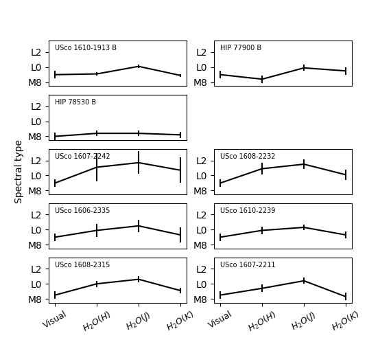
Appendix B shows the systematic differences between each method. The spectral type derived from the H2O index seems to be 1-2 subtype over the one from the visual method. Allers & Liu 2013 explain that the H2O index could be sensitive to gravity and so can be biased. We choose the spectral type from the visual comparison to avoid this bias.
In addition to the spectral-type determination, we also applied the surface gravity classification formalized by Allers & Liu 2013. The results are reported in Table 3 and show that HIP 77900 B and HIP 78530 B are identified as young, intermediate surface gravity BDs. USco 1610-1913 B is confirmed as a very-low surface gravity BD. The gravity class of HIP 78530 B is consistent with the one derived by Lachapelle et al. 2015. Our results are consistent with those of Lodieu et al. 2018 for the classification of the young free-floating objects.
4.1.3 Over-luminosity of USco 1610-1913 B
Figure 5 shows the comparison between the visible and near-infrared calibrated flux of USco 1610-1913 B with the fluxes of young reference BDs of similar spectral types from our sample with Gaia parallaxes. We also include a comparison to the X-Shooter spectrum of TWA 26 (Manara et al. 2013). All BDs have been scaled to the distance of USco 1610-1913A. All these objects reproduce the detailed absorptions and pseudo-continuum shape of USco 1610-1913 B spectrum provided that an extra scaling factor of 2 (TWA 26) and 4 (USco 1610-2239, HIP 77900 B) is considered. This over-luminosity of USco 1610-1913 B had already been noted by Aller et al. 2013 and Lachapelle et al. 2015. We confirm it over our extended wavelength range and resolution relying on an extended set of comparison objects from the association with now published parallaxes. We discuss the possible origins of the over-luminosity in Section 6.
| Spectral Types | Gravity | ||||||||
| Source | Visual | NIR | Scorec | Type | |||||
| H2O (H)a | H2O-1 (J)b | H2O-2 (K)b | FeHz | FeHj | K Ij | H-cont | |||
| USco 1610-1913 B | M9 0.5 | M9.1 0.2 | L0.1 0.2 | M8.9 0.2 | 2 | 2 | 2 | 2 | v-low |
| HIP 77900 B | M9 0.5 | M8.4 0.5 | M9.9 0.4 | M9.5 0.5 | 1 | 2 | 1 | 2 | int |
| HIP 78530 B | M8 0.5 | M8.4 0.4 | M8.4 0.4 | M8.2 0.4 | 1 | 2 | 1 | 2 | int |
| USco 1607-2242 | M9 0.5 | L1.1 1.9 | L1.7 1.5 | L0.7 1.7 | n | 1 | 2 | 2 | v-low |
| USco 1608-2232 | M9 0.5 | L0.9 0.8 | L1.5 0.6 | L0.1 0.7 | 2 | 2 | 1 | 2 | v-low |
| USco 1606-2335 | M9 0.5 | M9.9 0.9 | L0.5 0.8 | M9.3 1.0 | 2 | 1 | 1 | 2 | int |
| USco 1610-2239 | M9 0.5 | M9.9 0.5 | L0.3 0.4 | M9.3 0.5 | 2 | 2 | 2 | 2 | v-low |
| USco 1608-2315 | M8.5 1.0 | L0.0 0.4 | L0.6 0.4 | M9.1 0.4 | 2 | 2 | 1 | 2 | v-low |
| USco 1607-2211 | M8.5 1.0 | M9.4 0.5 | L0.4 0.4 | M8.3 0.5 | 2 | 2 | 1 | 2 | v-low |
- •
Notes: relations and coefficients : [a] From Allers et al. 2007, [b] From Slesnick et al. 2004, and [c] See Allers & Liu 2013. The systematic differences about the spectral type determination are discussed in Appendix B.
4.2 Forward modelling analysis
4.2.1 Description of the atmospheric models
We used a forward-modeling approach to determine the atmospheric parameters of the young BDs observed in this study. Forward modelling codes enable comparison of the object spectrum to pre-computed grids of models which include our best knowledge of atmospheric physics. We used grids of synthetic spectra produced by the BT-SETTL15 model (Allard et al. 2012). This model handles the radiative transfer using the PHOENIX code (Hauschildt et al. 1997; Allard et al. 2001). It accounts for convection using the mixing-length theory, and works at hydrostatic and chemical equilibrium. The opacities are treated line by line (details on each elements are given in Rajpurohit et al. 2018). The code models the condensation, coalescence, and mixing of 55 types of grains. The abundances of solids are determined comparing the timescales of these different processes at each layer. In this study, we considered the predictions of the BT-SETTL15 model with ranging from 2100 K to 3000 K (in steps of 100 K), and a range of log(g) from 3.5 to 5.5 dex (in steps of 0.5 dex). We assumed a solar metallicity M/H = 0.0, in broad agreement with the values reported in Sco-Cen (Bubar et al. 2011). These grids have been extensively utilized in previous studies of young BDs (Manjavacas et al. 2014; Bonnefoy et al. 2014; Delorme et al. 2017b; Bayo et al. 2017), but never as part of a Bayesian methodology, as developed here with the ForMoSA code.

4.2.2 The ForMoSA code
For this work, we chose to develop our own forward modelling code relying on the Nested Sampling procedure (Skilling 2006). The method explores and recursively isolates different patches of likelihood levels in the parameter space. It offers several advantages over classical Markov-Chain-Monte-Carlo algorithms also used for the forward modelling (e.g. Bonnefoy et al. 2018; Samland et al. 2017). The approach avoids missing local minimum within vast and degenerate parameter spaces while ensuring the convergence of the exploration.
The code ForMoSA (for FORward MOdeling for Spectral Analysis) takes as input an observed spectrum with associated error bars and any grid of synthetic spectra (here the BT-SETTL15 grid). The Nested Sampling is handled by the nestle Python module33 3 http://kylebarbary.com/nestle/. ForMoSA re-samples the data and the models to make them comparable. The grid of model spectra are first interpolated onto the wavelength grid of the observation and degraded to the spectral resolution of the instrument that acquired the data. The optical spectra of our targets and the models were degraded to R and , similar to the UVB, VIS and NIR part of the spectrum respectively.
In our case, we suppose independent data points in the observed spectra, so the likelihood is derived from the value. To compute at each step, we need to generate a model spectrum for a set of free-parameters that does not necessarily exist in the original grid of spectra. Therefore, we generated a model spectrum on-demand following a two-step process:
- •
A preliminary phase consists in reducing the grid meshes. To do so, ForMoSA interpolates and reduces each increment to 10 K and log(g) increments to 0.01 dex. We have considered the linear and bicubic spline interpolation approaches, and finally selected the bicubic spline interpolation which better accounts for the flux variation through the grid. This step needs to be done one time and ensure a regular grid. In doing this, we increase the accuracy of the second interpolation phase.
- •
The second phase arises in the course of the Nested Sampling process when a new point in the parameter space is defined. The closest neighbours approach was found to provide the best trade-off between the reliability of the interpolation process and the computation time needed to run the interpolation.
Each synthetic spectrum gives the flux at the top of the atmosphere. The comparison with the observed spectrum requires in addition multiplying the model by a dilution factor , with R the object radius and d the distance. We adopt distances for the host stars from the Gaia DR2. We considered flat priors on (2100-2900 K) and log(g) (3.5-5.5 dex). and radius are linked together by the luminosity (Boltzmann law) so we have chosen a flat prior on R (0.5-30.0 ) to be conservative and ensure we do not limit the exploration of . We also provide the luminosity from the posterior distributions of and ForMoSA can also consider interstellar extinction () as a free parameter using the extinction law from Fitzpatrick & Massa 2007, the radial velocity (RV) by a Doppler shifting law44 4 function PyAstronomy.pyasl.dopplerShift and the projected rotational velocity v.sin(i) according to the rotational broadening law from Gray’s ”The Observation and Analysis of Stellar Photospheres”55 5 function PyAstronomy.pyasl.rotBroad. Figure 6 illustrates a typical output of ForMoSA on HIP 78530 B. The method allows us to identify correlations between parameters such as and R.

4.3 Results
| R | log(g) | ||||
|---|---|---|---|---|---|
| () | (dex) | (K) | Ref | ||
| TWA 26 | a | ||||
| b | |||||
| TWA 29 | a | ||||
| b |
| ForMoSA | Bolometric correction + Evolutionary models | ||||||||
| Object | R | log(g) | R | log(g) | M | ||||
| () | (dex) | (K) | () | (dex) | (K) | () | |||
| USco 1610-1913 B 11footnotemark: 1 | |||||||||
| HIP 77900 B 11footnotemark: 1 | |||||||||
| HIP 78530 B 11footnotemark: 1 | |||||||||
| USco 1607-2242 | |||||||||
| USco 1608-2232 | |||||||||
| USco 1606-2335 | |||||||||
| USco 1610-2239 | |||||||||
| USco 1608-2315 | |||||||||
| USco 1607-2211 | |||||||||
- 1
With the hypothesis that companions are at the same distance than the primary star.
As a safety check, the ForMoSA code was applied to our three companions HIP 78530 B, HIP 77900 B, and USco 1610-1913 B and two well known young BDs, TWA 26 and TWA 29, with similar spectral types and ages (Myr) and observed by Manara et al. 2013. We considered wavelengths from 1.0 to 2.5 in all our fits to avoid biases related to the residual contamination of HIP 78530 B and run a homogeneous analysis on all objects. The results are shown in Figures 7 - 11. The numerical values are given in Tables 6 - 7.
- •
Panels (a), (b), (c) and (d) of Figures 7 - 11 show the X-Shooter spectra (black) with the resulting best fit (blue) considering different spectral windows (, , and , respectively), and a fixed-extinction assumption from the Gaia DR2 extinction maps and values at the location of our targets (Lallement et al. 2019). From these maps, we calculate the extinction at 550.0 nm and assume that the difference with the extinction is negligible ( ). The fitting spectral range is indicated by the yellow background.
- •
Panel (e) shows the best fit when using the complete -band spectral range, and adding the extinction value this time as a free parameter. We reddened the models with an extinction function in the code (Fitzpatrick & Massa 2007).
- •
Panel (f) shows the best fit focused on the optical part (0.56-1.00 for all targets but 0.80-1.00 for HIP 78530 B). We estimate the pseudo-continuum from the original X-Shooter spectrum by degrading it to a very low spectral resolution (), then subtract this pseudo-continuum from the original section to highlight line features. We add the v.sin(i) as a free-parameter with this fit. We determine the radius analytically with the relation from Cushing et al. 2008.
- •
Panel (g) shows of zoomed view on a the gravity/metallicity-sensitive lines of K I and Na I with the best fitting solution. We subtracted the pseudo-continuum in using the same method that in the panel (f). The determination of the radius is analytic too.
Generally, the results show that the BT-SETTL15 models fail to consistently reproduce the pseudo-continuum of the X-Shooter spectra of all objects at all wavelengths (visible and near-infrared) with the same range of physical parameters. The same problem arises when considering a test on the original grid of BT-SETTL15 spectra. This is highlighted in panels (a)-(d) of all figures, where the best fit solution varies considerably depending on which spectral range is fit. Similar discrepancies were evidenced by Manjavacas et al. 2014 using older releases of the models (Allard et al. 2011; Allard et al. 2013; Lachapelle et al. 2015; Bayo et al. 2017; Allard et al. 2012). Therefore, the problem remains in the 2015 release of the models.
The posteriors of are strongly tied to the pseudo-continuum shape. Consequently, they are affected by the choice of the spectral range chosen to estimate the best fit. For instance, the is generally higher from a fit using the J-band compared to fit using H or K-band. The surface gravity is also affected as it remains sensitive to the shape of the VO and H2O absorption bands. Notably, the radius, which is linked to the flux dilution factor, seems to be mostly consistent when using three different fitting bands. In addition to the best fitting solution, the ForMoSA code provides the errors on the posterior solutions. The errors on the posterior solutions are tightly connected to the errors bars on the spectra themselves by the likelihood function. Given the high-S/N of the X-Shooter spectra for HIP 78530 B, HIP 77900 B, USco 1610-1913 B, TWA 26 and TWA 29, the resulting fitting error bars are about one to two orders of magnitude smaller than the systematics associated with the choice of the spectral fitting window, and the non-perfect match of the BT-SETTL15 models with our spectra at all observed wavelengths (see Table 6 - 7). Our adopted solutions in , log(g) and R are therefore derived from the average and dispersion of the solutions from the different spectral fitting windows with the extinction value given by Lallement et al. 2019. The bolometric luminosity is calculated with the Stefan-Boltzmann law.
In addition to different spectral fitting window, the ForMoSA code was also applied with the extinction as a free parameter. The resulting posteriors can be directly compared with the ones obtained with the Gaia DR2 values at the location of our targets (Lallement et al. 2019). Surprisingly, with the simple use of an interstellar extinction law correction, we considerably improve the goodness of the fits of all targets (see Figures 7 - 11 panel (e)). Considering that our targets have no extinction (both sources are located at less than 80 pc; TWA 26 has a transition disk around it but the flux excess appears at , Riaz & Gizis 2008; TWA 29 has no known disk, Rodriguez et al. 2015) or precisely known and low interstellar extinction values ( for our three Upper Sco companions), the excellent good fit of all objects with artificial values of 1.76-2.58 mag indicates a missing physical component in the models. As all objects are affected, it is very likely that the origin is not circumstellar, but linked to the current state of art of BT-SETTL15 models as for example the complexity of the dust formation process or the dust opacity (Pavlenko et al. 2007). Systematically testing how this deficiency evolves with lower effective temperature, age (surface gravity) and gravity would be very interesting.
As an additional step to exploit the medium resolution of our X-Shooter spectra, the radial and rotational velocity information (line profile and offset) has been incorporated into ForMoSA as additional fitting parameters. The radial velocity (RV) can be adjusted on the full spectral window. For the adjustment of v.sin(i), we restricted the fitting window to the optical part (0.56-1.00) with the continuum subtracted to minimize the computation time. This choice is driven by the higher spectral resolution in optical (R = 5400) and the presence of various absorption lines (NaI, FeH or VO). In Table 6 - 7, one can see that the RV results strongly depends on the choice of the fitting spectral window. We adopted the RV value from the optical fit for the same reasons that for the v.sin(i). The two identified causes of this discrepancy are the slope issues in models and a systematic error in the wavelength calibration of the spectra. We therefore decided to independently compute the RVs using a cross-correlation approach between our observed spectra and a spectral template generated by the BT-SETTL15 code at a = 2400K and a log(g) = 4.0 dex (see Figure 12). For most cases, there is a good agreement between the cross-correlation results and the ForMoSA ones in the optical that we therefore adopt as final values. For the rotational velocity, the limited X-Shooter spectral resolution does not allow to measure the low v.sin(i) of our targets, but rahter places an upper limit of roughly 50 km/s. This limit is consistent with the 55 km/s limit expected for a resolution of about R = 5400 in the visible arm. Considering the adopted values of , log(g), R, RV, v.sin(i) and L using the fixed extinction values of Lallement et al. 2019, we now detail the results of ForMoSA target by target.
TWA 26 and TWA 29 : Both targets are well known and their X-Shooter spectra have been analyzed as a sanity check of the ForMoSA code. They have been classified by Manara et al. 2015 as late-M dwarfs with spectral types M and M9.5, respectively. Both are members of the TW Hydrae association, with an age estimate of 8 Myr, and are located at a distance of 49 pc and 83 pc, respectively. They have no extinction observed in their line of sight. Both have been characterized by Filippazzo et al. 2015 using a complimentary approach to our work. Exploiting the spectral energy distribution from the visible to the near-infrared and the mid-infrared, Filippazzo et al. 2015 derived the bolometric luminosities of these two young brown dwarfs with known distances. Using evolutionary model predictions from solar metallicity SMHC08 (Saumon & Marley 2008) and DMESTAR (Feiden & Chaboyer 2012, Feiden & Chaboyer 2013) isochrones, they derived the predicted radii and masses, and therefore the object effective temperatures using the Stefan-Boltzmann law as well as the surface gravities. The results are reported in Table 4, and roughly agree within the error bars with the ones obtained by the ForMoSA forward modelling of the X-Shooter spectra of TWA 26 and TWA 29. As the three Upper Sco companions HIP 78530 B, HIP 77900 B, USco 1610-1913 B scan similar range of temperature and surface gravities than TWA 26 and TWA 29, this test tend to support the use of ForMoSA to explore their physical properties. These three companions have no known mid-infrared photometry or spectroscopy, therefore a direct determination of the bolometric luminosity as done by Filippazzo et al. 2015 is here not possible Based on a fit in using the optic wavelength range, we derive a v.sin(i) km/s for TWA 29. It is only object for which we are not limited by the resolving power of the instrument.
USco 1610-1913 B : For their study of this companion, Lachapelle et al. 2015 used an incorrect value of = 1.1 given by Carpenter et al. 2009. Using the method described in Carpenter et al. 2008, Carpenter et al. 2009 derived this relatively high using the optical (Johnson and , Tycho and ) and near-infrared (2MASS , , and ) photometry and colors, but a wrong spectral type (K7) for USco 1610-1913. As described in Appendix A, an updated analysis of the full SED actually indicates a later spectral type M0, leading to an extinction value of A mag, which is more consistent with the value from Lallement et al. 2019 : = 0.13. Using = 0.13, we derive with ForMoSA an effective temperature of K, a surface gravity of dex, both compatible with a young M9 brown dwarf of very low gravity for USco 1610-1913 B. However, we find clear non-physical solutions for the radius and the luminosity (for a young late-M dwarf), which confirm the strong over-luminosity of this source, as already pointed out in Section 4.1 and that we will discuss further in Section 6. We notice a difference between the radial velocity found from ForMoSA and the one found from the cross-correlation algorithm.
HIP 78530 B : The extinction maps of Lallement et al. 2019 gives a value of = 0.075 along the line of sight of HIP 78530, somewhat different from the value of = 0.5 used by Lachapelle et al. 2015 and from Carpenter et al. 2009. We adopted the former value in our analysis. ForMoSA finds K, in agreement with the M8 spectral type of the source (Luhman et al. 2003; Filippazzo et al. 2015, this work). The analysis of the continuum-subtracted spectrum yields a surface gravity estimate compatible with the intermediate gravity class of the object (Section 4.1). The luminosity value of = is also compatible with expected = -2.5 to -3.0 found by Filippazzo et al. 2015 for young M and M8 BDs. Finally, the effective temperature and surface gravity are consistent with the values from Lafrenière et al. 2011.
HIP 77900 B : With an extinction value of = 0.07 (Lallement et al. 2019), the resulting effective temperature of K given by ForMoSA is consistent with the later M spectral type empirically derived for this companion. The estimated surface gravity of is consistent with the intermediate gravity classification of Allers & Liu 2013, and the luminosity value of = is compatible with the values found for young M9 brown dwarfs (Filippazzo et al. 2015).
| TWA 26 | J | H | K | JHK | JHK and Av | JHK-cont | OPT-cont | OPT-croscor | Adopted |
| (K) | - | a | |||||||
| log(g) (dex) | 3.5 | 3.5 | 3.5 | 3.5 | - | b | |||
| R () | - | a | |||||||
| RV (km/s) | - | ||||||||
| - | c | ||||||||
| (mag) | 0.0 | 0.0 | - | 0.0 d | |||||
| v.sin(i) (km/s) | - | - | |||||||
| TWA 29 | J | H | K | JHK | JHK and Av | JHK-cont | OPT-cont | OPT-croscor | Adopted |
| (K) | - | ||||||||
| log(g) (dex) | 3.5 | 3.5 | 3.5 | - | |||||
| R () | - | ||||||||
| RV (km/s) | - | ||||||||
| - | |||||||||
| 0.0 | 0.0 | - | 0.0 | ||||||
| v.sin(i) (km/s) | - | - | |||||||
| USco 1610-1913 B | J | H | K | JHK | JHK and Av | JHK-cont | OPT-cont | OPT-croscor | Adopted |
| (K) | 2100 | - | |||||||
| log(g) (dex) | 3.5 | 3.5 | - | ||||||
| R () | - | ||||||||
| RV (km/s) | |||||||||
| - | |||||||||
| 0.13 | 0.13 | - | 0.13 | ||||||
| v.sin(i) (km/s) | - | - | |||||||
| HIP 78530 B | J | H | K | JHK | JHK and Av | JHK-cont | OPT-cont | OPT-croscor | Adopted |
| (K) | - | ||||||||
| log(g) (dex) | - | ||||||||
| R () | - | ||||||||
| RV (km/s) | |||||||||
| - | |||||||||
| 0.075 | 0.075 | - | 0.075 | ||||||
| v.sin(i) (km/s) | - | - | |||||||
| HIP 77900 B | J | H | K | JHK | JHK and Av | JHK-cont | OPT-cont | OPT-croscor | Adopted |
| (K) | - | ||||||||
| log(g) (dex) | - | ||||||||
| R () | - | ||||||||
| RV (km/s) | |||||||||
| - | |||||||||
| 0.07 | 0.07 | - | 0.07 | ||||||
| v.sin(i) (km/s) | - | - | |||||||
- •
a Mean and standard deviation between , and bands.
- •
b High value between , , and -cont bands.
- •
c StefanBoltzmann law in using and radius ranges.
- •
d From Lallement et al. 2019’s maps (derived from Galli et al. 2018).
| USco 1606-2335 | J | H | K | JHK | JHK and Av | JHK-cont | OPT-cont | OPT-croscor | Adopted |
| (K) | - | ||||||||
| log(g) (dex) | 3.5 | 3.5 | 3.5 | 5.0 | - | ||||
| R () | - | ||||||||
| RV (km/s) | |||||||||
| - | |||||||||
| (mag) | 0.0 | 0.0 | - | 0.0 d | |||||
| v.sin(i) (km/s) | - | - | |||||||
| USco 1607-2211 | J | H | K | JHK | JHK and Av | JHK-cont | OPT-cont | OPT-croscor | Adopted |
| (K) | - | ||||||||
| log(g) (dex) | 3.5 | 3.5 | - | ||||||
| R () | - | ||||||||
| RV (km/s) | |||||||||
| - | |||||||||
| 0.0 | 0.0 | - | 0.0 | ||||||
| v.sin(i) (km/s) | - | - | |||||||
| USco 1607-2242 | J | H | K | JHK | JHK and Av | JHK-cont | OPT-cont | OPT-croscor | Adopted |
| (K) | 2100 | - | |||||||
| log(g) (dex) | 3.5 | 3.5 | 3.5 | 3.5 | - | ||||
| R () | - | ||||||||
| RV (km/s) | |||||||||
| - | |||||||||
| 0.0 | 0.0 | - | 0.0 | ||||||
| v.sin(i) (km/s) | - | - | |||||||
| USco 1608-2232 | J | H | K | JHK | JHK and Av | JHK-cont | OPT-cont | OPT-croscor | Adopted |
| (K) | 2100 | - | |||||||
| log(g) (dex) | 3.5 | 3.5 | 3.5 | 3.5 | 5.0 | - | |||
| R () | - | ||||||||
| RV (km/s) | |||||||||
| - | |||||||||
| 0.0 | 0.0 | - | 0.0 | ||||||
| v.sin(i) (km/s) | - | - | |||||||
| USco 1608-2315 | J | H | K | JHK | JHK and Av | JHK-cont | OPT-cont | OPT-croscor | Adopted |
| (K) | 2100 | - | |||||||
| log(g) (dex) | 3.5 | 3.5 | 3.5 | - | |||||
| R () | - | ||||||||
| RV (km/s) | |||||||||
| - | |||||||||
| 0.0 | 0.0 | - | 0.0 | ||||||
| v.sin(i) (km/s) | - | - | |||||||
| USco 1610-2239 | J | H | K | JHK | JHK and Av | JHK-cont | OPT-cont | OPT-croscor | Adopted |
| (K) | - | ||||||||
| log(g) (dex) | 3.5 | 3.5 | 3.5 | 3.5 | - | ||||
| R () | - | ||||||||
| RV (km/s) | |||||||||
| - | |||||||||
| 0.0 | 0.0 | - | 0.0 | ||||||
| v.sin(i) (km/s) | - | - | |||||||
5 Emission line properties
Our new high S/N medium-resolution optical spectra allow us to identify the faint (656.28 nm) emission lines of the three companions and of four out of the six free-floating objects of our sample. Figure 14 shows the line profiles at each epoch. We checked for the emission line detection in the traces to ensure it was not produced by an uncorrected bad pixel (see Section 3). lines are commonly attributed to magnetospheric accretion (Manara et al. 2013; Manara et al. 2015; Natta et al. 2004) or chromospheric activity (White & Basri 2003, e.g.,). The three objects (USco 1610-1913 B, USco 1606-2335, and USco 1608-2315) showing the strongest lines also display other Balmer lines, (486.1 nm) and (434.0 nm), in their spectra. We tentatively identify Ca II-H (393.4 nm) and Ca II-K (396.9 nm) emission lines in the spectrum of USco 1610-1913 B as well. The Ca II lines can also be related to accretion or activity (Herczeg & Hillenbrand 2008). We report the apparent fluxes of these emission lines and 10% width of line in Table 8. The noisy spectral continua of our objects prevented us from obtaining robust determination of the continuum and the equivalent widths. Both origins (accretion and activity) for our targets are investigated below.
5.1 Accretion rate determination
The accretion rates of each object are reported in Table 10. They were derived following the relation of Alcalá et al. 2017:
| (1) |
where is the accretion luminosity, is the inner disk radius, and are the radius and mass of the objects, respectively. This is assuming / = 0.2 (Alcalá et al. 2017) which holds in our mass range and whatever the object configuration (companion or isolated). The accretion luminosities were estimated beforehand from the line fluxes of the Ca II lines and the Balmer lines using the relationships given in Rigliaco et al. 2012 and Alcalá et al. 2017, respectively. Radii and masses were in addition inferred from the evolutionary model predictions as indicated in Table 5.
Alternatively, we derived accretion rates based on 10% width following the relations of Natta et al. 2004:
| (2) |
The 10% accretion rates are also reported in Table 10. They tend to be higher than the ones inferred from the Balmer and Ca II line fluxes. A similar divergence between the different accretion proxies is found for the young companion SR 12C (Santamaría-Miranda et al. 2018). The accretion rates of USco 1610-1913 B are compatible with those of the 1-5 Myr late-M sub-stellar companions FW Tau b (Bowler et al. 2014), DH Tau b (Zhou et al. 2014), and GQ Lup b (Wu et al. 2017b), which had the lowest recorded accretion rates among known accreting companions. The accretion rates of HIP 78530 B and HIP 77900 B are found to be an order of magnitude lower, this indicates these objects as non-accretor.
5.2 Chromospheric activity
The weakness of the lines suggests the emission arises mostly from chromospheric activity. Manara et al. 2013 provides the values expected from chromospheric activity for young stars and brown-dwarfs, down to the M9 spectral type:
| (3) |
All our objects but USco 1608-2315 have values below or comparable to the activity threshold corresponding to their (estimated from ForMoSA), thus indicating that the lines are indeed likely related to chromospheric activity. Herczeg et al. 2009 also identify a line on USco 1607-2211 of similar intensity and reach the same conclusion. We note that this criterion applied to the line of GQ Lup b as observed on 2015, April 2016 (Wu et al. 2017b) indicates that the line mostly arises from chromospheric activity in spite of accretion at this epoch77 7 We considered the from Seifahrt et al. 2007 and Zhou et al. 2014 and the luminosity from Zhou et al. 2014 to compute the = -3.8 to -3.48 value and compare it to of the object.. The 10% width of the line may also discriminate between the accretion (large values) and chromospheric activity (small values). A threshold of 200 km.s-1 is generally adopted for brown-dwarfs (Jayawardhana et al. 2003). All of our objects but USco 1608-2315 have an 10% below the 200 km.s-1 limit, thus supporting line production by chromospheric activity. Therefore, USco 1608-2315 is likely the only true accreting object in our sample. The source also has a tentative disk excess (Section 2). Thus, we add USco 1608-2315 to the short list of free-floating accretors with masses below 30 (Herczeg et al. 2009; Bayo et al. 2012; Joergens et al. 2013; Alcalá et al. 2014; Boucher et al. 2016; Lodieu et al. 2018).
To further support these conclusions for a few specific objects, Figure 13 compares the UVB spectra of USco 1610-1913 B and TWA 26 scaled to the distance of USco 1610-1913 B. The flux from TWA 26 had to be multiplied by an additional factor of two to match USco 1610-1913 B’s flux level (see Section 6.2). The pseudo-continuum of USco 1610-1913 B is well reproduced by a template with emission lines due to chromospheric activity (Manara et al. 2013). The and lines have similar strengths but the line appears more luminous in the companion spectrum.
Figure 14 shows that the two free-floating objects with the strongest lines (USco 1608-2315 and USco 1606-2335) display significant short-term variability. The lines are not detected in the optical spectra of these objects obtained in May 2007 (Lodieu et al. 2011). The lines of USco 1607-2211 and USco 1610-2239 do not show obvious variability in our data, but are not detected in May 2007 (Lodieu et al. 2011) as well. It is possible that the non-detections from 2007 arise from a degraded sensitivity of the low resolution data from Lodieu et al. 2011. Active M-dwarfs are known to display such variability from chromospheric activity (Gizis et al. 2002, e.g.,), which strengthens our conclusions on the line origins. The variability of USco 1608-2315 could also stem from variation of the accretion rate (Aguayo et al., in prep; Bonnefoy et al., in prep.).
| Object | Date | Ca II-H | Ca II-K | 10% | |||
| () | () | () | () | () | () | ||
| USco 1610-1913 B | 2014-04-02 | 145 | |||||
| HIP 77900 B | 2014-04-12 05:45UT | … | |||||
| HIP 77900 B | 2014-04-12 08:38UT | … | |||||
| HIP 78530 B | 2014-06-09 04:08UT | … | |||||
| HIP 78530 B | 2014-06-09 05:14UT | … | |||||
| USco 1607-2242 | all epochs | … | |||||
| USco 1608-2232 | all epochs | … | |||||
| USco 1606-2335 | 2014-06-25 | … | |||||
| USco 1606-2335 | 2014-06-30 | 169 | |||||
| USco 1606-2335 | 2014-07-04 | 136 | |||||
| USco 1606-2335 | 2014-07-29 | 105: | |||||
| USco 1610-2239 | 2014-06-30 | … | |||||
| USco 1610-2239 | 2014-07-01 03:26UT | … | |||||
| USco 1610-2239 | 2014-07-01 04:04UT | … | |||||
| USco 1608-2315 | 2014-06-15 | 220 | |||||
| USco 1608-2315 | 2014-06-20 | 209 | |||||
| USco 1607-2211 | 2014-04-22 | 160 | |||||
| USco 1607-2211 | 2014-06-14 | … | … |
| Object | Date | Ca II-H | Ca II-K | Balmer | ||||
|---|---|---|---|---|---|---|---|---|
| USco 1610-1913 B | 2014-04-02 | |||||||
| HIP 77900 B | 2014-04-12 05:45UT | |||||||
| HIP 77900 B | 2014-04-12 08:38UT | |||||||
| HIP 78530 B | 2014-06-09 04:08UT | |||||||
| HIP 78530 B | 2014-06-09 05:14UT | |||||||
| USco 1607-2242 | all epochs | … | … | |||||
| USco 1608-2232 | all epochs | … | … | |||||
| USco 1606-2335 | 2014-06-25 | |||||||
| USco 1606-2335 | 2014-06-30 | |||||||
| USco 1606-2335 | 2014-07-04 | |||||||
| USco 1606-2335 | 2014-07-29 | |||||||
| USco 1610-2239 | 2014-06-30 | |||||||
| USco 1610-2239 | 2014-07-01 03:26UT | |||||||
| USco 1610-2239 | 2014-07-01 04:04UT | |||||||
| USco 1608-2315 | 2014-06-15 | |||||||
| USco 1608-2315 | 2014-06-20 | |||||||
| USco 1607-2211 | 2014-04-22 | |||||||
| USco 1607-2211 | 2014-06-14 | … | … | … |
| Object | Date | Ca II-H | Ca II-K | 10% | |||
|---|---|---|---|---|---|---|---|
| log(/year) | log(/year) | log(/year) | log(/year) | log(/year) | log(/year) | ||
| USco 1610-1913 B | 2014-04-02 | ||||||
| HIP 77900 B | 2014-04-12 05:45UT | … | |||||
| HIP 77900 B | 2014-04-12 08:38UT | … | |||||
| HIP 78530 B | 2014-06-09 04:08UT | … | |||||
| HIP 78530 B | 2014-06-09 05:14UT | … | |||||
| USco 1607-2242 | all epochs | … | |||||
| USco 1608-2232 | all epochs | … | |||||
| USco 1606-2335 | 2014-06-25 | … | |||||
| USco 1606-2335 | 2014-06-30 | ||||||
| USco 1606-2335 | 2014-07-04 | ||||||
| USco 1606-2335 | 2014-07-29 | ||||||
| USco 1610-2239 | 2014-06-30 | … | |||||
| USco 1610-2239 | 2014-07-01 03:26UT | … | |||||
| USco 1610-2239 | 2014-07-01 04:04UT | … | |||||
| USco 1608-2315 | 2014-06-15 | ||||||
| USco 1608-2315 | 2014-06-20 | ||||||
| USco 1607-2211 | 2014-04-22 | ||||||
| USco 1607-2211 | 2014-06-14 | … | … |
6 Discussion
6.1 Revisiting the physical association of HIP 77900 B and USco 1610-1913 B with Gaia
HIP 77900 B and USco 1610-1913 B are bright enough and distant enough from their primary so that they have reported Gaia parallaxes. This is to our knowledge the first case for which the physical association of young imaged BD companions with their primary stars can be investigated based on the individual 5-parameters astrometric solutions of the system components.
6.1.1 The case of HIP 77900 B
The Gaia-DR2 parallax of HIP 77900 A confirms that the system would be extreme if bound (au projected separation). Very wide systems such as HIP 77900 are expected to be rare (Baron et al. 2018, e.g., ). The companion has not been observed at multiple epochs so it could in principle be a background star. However, the close resemblance of the companion’s spectrum to those of free-floating analogues from our library of Upper-Sco objects identifies it as a likely member of this association. Therefore, HIP 77900 A and B are either coeval or aligned by chance within the association. Their respective distances ( pc for A, and pc for B) reveal a 1.4 difference. There is in addition a 1.8 difference between the proper motion in declination of the two objects. The p-value on the difference on the 3 astrometric parameters of A and B (0.06) does not allow us to firmly conclude whether the system is coeval. The RUWE values of A and B (0.97 and 1.21) indicate robust solutions. The galactic Cartesian coordinates of HIP 77900 A ( pc, pc, pc) computed following Gagné et al. 2014 are well within the range of expected values for Upper-Sco (Galli et al. 2018), contrary to the ones of B ( pc, pc, pc) which is at odds with the youth of the object. However, we find photometric distances of pc and pc for HIP 77900 B using the flux-calibrated spectra of the spectral analogue M8.5 dwarfs from our sample (USco 1607-2211 and USco 1610-2239, respectively) with Gaia parallaxes. These photometric distances are more consistent with the Gaia distance of A and would strengthen the case of a coeval system. However, we found a RV of km/s for the B component not consistent with the km/s found by Gontcharov 2006 for HIP 77900 A. This result raises severe doubts about the gravitational link between both objects, and the next Gaia data releases of the relative astrometry of A and B will be needed to firmly conclude on the physical association of both objects.
6.1.2 The case of USco 1610-1913 B
The spectral properties and measured distance of USco 1610-1913 B clearly confirm its membership to Upper-Sco. The two objects have been shown to have a common proper motion from 2007 to 2012 and have been proposed to be bound (Kraus et al. 2014, and ref therein). However, the recent DR2 solutions of USco 1610-1913 B and A diverge in proper motion (2.0 and 2.4 significance in and , respectively) and in distance (1.4 ; B is 10.3 pc closer than A). A test on the difference on the 3 astrometric parameters of each system component (parallaxes and proper motions) taking into account the correlations, gives a p-value of 0.01 which is in favor of a physical bond between both objects. The p-value accounts for the slight under-estimation of the errors (Lindegren et al. 2018). The reliability of the Gaia astrometry may however be questioned for this particular system. Indeed, the M-dwarf companion to USco 1610-1913 A (Kraus et al. 2008) is unresolved in the DR2. The Re-normalised Unit Weight Error (RUWE) index is proposed as a reliable and informative goodness-of-fit statistic than for instance the astrometric excess noise (Lindegren et al. 2018, Gaia technical note Gaia-C3-TN-LU-LL-124-01). The RUWE of USco 1610-1913 A (1.63) is above the threshold of 1.4 and indicates that the observations are inconsistent with a simple 5-parameter astrometric model while B (RUWE=1.19) shows a more reliable solution. The next releases of Gaia will here again solve this ambiguity.
If we keep the hypothesis that the system is bound (or even coeval) and located at the distance of the B component, USco 1610-1913 B remains 4.5 times more luminous than free-floating analogues from the Upper Sco association. This is illustrated in Figure 5 using for comparison USco 1607-2211 and USco 1610-2239 which both have high quality astrometric solutions. In addition, the probability for a chance-alignment within the association is slim. Aller et al. 2013 identified USco 1610-1913 B while searching for distant companions within 30 arcseconds from Upper Sco stars and with optical (Pan-Starrs) and near-infrared (UKIDSS) colors compatible with young, cool objects. Using the now available Pan-Starrs data (Chambers et al. 2016), we confirm that USco 1610-1913 B belongs to one of the three objects with the reddest and colors within 5 arcmins of USco 1610-1913 A. It is also the only object in this field with colors typical of M7-M9 Upper-Sco objects. Dahm et al. 2012 determined a RV of km/s for USco 1610-1913 A. USco 1610-1913 B is the unique target for which with find a strong discrepancy between the RV determined by ForMoSA and the cross-correlation approach ( km/s and 0.9 km/s, respectively). Both values are in addition inconsistent with the RV derived by Dahm et al. 2012 for the A component, and therefore inconclusive. Although we cannot firmly exclude that USco 1610-1913 A and B are simply chance aligned members of Upper-Sco, parallaxes and common proper motion do support that they form at least a comoving and possible coeval pair.
6.2 The over-luminosity of USco 1610-1913 B
Evolutionary models of Chabrier et al. 2000 predict a = 2827169 K for USco 1610-1913 B using the bolometric luminosity of the source. This corresponds to a M5 brown dwarf (see Table 5), incompatible with the spectral type of M90.5 derived from our empirical analysis. Our results using the ForMoSA code (see Section 4.3) further confirms this over-luminosity, based on model atmosphere fits. There are several other sources in literature which are similarly over-luminous, such as USco 1602-2401 B (Aller et al. 2013) or 2MASS J162243.85-195105.7 (Dahm et al. 2012). Aller et al. 2013 proposed that differences in the accretion history of USco 1610-1913 B could play a role in such a discrepancy as proposed by Baraffe et al. 2012. For late K and M-dwarfs, chromospheric activity as found in our spectra decreases the objects and increases their radii (López-Morales 2007; Morales et al. 2008). Based on a sample of 669 M non-accreting stars from the Palomar/Michigan State University catalog (PMSU; Reid et al. 1995; Hawley et al. 1996), Stassun et al. 2012 proposed empirical relations to determine the bias induced by chromospheric activity :
| (4) |
| (5) |
Despite this variations of the atmosphere’s radius and , the bolometric luminosity remains constant. This effect can’t explain the over-luminosity of USco 1610-1913 B. An alternative explanation would be that the companion is an unresolved quadruple system presumably with all components having similar spectral types, in this case. Such systems are expected to be rare among A and FG-type stars (Raghavan et al. 2010; De Rosa et al. 2014; Tokovinin 2014). The system would be even more exotic and rare, considering that USco 1610-1913 A is a binary and that USco 1610-1913 B has to be composed by four identical objects to account for its overluminosity. Quadruples tend to be found as 2+2 tight binary systems. The discovery of a quadruple system made of two pairs of M5 eclipsing binaries in Upper-Sco (Wang et al. 2018) show that such object exist in isolation. To our knowledge, adaptive-optics images of the system have not displayed PSF-elongation nor resolved the companion as a higher-order object but new near-infrared high-resolution (R 80 000 to 100 000) spectrographs (ESO/NIRPS, CRIRES+) could investigate the multiplicity of USco 1610-1913B in the near-future.
7 Conclusion
Based on medium resolution spectra obtained with the X-Shooter spectrograph at VLT, we carried out an in-depth characterization of three low-mass brown dwarf companions on wide-orbits, specifically USco 161031.9-16191305 B, HIP 77900 B, and HIP 78530 B of the Upper-Scorpius association, together with six young isolated brown dwarfs of similar spectral types and ages. The X-Shooter data yield the first medium-resolution optical spectra of the companion objects. We can summarize the main results as follow:
- 1.
the re-investigation of the spectral classification of the three companions USco 1610-1913 B, HIP 77900 B and HIP 78530 B confirms that they have spectral types M, M, and M8, respectively. HIP 77900 B and HIP 78530 B are identified as young, intermediate surface gravity brown dwarfs, whereas USco 1610-1913 B is confirmed as a very-low surface gravity brown dwarf.
- 2.
the development and use of the ForMoSA forward modelling code relying on the Nested Sampling procedure enables us to infer posterior probability distributions of the physical properties (, log(g), , and extinction) of USco 1610-1913 B, HIP 77900 B and HIP 78530 B using the BT-SETTL15 atmospheric models and the X-Shooter spectra. We find that generally, the models fail to reproduce the pseudo-continuum of the X-Shooter spectra over broad wavelengths range. Our solutions are mainly affected by the choice of the spectral range considered to estimate the best fit, and the fitting error bars remain about one to two orders of magnitude smaller given the high S/N of the X-Shooter spectra. Finally, when the extinction is considered as a free parameter, the ForMoSA fitting solutions are considerably improved at all wavelengths with extinction values of 1.6-2.6 mag suggesting a clear deficiency in the dust grain modeling of the BT-SETTL15 atmospheric models. These inconsistencies limit our ability to investigate at this stage the chemical abundance of heavy elements in the atmosphere of these young brown dwarfs that could trace different formation mechanisms. Finally, the key physical properties such as , log(g), are in agreement with the empirical analysis, but indicate a clear over-luminosity for USco 1610-1913 B.
- 3.
the study of the medium resolution optical part of the X-Shooter spectra allowed us to identify the presence of various Balmer lines for the three companions USco 1610-1913 B, HIP 77900 B and HIP 78530 B, and the two isolated brown dwarfs USco 1608-2315 and USco 1607-2211, and to investigate their origin. Their low accretion rate, low accretion luminosity and low 10% width tend to support them as signatures tracing chromospheric activity except for USco 1608-2315, which adds to the limited population of accreting free-floating young brown dwarf with mass below 30 .
- 4.
the nature of USco 1610-1913 B and HIP 77900 B is then revisited and discussed in the context of the new Gaia DR2 results. The Gaia solutions of USco 1610-1913 A are probably affected by the binarity of USco 1610-1913 A itself. For HIP 77900 B, the parallax is surprisingly inconsistent with the photometric distance. Nevertheless, a coeval (bound or unbound) configuration remains the most plausible one for both systems. Finally, we showed that the over-luminosity of USco 1610-1913 B cannot be explained by chromospheric activity suggesting that it might be a high-order multiple component if we want to reconcile spectral type and observed luminosity. It calls for further studies using high-resolution spectrographs () like ESO3.6m/NIRPS or VLT/CRIRES+ to explore such an hypothesis.
Acknowledgements.
The authors thank the ESO staff for conducting the observations. We are grateful to D. Lachapelle for providing the spectra of HIP 78530 B and USco 1610-1913 B. We also thank J. Bouvier for advising us on accretion process and chromospheric activity effects. We acknowledge financial support from the Programme National de Planétologie (PNP), the Programme National de Physique Stellaire (PNPS) of CNRS-INSU in France, and the Agence Nationale de la Recherche (GIPSE project; grant ANR-14-CE33-0018). This research has made use of the SIMBAD database and VizieR catalogue access tool (operated at CDS, Strasbourg, France). This research has made use of NASA’s Astrophysics Data System and of the Extrasolar Planet Encyclopedia (http://exoplanet.eu/). This publication makes use of VOSA, developed under the Spanish Virtual Observatory project supported from the Spanish MINECO through grant AyA2017-84089. G-DM acknowledges the support of the DFG priority program SPP 1992 “Exploring the Diversity of Extrasolar Planets” (KU 2849/7-1).Appendix A Temperature and reddenning of USco 1610-1913.
We built the spectral energy distribution (SED) of USco 1610-1913 from SDSS (Alam et al. 2015, u, g, r, i bands), APASS (Henden et al. 2016, B and V bands), Pan-Starrs (Chambers et al. 2016, y band), 2MASS (Cutri et al. 2003, J, H, Ks) and WISE (Cutri & et al. 2013, W1, W2, W3 bands) photometry collected through the VOSA (Bayo et al. 2008) web interface1010 10 http://svo2.cab.inta-csic.es/theory/vosa/index.php supplemented by Spitzer (8, 24) photometry taken from Carpenter et al. 2006.
We compared deredenned SED of the object to synthetic spectra from the BT-NEXTGEN library (Allard et al. 2012) with in the range 3500-4000K and M/H = 0. The surface gravity was varied from 3.0 to 5.0 dex and does not influence the fit. We considered in the range 0-5 mag in steps of 0.01 mag and a reddenning law (Draine 2003a; Draine 2003c; Draine 2003b) with a reddenning parameter .
We find a best fit for = 3800100 K and = 0.090.01 mag) (Fig. 15). The temperature is in broad agreement (Pecaut & Mamajek 2013) with that expected for the quoted K7 spectral type (Preibisch et al. 2001) and rather suggests a M0 type for the object. We confirm the lack of an excess up to 24 . The fit clearly excludes solutions at a higher and a reddenning of = 1.1 mag as reported by Carpenter et al. 2009.
Appendix B Systematic differences in spectral type determination.
To determine the spectral type of our sources we focused on the visible in using a standard comparison between our spectra and the Ultracool RIZzo Spectral Library (see Section 4.1). We also used relations between the spectral type and the H2O absorption bands from Allers et al. 2007 (H2O (H)) and Slesnick et al. 2004 (H2O (J) ; H2O K). Figure 16 shows the systematic differences according to each method used to determine the spectral type.
References
- Alam et al. (2015) Alam, S., Albareti, F. D., Allende Prieto, C., et al. 2015, The Astrophysical Journal Supplement Series, 219, 12
- Alcalá et al. (2017) Alcalá, J. M., Manara, C. F., Natta, A., et al. 2017, A&A, 600, A20
- Alcalá et al. (2014) Alcalá, J. M., Natta, A., Manara, C. F., et al. 2014, A&A, 561, A2
- Allard et al. (2001) Allard, F., Hauschildt, P. H., Alexander, D. R., Tamanai, A., & Schweitzer, A. 2001, ApJ, 556, 357
- Allard et al. (2011) Allard, F., Homeier, D., & Freytag, B. 2011, in Astronomical Society of the Pacific Conference Series, Vol. 448, 16th Cambridge Workshop on Cool Stars, Stellar Systems, and the Sun, ed. C. Johns-Krull, M. K. Browning, & A. A. West, 91
- Allard et al. (2012) Allard, F., Homeier, D., & Freytag, B. 2012, Philosophical Transactions of the Royal Society of London Series A, 370, 2765
- Allard et al. (2013) Allard, F., Homeier, D., Freytag, B., et al. 2013, Memorie della Societa Astronomica Italiana Supplementi, 24, 128
- Aller et al. (2013) Aller, K. M., Kraus, A. L., Liu, M. C., et al. 2013, ApJ, 773, 63
- Allers (2012) Allers, K. N. 2012, in IAU Symposium, Vol. 282, From Interacting Binaries to Exoplanets: Essential Modeling Tools, ed. M. T. Richards & I. Hubeny, 105–110
- Allers et al. (2007) Allers, K. N., Jaffe, D. T., Luhman, K. L., et al. 2007, ApJ, 657, 511
- Allers & Liu (2013) Allers, K. N. & Liu, M. C. 2013, ApJ, 772, 79
- Ardila et al. (2000) Ardila, D., Martín, E., & Basri, G. 2000, AJ, 120, 479
- Baraffe et al. (2003) Baraffe, I., Chabrier, G., Barman, T. S., Allard, F., & Hauschildt, P. H. 2003, A&A, 402, 701
- Baraffe et al. (2015) Baraffe, I., Homeier, D., Allard, F., & Chabrier, G. 2015, A&A, 577, A42
- Baraffe et al. (2012) Baraffe, I., Vorobyov, E., & Chabrier, G. 2012, ApJ, 756, 118
- Barman et al. (2011) Barman, T. S., Macintosh, B., Konopacky, Q. M., & Marois, C. 2011, ApJ, 735, L39
- Baron et al. (2018) Baron, F., Artigau, É., Rameau, J., et al. 2018, ArXiv e-prints, arXiv:1807.08799
- Bate et al. (2002) Bate, M. R., Bonnell, I. A., & Bromm, V. 2002, MNRAS, 332, L65
- Bayo et al. (2017) Bayo, A., Barrado, D., Allard, F., et al. 2017, MNRAS, 465, 760
- Bayo et al. (2012) Bayo, A., Barrado, D., Huélamo, N., et al. 2012, A&A, 547, A80
- Bayo et al. (2008) Bayo, A., Rodrigo, C., Barrado Y Navascués, D., et al. 2008, A&A, 492, 277
- Béjar et al. (2008) Béjar, V. J. S., Zapatero Osorio, M. R., Pérez-Garrido, A., et al. 2008, ApJ, 673, L185
- Biller et al. (2011) Biller, B., Allers, K., Liu, M., Close, L. M., & Dupuy, T. 2011, ApJ, 730, 39
- Bonnefoy et al. (2014) Bonnefoy, M., Chauvin, G., Lagrange, A. M., et al. 2014, A&A, 562, A127
- Bonnefoy et al. (2018) Bonnefoy, M., Perraut, K., Lagrange, A.-M., et al. 2018, A&A, 618, A63
- Boucher et al. (2016) Boucher, A., Lafrenière, D., Gagné, J., et al. 2016, ApJ, 832, 50
- Bowler et al. (2015) Bowler, B. P., Andrews, S. M., Kraus, A. L., et al. 2015, ApJ, 805, L17
- Bowler et al. (2014) Bowler, B. P., Liu, M. C., Kraus, A. L., & Mann, A. W. 2014, ApJ, 784, 65
- Bowler et al. (2011) Bowler, B. P., Liu, M. C., Kraus, A. L., Mann, A. W., & Ireland, M. J. 2011, ApJ, 743, 148
- Bubar et al. (2011) Bubar, E. J., Schaeuble, M., King, J. R., Mamajek, E. E., & Stauffer, J. R. 2011, AJ, 142, 180
- Burrows et al. (1997) Burrows, A., Marley, M., Hubbard, W. B., et al. 1997, ApJ, 491, 856
- Carpenter et al. (2008) Carpenter, J. M., Bouwman, J., Silverstone, M. D., et al. 2008, ApJS, 179, 423
- Carpenter et al. (2006) Carpenter, J. M., Mamajek, E. E., Hillenbrand, L. A., & Meyer, M. R. 2006, ApJ, 651, L49
- Carpenter et al. (2009) Carpenter, J. M., Mamajek, E. E., Hillenbrand, L. A., & Meyer, M. R. 2009, ApJ, 705, 1646
- Chabrier et al. (2000) Chabrier, G., Baraffe, I., Allard, F., & Hauschildt, P. 2000, ApJ, 542, L119
- Chambers et al. (2016) Chambers, K. C., Magnier, E. A., Metcalfe, N., et al. 2016, ArXiv e-prints, arXiv:1612.05560
- Charnay et al. (2018) Charnay, B., Bézard, B., Baudino, J. L., et al. 2018, ApJ, 854, 172
- Cruz et al. (2007) Cruz, K. L., Reid, I. N., Kirkpatrick, J. D., et al. 2007, AJ, 133, 439
- Cruz et al. (2003) Cruz, K. L., Reid, I. N., Liebert, J., Kirkpatrick, J. D., & Lowrance, P. J. 2003, AJ, 126, 2421
- Cushing et al. (2008) Cushing, M. C., Marley, M. S., Saumon, D., et al. 2008, ApJ, 678, 1372
- Cushing et al. (2005) Cushing, M. C., Rayner, J. T., & Vacca, W. D. 2005, ApJ, 623, 1115
- Cutri & et al. (2013) Cutri, R. M. & et al. 2013, VizieR Online Data Catalog, II/328
- Cutri et al. (2003) Cutri, R. M., Skrutskie, M. F., van Dyk, S., et al. 2003, 2MASS All Sky Catalog of point sources.
- Dahm et al. (2012) Dahm, S. E., Slesnick, C. L., & White, R. J. 2012, ApJ, 745, 56
- Dai et al. (2010) Dai, Y., Wilner, D. J., Andrews, S. M., & Ohashi, N. 2010, AJ, 139, 626
- David et al. (2019) David, T. J., Hillenbrand, L. A., Gillen, E., et al. 2019, ApJ, 872, 161
- Dawson et al. (2013) Dawson, P., Scholz, A., Ray, T. P., et al. 2013, MNRAS, 429, 903
- de Bruijne (1999) de Bruijne, J. H. J. 1999, MNRAS, 310, 585
- De Rosa et al. (2014) De Rosa, R. J., Patience, J., Wilson, P. A., et al. 2014, MNRAS, 437, 1216
- de Zeeuw et al. (1999) de Zeeuw, P. T., Hoogerwerf, R., de Bruijne, J. H. J., Brown, A. G. A., & Blaauw, A. 1999, AJ, 117, 354
- Delorme et al. (2017a) Delorme, P., Dupuy, T., Gagné, J., et al. 2017a, A&A, 602, A82
- Delorme et al. (2017b) Delorme, P., Schmidt, T., Bonnefoy, M., et al. 2017b, A&A, 608, A79
- Draine (2003a) Draine, B. T. 2003a, ARA&A, 41, 241
- Draine (2003b) Draine, B. T. 2003b, ApJ, 598, 1017
- Draine (2003c) Draine, B. T. 2003c, ApJ, 598, 1026
- Esplin et al. (2018) Esplin, T. L., Luhman, K. L., Miller, E. B., & Mamajek, E. E. 2018, AJ, 156, 75
- Feiden & Chaboyer (2012) Feiden, G. A. & Chaboyer, B. 2012, ApJ, 761, 30
- Feiden & Chaboyer (2013) Feiden, G. A. & Chaboyer, B. 2013, ApJ, 779, 183
- Filippazzo et al. (2015) Filippazzo, J. C., Rice, E. L., Faherty, J., et al. 2015, ApJ, 810, 158
- Fitzpatrick & Massa (2007) Fitzpatrick, E. L. & Massa, D. 2007, ApJ, 663, 320
- Freudling et al. (2013) Freudling, W., Romaniello, M., Bramich, D. M., et al. 2013, A&A, 559, A96
- Gagné et al. (2014) Gagné, J., Lafrenière, D., Doyon, R., Malo, L., & Artigau, É. 2014, ApJ, 783, 121
- Gagné et al. (2018) Gagné, J., Mamajek, E. E., Malo, L., et al. 2018, ApJ, 856, 23
- Galli et al. (2018) Galli, P. A. B., Joncour, I., & Moraux, E. 2018, MNRAS, 477, L50
- Garrison (1967) Garrison, R. F. 1967, ApJ, 147, 1003
- Gizis et al. (2002) Gizis, J. E., Reid, I. N., & Hawley, S. L. 2002, AJ, 123, 3356
- Gontcharov (2006) Gontcharov, G. A. 2006, Astronomy Letters, 32, 759
- Hauschildt et al. (1997) Hauschildt, P. H., Baron, E., & Allard, F. 1997, ApJ, 483, 390
- Hawley et al. (1996) Hawley, S. L., Gizis, J. E., & Reid, I. N. 1996, AJ, 112, 2799
- Helling & Woitke (2006) Helling, C. & Woitke, P. 2006, A&A, 455, 325
- Henden et al. (2016) Henden, A. A., Templeton, M., Terrell, D., et al. 2016, VizieR Online Data Catalog, II/336
- Herczeg et al. (2009) Herczeg, G. J., Cruz, K. L., & Hillenbrand, L. A. 2009, ApJ, 696, 1589
- Herczeg & Hillenbrand (2008) Herczeg, G. J. & Hillenbrand, L. A. 2008, ApJ, 681, 594
- Hester et al. (1996) Hester, J. J., Scowen, P. A., Sankrit, R., et al. 1996, AJ, 111, 2349
- Houk & Smith-Moore (1988) Houk, N. & Smith-Moore, M. 1988, Michigan Catalogue of Two-dimensional Spectral Types for the HD Stars. Volume 4, Declinations -26.0deg to -12.0deg.
- Ireland et al. (2011) Ireland, M. J., Kraus, A., Martinache, F., Law, N., & Hillenbrand, L. A. 2011, ApJ, 726, 113
- Jayawardhana et al. (2003) Jayawardhana, R., Ardila, D. R., Stelzer, B., & Haisch, Karl E., J. 2003, AJ, 126, 1515
- Joergens et al. (2013) Joergens, V., Bonnefoy, M., Liu, Y., et al. 2013, A&A, 558, L7
- Kausch et al. (2015) Kausch, W., Noll, S., Smette, A., et al. 2015, A&A, 576, A78
- Kirkpatrick (2005) Kirkpatrick, J. D. 2005, ARA&A, 43, 195
- Kirkpatrick et al. (2012) Kirkpatrick, J. D., Gelino, C. R., Cushing, M. C., et al. 2012, ApJ, 753, 156
- Kopytova et al. (2014) Kopytova, T. G., Crossfield, I. J. M., Deacon, N. R., et al. 2014, ApJ, 797, 3
- Kouwenhoven et al. (2005) Kouwenhoven, M. B. N., Brown, A. G. A., Zinnecker, H., Kaper, L., & Portegies Zwart, S. F. 2005, A&A, 430, 137
- Kraus & Hillenbrand (2008) Kraus, A. L. & Hillenbrand, L. A. 2008, ApJ, 686, L111
- Kraus & Hillenbrand (2009) Kraus, A. L. & Hillenbrand, L. A. 2009, ApJ, 703, 1511
- Kraus & Hillenbrand (2012) Kraus, A. L. & Hillenbrand, L. A. 2012, ApJ, 757, 141
- Kraus et al. (2014) Kraus, A. L., Ireland, M. J., Cieza, L. A., et al. 2014, ApJ, 781, 20
- Kraus et al. (2008) Kraus, A. L., Ireland, M. J., Martinache, F., & Lloyd, J. P. 2008, ApJ, 679, 762
- Lachapelle et al. (2015) Lachapelle, F.-R., Lafrenière, D., Gagné, J., et al. 2015, ApJ, 802, 61
- Lafrenière et al. (2011) Lafrenière, D., Jayawardhana, R., Janson, M., et al. 2011, ApJ, 730, 42
- Lafrenière et al. (2008) Lafrenière, D., Jayawardhana, R., & van Kerkwijk, M. H. 2008, ApJ, 689, L153
- Lafrenière et al. (2010) Lafrenière, D., Jayawardhana, R., & van Kerkwijk, M. H. 2010, ApJ, 719, 497
- Lallement et al. (2019) Lallement, R., Babusiaux, C., Vergely, J. L., et al. 2019, arXiv e-prints [arXiv:1902.04116]
- Lindegren et al. (2018) Lindegren, L., Hernández, J., Bombrun, A., et al. 2018, A&A, 616, A2
- Lodieu et al. (2011) Lodieu, N., Dobbie, P. D., & Hambly, N. C. 2011, A&A, 527, A24
- Lodieu et al. (2008) Lodieu, N., Hambly, N. C., Jameson, R. F., & Hodgkin, S. T. 2008, MNRAS, 383, 1385
- Lodieu et al. (2007) Lodieu, N., Hambly, N. C., Jameson, R. F., et al. 2007, MNRAS, 374, 372
- Lodieu et al. (2018) Lodieu, N., Zapatero Osorio, M. R., Béjar, V. J. S., & Peña Ramírez, K. 2018, MNRAS, 473, 2020
- López-Morales (2007) López-Morales, M. 2007, ApJ, 660, 732
- Luhman et al. (2018) Luhman, K. L., Herrmann, K. A., Mamajek, E. E., Esplin, T. L., & Pecaut, M. J. 2018, AJ, 156, 76
- Luhman & Mamajek (2012) Luhman, K. L. & Mamajek, E. E. 2012, ApJ, 758, 31
- Luhman et al. (2003) Luhman, K. L., Stauffer, J. R., Muench, A. A., et al. 2003, ApJ, 593, 1093
- MacGregor et al. (2017) MacGregor, M. A., Wilner, D. J., Czekala, I., et al. 2017, ApJ, 835, 17
- Madhusudhan et al. (2011) Madhusudhan, N., Burrows, A., & Currie, T. 2011, ApJ, 737, 34
- Manara et al. (2015) Manara, C. F., Testi, L., Natta, A., & Alcalá, J. M. 2015, A&A, 579, A66
- Manara et al. (2013) Manara, C. F., Testi, L., Rigliaco, E., et al. 2013, A&A, 551, A107
- Manjavacas et al. (2014) Manjavacas, E., Bonnefoy, M., Schlieder, J. E., et al. 2014, A&A, 564, A55
- Marks et al. (2017) Marks, M., Martín, E. L., Béjar, V. J. S., et al. 2017, A&A, 605, A11
- Mayor & Queloz (1995) Mayor, M. & Queloz, D. 1995, Nature, 378, 355
- McDonald et al. (2017) McDonald, I., Zijlstra, A. A., & Watson, R. A. 2017, MNRAS, 471, 770
- Modigliani et al. (2010) Modigliani, A., Goldoni, P., Royer, F., et al. 2010, in Observatory Operations: Strategies, Processes, and Systems III, Vol. 7737, 773728
- Morales et al. (2008) Morales, J. C., Ribas, I., & Jordi, C. 2008, A&A, 478, 507
- Mordasini et al. (2009) Mordasini, C., Alibert, Y., & Benz, W. 2009, A&A, 501, 1139
- Mordasini et al. (2012) Mordasini, C., Alibert, Y., Benz, W., Klahr, H., & Henning, T. 2012, A&A, 541, A97
- Mordasini et al. (2017) Mordasini, C., Marleau, G.-D., & Mollière, P. 2017, A&A, 608, A72
- Morley et al. (2012) Morley, C. V., Fortney, J. J., Marley, M. S., et al. 2012, ApJ, 756, 172
- Nakajima et al. (1995) Nakajima, T., Oppenheimer, B. R., Kulkarni, S. R., et al. 1995, Nature, 378, 463
- Natta et al. (2004) Natta, A., Testi, L., Muzerolle, J., et al. 2004, A&A, 424, 603
- Neckel & Klare (1980) Neckel, T. & Klare, G. 1980, Astronomy and Astrophysics Supplement Series, 42, 251
- Neuhäuser et al. (2000) Neuhäuser, R., Guenther, E. W., Petr, M. G., et al. 2000, A&A, 360, L39
- Padoan & Nordlund (2004) Padoan, P. & Nordlund, Å. 2004, ApJ, 617, 559
- Pavlenko et al. (2007) Pavlenko, Y. V., Jones, H. R. A., Martín, E. L., et al. 2007, MNRAS, 380, 1285
- Pecaut & Mamajek (2013) Pecaut, M. J. & Mamajek, E. E. 2013, The Astrophysical Journal Supplement Series, 208, 9
- Pecaut et al. (2012) Pecaut, M. J., Mamajek, E. E., & Bubar, E. J. 2012, ApJ, 746, 154
- Preibisch et al. (2001) Preibisch, T., Guenther, E., & Zinnecker, H. 2001, AJ, 121, 1040
- Raghavan et al. (2010) Raghavan, D., McAlister, H. A., Henry, T. J., et al. 2010, The Astrophysical Journal Supplement Series, 190, 1
- Rajpurohit et al. (2018) Rajpurohit, A. S., Allard, F., Rajpurohit, S., et al. 2018, A&A, 620, A180
- Rebolo et al. (1995) Rebolo, R., Zapatero Osorio, M. R., & Martín, E. L. 1995, Nature, 377, 129
- Reid et al. (2008) Reid, I. N., Cruz, K. L., Kirkpatrick, J. D., et al. 2008, AJ, 136, 1290
- Reid et al. (1995) Reid, I. N., Hawley, S. L., & Gizis, J. E. 1995, AJ, 110, 1838
- Riaz & Gizis (2008) Riaz, B. & Gizis, J. E. 2008, ApJ, 681, 1584
- Rigliaco et al. (2012) Rigliaco, E., Natta, A., Testi, L., et al. 2012, A&A, 548, A56
- Rodriguez et al. (2015) Rodriguez, D. R., van der Plas, G., Kastner, J. H., et al. 2015, A&A, 582, L5
- Sahlmann et al. (2011) Sahlmann, J., Ségransan, D., Queloz, D., et al. 2011, A&A, 525, A95
- Samland et al. (2017) Samland, M., Mollière, P., Bonnefoy, M., et al. 2017, A&A, 603, A57
- Santamaría-Miranda et al. (2018) Santamaría-Miranda, A., Cáceres, C., Schreiber, M. R., et al. 2018, MNRAS, 475, 2994
- Saumon & Marley (2008) Saumon, D. & Marley, M. S. 2008, ApJ, 689, 1327
- Schmidt et al. (2008) Schmidt, T. O. B., Neuhäuser, R., Seifahrt, A., et al. 2008, A&A, 491, 311
- Seifahrt et al. (2007) Seifahrt, A., Neuhäuser, R., & Hauschildt, P. H. 2007, A&A, 463, 309
- Skilling (2006) Skilling, J. 2006, Bayesian Anal., 1, 833
- Slesnick et al. (2004) Slesnick, C. L., Hillenbrand, L. A., & Carpenter, J. M. 2004, ApJ, 610, 1045
- Smette et al. (2015) Smette, A., Sana, H., Noll, S., et al. 2015, A&A, 576, A77
- Stamatellos & Whitworth (2009) Stamatellos, D. & Whitworth, A. P. 2009, MNRAS, 392, 413
- Stassun et al. (2012) Stassun, K. G., Kratter, K. M., Scholz, A., & Dupuy, T. J. 2012, ApJ, 756, 47
- Thies et al. (2015) Thies, I., Pflamm-Altenburg, J., Kroupa, P., & Marks, M. 2015, ApJ, 800, 72
- Tokovinin (2014) Tokovinin, A. 2014, AJ, 147, 87
- Tremblin et al. (2017) Tremblin, P., Chabrier, G., Baraffe, I., et al. 2017, ApJ, 850, 46
- Vernet et al. (2011) Vernet, J., Dekker, H., D’Odorico, S., et al. 2011, A&A, 536, A105
- Wagner et al. (2018) Wagner, K., Follete, K. B., Close, L. M., et al. 2018, ApJ, 863, L8
- Walter et al. (1994) Walter, F. M., Vrba, F. J., Mathieu, R. D., Brown, A., & Myers, P. C. 1994, AJ, 107, 692
- Wang et al. (2018) Wang, J., David, T. J., Hillenbrand, L. A., et al. 2018, ApJ, 865, 141
- White & Basri (2003) White, R. J. & Basri, G. 2003, ApJ, 582, 1109
- Wolff et al. (2017) Wolff, S. G., Ménard, F., Caceres, C., et al. 2017, AJ, 154, 26
- Wu et al. (2017a) Wu, Y.-L., Close, L. M., Eisner, J. A., & Sheehan, P. D. 2017a, AJ, 154, 234
- Wu et al. (2017b) Wu, Y.-L., Sheehan, P. D., Males, J. R., et al. 2017b, ApJ, 836, 223
- Zhou et al. (2014) Zhou, Y., Herczeg, G. J., Kraus, A. L., Metchev, S., & Cruz, K. L. 2014, ApJ, 783, L17