Swarm Hunting and Clusters Turning Inside Out in Chemically Communicating Active Mixtures
Abstract
A large variety of microorganisms produce molecules to communicate via complex signaling mechanisms such as quorum sensing and chemotaxis. The biological diversity is enormous, but synthetic inanimate colloidal microswimmers mimic microbiological communication (synthetic chemotaxis) and may be used to explore collective behaviour beyond the one-species limit in simpler setups. In this work we combine particle based and continuum simulations as well as linear stability analyses, and study a physical minimal model of two chemotactic species. We observed a rich phase diagram comprising a “hunting swarm phase”, where both species self-segregate and form swarms, pursuing, or hunting each other, and a “core-shell-cluster phase”, where one species forms a dense cluster, which is surrounded by a (fluctuating) corona of particles from the other species. Once formed, these clusters can dynamically turn inside out, representing a “species-reversal”. These results exemplify a physical route to collective behaviours in microorganisms and active colloids, which are so-far known to occur only for comparatively large and complex animals like insects or crustaceans.
Chemotaxis - the movement of organisms in response to a chemical stimulus - allows them to navigate in complex environments, find food and avoid repellants. It is involved in many biological processes where microorganisms (or cells) coordinate their motion; these include wound healing, fertilization, pathogenic invasion of a host, and bacterial colonization Čejková et al. 2017; H Wadhams and P Armitage 2005. In such cases, microorganisms are attracted (or repelled) by certain substances (chemoattractants/ chemorepellents), but they are also attracted to chemicals produced by other microorganisms (or cells), such as cAMP in the case of Dictyostelium cells Eidi et al. 2017 or autoinducers in signaling Escherichia coli Laganenka et al. 2016, which leads to chemical interactions (communication) among the microorganisms.
While many existing models studying microbiological chemotaxis (or chemical interactions) focus on a single species Tindall et al. 2008; Murray 2003; Hillen and Painter 2008; Painter 2018; Painter and Hillen 2011; Dolak and Schmeiser 2005; Mukherjee and Ghosh 2018; Bergmann et al. 2018, the typical situation in the microbiological habitat is that various different species simultaneously produce certain chemicals to which others respond via chemotaxis or based on quorum sensing mechanisms. One simple example involving chemical signaling across species is provided by macrophage-facilitated breast cancer cell invasion which has recently been modeled Knútsdóttir et al. 2014. There, tumor cells attract macrophages, which are certain white blood cells normally playing a key role in the human immune system. They then control the physiological function of the macrophages and exploit their abilities. More specifically, the tumor cells produce the colony-stimulating factor (CSF-1) leading to the attraction and growth of macrophages which in turn release epidermal growth factors (EGF) resulting in the growth and mobility increase of the tumor cells (see Fig. 1).
Similarly to microorganisms, synthetic inanimate colloids, coated with a material which catalyzes a certain reaction on (a part of) their surface, show chemical interactions as well Stark 2018; Robertson et al. 2018; Liebchen and Löwen 2018.

There, the colloids act as sources of the chemical field, which shows a -steady-state profile in 3D (if the chemical does not ’decay’ e.g. through bulk reactions), leading to long-ranged chemical interactions between the colloids. For active colloids Marchetti et al. 2013; Romanczuk et al. 2012; Kurzthaler et al. 2018; Bechinger et al. 2016; Aranson 2013, these interactions have been explored in single-species systems Saha et al. 2014; Pohl and Stark 2014; Liebchen et al. 2015; Liebchen et al. 2017; Huang et al. 2017a; Liebchen and Löwen 2019, and more recently also in mixtures Soto and Golestanian 2014; Schmidt et al. 2019; Niu et al. 2017; Stürmer et al. 2019; Singh et al. 2017; Agudo-Canalejo and Golestanian 2019; Wang et al. 2018, where chemical interactions can be non-reciprocal and break action-reaction symmetry Soto and Golestanian 2014; Ivlev et al. 2015; Sengupta et al. 2011. This allows for the formation of active molecules Soto and Golestanian 2014; Schmidt et al. 2019; Niu et al. 2017, where self-propulsion spontaneously emerges when the underlying nonmotile ’colloidal atoms’ bind together. Similarly as for their microbiological counterparts, in all these studies on mixtures of synthetic colloids it has been assumed that the different species interact via a single chemical substance.

In the present work, we propose and explore a physical minimal model for two species of chemically interacting particles, both of which produce an individual chemical substance. By comparing numerical simulations of Langevin equations describing the particle dynamics (Figs. 2(a-d)) with numerical solutions of deterministic continuum equations describing the dynamics of their density fields (Figs. 2(e-h)) and a linear stability analysis, we systematically explore and analyze the phase diagram of this system. As our key result, we discover a “hunting-swarm phase” (see Figs. 2(a,e)), where both species segregate and form individual swarms, one of them closely pursuing the other one. This phase resembles a group of hunters chasing a group of prey trying to stay together, not allowing the hunters to split up the group. The results are important because a similar form of “swarm hunting” is known to occur in various systems on larger scales, e.g. in insects and systems of larvae hunting crustaceans (Daphnia) Boonman et al. 2019; Jeschke and Tollrian 2007; Zhdankin and Sprott 2010 but not for microorganisms or synthetic colloids. Physically this phase occurs, if one species (“the hunters“) is attracted by the chemicals produced by the other species (”the prey“) and the prey is in turn repelled by the chemicals produced by the hunters. Hence, the emergence of hunting swarms hinges on the new ingredient of our model - the production of an individual chemical per species. By systematically exploring the parameter space underlying our model, we find that hunting swarms in fact occur generically if the chemical interactions are strong enough and have opposite sign. However, if the response of hunters and prey to the chemicals produced by the respective other species is strongly asymmetric, we instead find dense clusters of one species surrounded by a diffusive or rigid corona of particles from the other species (see Figs. 2(b,d,f,h)). These core-shell clusters can show a complex dynamics, turning themselves inside out for appropriate initial conditions which is a remarkable process, occuring also in other contexts in nature: The multicellular green alga Volvox, for example, undergoes such an inversion, in which spherical embryos turn their multicellular sheet completely inside out Höhn et al. 2015. The setup considered in the present work allows us to exemplify that a phenomenologically similar reversal may in principle originate from a remarkably simple mechanism hinging on a systematic invasion of the hunters into a cluster of prey particles, as we will later discuss in detail. The result of this process is a counterintuitive state where the hunters form a dense inner core, surrounded by prey particles which try to stay in close contact to each other.
I Model
We consider an ensemble of two species of overdamped colloids (synthetic or biological), which we call prey and hunters, , each of which contains particles which produce a chemical field with a rate . We assume that each particle responds via (synthetic) chemotaxis Saha et al. 2014; Liebchen and Löwen 2019 to the gradients of both chemical substances. To model the particle dynamics we use Langevin equations (, ):
| (1) |
where is the translational diffusion coefficient of the particles, is the Stokes drag coefficient (assumed to be the same for both species) and represents unit-variance Gaussian white noise with zero mean. The chemotactic coupling coefficient of species to the chemical of species is denoted as where leads to chemoattraction and results in chemorepulsion (negative chemotaxis). In addition, accounts for excluded volume interactions among the particles which all have the same radius and which we model using the Weeks-Chandler-Anderson potential where the sums run over all particles and where if and zero else. Here determines the strength of the potential, denotes the distance between particles and , indicates a cutoff radius beyond which the potential energy is zero and is the particle diameter.
The chemical fields are produced by particles of hunters and prey, respectively. The dynamics of these fields, follows a diffusion equation (diffusion coefficient ), with additional (point) sources. We also use a sink term whose coefficient may be zero or nonzero if chemical reactions or other processes degrading the chemical occur in bulk. For simplicity we focus on the case where are identical for both species.
| (2) |
To reduce the parameter space, we choose and as the units of length and time. The resulting dimensionless parameters are , , and (see the Supplementary Material (SI) for details) and equations (1,2) reduce to (omitting tildes)
| (3) | |||
| (4) |
II Hunting Swarms and Core-Shell Clusters
To explore the collective behaviour of many chemotactic agents, we now solve equations (3) and (4) using Brownian dynamics simulations for the particle dynamics coupled to a finite difference scheme to calculate the dynamics of the self-produced chemical fields. We solve the diffusion equation in 2D for numerical efficiency and do not expect that our results would change qualitatively when solving the 3D diffusion equation (see the exemplaric simulation snapshot Fig. 1 in the SI and notice that the linear stability analysis which does not depend on the dimensionality of the diffusion equation is also in very good agreement with the particle based simulations). We use a quadratic simulation box with periodic boundary conditions (see SI for details) and observe the following patterns or nonequilibrium phases:
- i)
a hunting swarm phase (see Figs. 2(a,e) and movies 1,5), where both species segregate and form moving swarms which hunt each other
- ii)
a clustering phase (see Figs. 2(c,g) and movies 3,7), where both species form a cluster and the different species are mixed
- iii,iv)
two phases showing core-shell clustering, where one species forms the inner core and the other one forms a corona which may be diffusive (b,f) or rigid and which is strongly localized around the core (d,h).
Let us now characterize these phases and the dynamics leading to their emergence in detail.
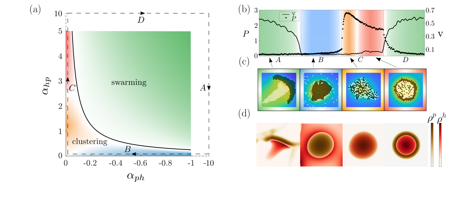
To see in which parameter regimes each of these patterns prevails, in Fig. 3 we show a slice through the state diagram in the plane of the chemotactic cross-species coupling coefficients and . Here we fix and so that prey-particles chemo-attract each other whereas the hunter-particles do not, but note that the specific values choosen here do not have much impact on the emerging patterns.
Hunting Swarms: The green area in Figs. 3(a,b,c) (movies 1,5) represents the hunting-swarm phase which generically occurs if is large enough, as we will later show using a linear stability analysis. Here the chemicals produced by the black-coloured particles in Fig. 2(a) (“prey”) attract the white coloured particles (“hunters”), whereas the hunter-produced chemicals repel the prey. This results in a swarm of “prey” pursued by a swarm of “hunters”. When two or more prey-swarms collide, the pursuing hunters produce a “cage” of high chemical density repelling the prey and trapping it temporarily in a small spatial domain. The prey then ’evades’ sidewards to escape from the hunter-fronts, forming new swarms moving perpendicular to the original ones (see movies 1,5).
Core-shell clusters: When decreasing (blue domain in Figs. 3(a,b) and movies 2,6), so that the prey chemo-attracts the hunters only weakly, we observe that the prey aggregates and forms dense clusters, surrounded by a diffusive corona of hunters. Surprisingly, when staying with a large but decreasing instead (red domain in Figs. 3(a,b,c)), so that the hunters are strongly chemo-attracted by the prey, but the prey has only a weak tendency to avoid the hunter-produced chemicals, we see the opposite case: Although not attracting each other, the hunter-particles form a dense core, surrounded by the prey-particles (red domain in Fig. 3(c) and right panel of Fig. 3(d) and movies 4,8). To see how these remarkable clusters emerge, let us explore the dynamics underlying their formation. Initially, the prey-particles, which chemo-attract each other aggregate and form very small clusters. This leads to an enhanced chemical production, also attracting the hunters, which subsequently invade the cluster, because . Consequently, as more and more hunters enter the cluster, the density of increases in the cluster center, repelling the prey. Since the prey-particles, in turn, couple stronger to their self-produced chemicals than to those produced by the hunters , they do not flee from the cluster but try to stay together. While in the simulations underlying Fig. 2, the hunters invade even small prey-clusters, for appropriate initial conditions, we can see a proper inside out reversal of comparatively large clusters (movie 9) (species reversal). In each case, the result is a counterintuitive pattern consisting of a dense cluster containing mostly hunters surrounded by ring of prey-particles.
Irregular aggregation: Finally, when , are both small, with (orange regime in Figs. 3(a,b) and movies 3,7), prey and hunter particles form clusters containing a seemingly irregular mixture of hunter and prey particles (Fig. 3(c), orange). These clusters emerge because we have a chemically mediated prey-prey attraction and a hunter-by-prey attraction which exceeds the prey-by-hunter-repulsion, so that effectively prey particles similarly strongly attract all other particles, leading to a rather irregular aggregation.
Classification: In contrast to the static clusters, structures in the green region of Fig. 3(a) move ballistically and hence show a non-vanishing velocity. Figure 3(b) depicts the mean particle velocity (see SI for details) at late times for parameters chosen along the dashed line in Fig. 3(a), where one can easily see how the velocity in regions of hunting swarms exceeds that in other regimes. While the hunting swarm phase, which emerges from an oscillatory instability, as discussed further below, can be clearly distinguished from the stationary cluster phases, let us define an “order parameter” to distinguish the remaining cluster phases. We define as the average number of black next neighbors (prey) per white particle (hunter), where we denote a neighbor as a particle within a distance . Figure 3(b) shows for parameters chosen along the dashed line in Fig. 3(a). This parameter would have a value of for completely irregular and infinitely large dense clusters. For the orange domain, where particles aggregate almost irregularly, it has a value , whereas red means () and blue means . Crossover regions between the individual patterns are marked by white domains in Fig. 3(a).
III Linear stability analysis – emergence and dynamics of patterns at early times
To understand the structure of the state diagram we now introduce a continuum description for the particle dynamics and perform a linear stability analysis.
Continuum model: The Smoluchowski equation, describing the dynamics of the (non-normalized) probability to find a particle of species at position at time reads as follows ():
| (5) |
These deterministic equations are equivalent to the Langevin equations (1) for point particles (). We can now also rewrite the evolution equation for the chemical fields as follows:
| (6) |
Before carrying out a linear stability analysis, let us solve these equations numerically to test them: Integrating Eqs. (5, 6) for a uniform initial state (plus small fluctuations) on a square box of size , we indeed find the same patterns as in our particle based simulations (Figs. 2(e-h) and Fig. 3) (see SI for details regarding these simulations and the used method to stabilize them).
Linear stability analysis: We now linearize these four coupled equations around the stationary solution , which represents the uniform disordered phase, and solve them in Fourier Space, to understand the dynamics of a small plane wave perturbation with wavenumber around the uniform phase. We denote the dispersion relation of these fluctuations as . If has a positive real part for some value, the uniform phase is unstable. Calculating (see Supplementary Material for details), we find that the uniform phase looses stability if
| (7) |
where we have choosen as in our simulations. This criterion is consistent with all simulations shown in Fig. 3 and quantitatively agrees with additional simulations which we have performed (not shown). The instability criterion shows that chemo-attractions among the prey particles support the emergence of a pattern in competition with diffusion and the potential decay of the chemical, whereas cross interactions only support the emergence of a pattern if they, and , have the same sign.
To understand the transition between static clusters and hunting swarms, we also derive a criterion discriminating between stationary instability (static clusters, is real) and oscillatory instabilities (moving structures, complex ) which reads as follows (see SI):
| (8) |
This criterion defines the solid black line in Fig. 3(a), which quantitatively agrees with our simulations. It shows that an oscillatory instability and hence moving patterns can appear only if , have opposite sign, i.e. if one species effectively hunts the other one, whereas the other one tries to escape.
In Fig. 4 we show the complete dispersion relation (real and imaginary part) of small plane wave fluctuations around the uniform phase. Here the location of the maxima in define the fastest growing mode, typically determining the length scale of the pattern at early times.
Having understood the transition line between the cluster phases and the hunting swarms, let us also explore if we can understand how fast the swarms move. To do this, in Fig. 5, we compare the imaginary part of (the expected speed of the hunting swarm is ) with the velocity of the hunting swarms in our particle based simulations at early times and find close agreement.
IV Structure and growth at late times
Having explored how the patterns emerge and behave at early times, we now want to explore their structure and dynamics also at late times. To do this, we introduce the instantaneous pair-correlation function defined as
| (9) |
for an average number density with box length , total number of particles and denoting the ensemble average. The radially averaged and time averaged pair-correlation function , where , shown in Fig. 6 describes how the density varies as a function of distance from a reference particle at which we averaged over all particles of hunters and prey.
As one can see in the inset of Fig. 6, there is a large peak around , which is the typical distance between two particles ( in dimensionless units). We can also find peaks around and caused by the next two neighbors. This reflects the fact that the static clusters (blue, orange, red) show a hexagonal packing.
Late-stage dynamics: Once the patterns have emerged, they reach a state where their morphology changes only slowly. However, even at late stages the size of the individual structures still increases in time, partly due to diffusive processes (coarsening), partly due to “collisions“ of different clusters (coalescence).
To quantify this growth, we consider the time evolution of the radial distribution function and define the length scale of clusters as the smallest value where , for all . Thus, the shown in Fig. 6 corresponds to a length scale of (dimensionless units). At late-times, we find that follows a power law with an exponent of (Fig. 7) for the (nonmoving) cluster phases, which is close to the value of as expected for diffusive growth (in the absence of hydrodynamic interactions) Lifshitz and Slyozov 1961; Bray 2002; Gonnella et al. 2015; Laradji and Sunil Kumar 2005; Camley and Brown 2011. We find a much larger exponent, of (Fig. 7), for the patterns in the green region, which is a consequence of the fact that the individual structures move ballistically, collide and merge with each other much faster (but also break up).
As a second measure for the growth of the clusters, we measure the distance between them. To do this, we consider the structure factor of the system:
| (10) |
and calculate the distance between clusters as the inverse of the first moment of the structure factor Stenhammar et al. 2013, i.e. as:
| (11) |
where we choose the cutoff wavelength as the first local minimum of Stenhammar et al. 2013. Figure 8 shows the structure factor for a cluster in the red region of Fig. 3(a) at time for small values of . The peaks that can be seen in the inset of Fig. 8 correspond to the distance of two possible lattice planes of the hexagonal structure. The peak at results from the minimum distance between two particles (). One finds a huge peak around with which we can estimate a typical length, ; the enormous size of the peak hinges on the fact that each of the contributing clusters contains a large number of particles. The -value where this peak occurs corresponds to the mean cluster distance, which corresponds to the value of where approaches from below (see Fig. 6). This distance grows basically with the same power law as the cluster sizes, as shown in Fig. 7, i.e. calculating cluster sizes via and calculating cluster-distances basically leads to the same growth law (Fig. 7) Stanich et al. 2013. Thus, there is only one independent macroscopic length scale in the system.
V Conclusions
Inspired by the generic presence of multi-species chemotaxis in microbiological communities, e.g. in macrophage-tumor cell systems, we have proposed and explored a physical minimal model to study the collective behaviour beyond the commonly considered one-species limit. We have found that the novel key ingredient of our model - the species selective chemical production - leads to patterns which have so-far been known only to occur within the animal kingdom at much larger scales, e.g. in insects and larvae-crustacean-systems: these patterns comprise a “hunting swarm” phase consisting of a crowd of particles of one species pursuing the other species, and a phase where the two-species self-aggregate in a core-shell structure, which may feature a dynamical inside-out reversal en route to the steady state.
All these patterns could be observed both on the level of a particle-based description (Eqs. (3, 4) and in a continuum model (Eqs. (5, 6)), allowing to analytically understand the transition line between cluster phases, which originate from a stationary instability of the uniform phase, and hunting swarms, emerging from an oscillatory instability. As a further characteristic difference between these phases, we find that clusters (and the distance between them) grow diffusively ( Stanich et al. 2013; Lifshitz and Slyozov 1961; Bray 2002; Gonnella et al. 2015; Laradji and Sunil Kumar 2005; Camley and Brown 2011), whereas hunting swarms grow significantly faster ( Cremer and Löwen 2014).
Future work might include more specific biological details and could address the effect of confining boundaries or obstacles Morin et al. 2016; Toner et al. 2018; Huang et al. 2017b; Rahmani et al. 2019. Other topics concern additional aligning interactions and their impact on the cluster structure Das 2017; Mones et al. 2015; Nilsson and Volpe 2017 and ternary systems describing species of a longer biological food chain.
Data availability
All relevant data are available from the authors upon reasonable request.
References
- Čejková et al. (2017) J. Čejková, S. Holler, T. Q. Nguyenová, C. Kerrigan, F. Štěpánek, and M. M. Hanczyc, in Advances in Unconventional Computing (Springer, 2017).
- H Wadhams and P Armitage (2005) G. H Wadhams and J. P Armitage, Making sense of it all: bacterial chemotaxis, Nat. Rev. Mol. Cell Biol. 5, 1024 (2005).
- Eidi et al. (2017) Z. Eidi, F. Mohammad-Rafiee, M. Khorrami, and A. Gholami, Modelling of Dictyostelium discoideum movement in a linear gradient of chemoattractant, Soft Matter 13, 8209 (2017).
- Laganenka et al. (2016) L. Laganenka, R. Colin, and V. Sourjik, Chemotaxis towards autoinducer 2 mediates autoaggregation in Escherichia coli, Nat. Commun. 7, 12984 EP (2016), article.
- Tindall et al. (2008) M. J. Tindall, P. K. Maini, S. L. Porter, and J. P. Armitage, Overview of mathematical approaches used to model bacterial chemotaxis II: bacterial populations, Bull. Math. Biol. 70, 1570 (2008).
- Murray (2003) J. D. Murray, Bacterial Patterns and Chemotaxis, in Mathematical Biology: II: Spatial Models and Biomedical Applications, edited by J. D. Murray (Springer New York, New York, NY, 2003).
- Hillen and Painter (2008) T. Hillen and K. J. Painter, A user’s guide to PDE models for chemotaxis, J. Math. Biol. 58, 183 (2008).
- Painter (2018) K. J. Painter, Mathematical models for chemotaxis and their applications in self-organisation phenomena, J. Theor. Biol. (2018).
- Painter and Hillen (2011) K. J. Painter and T. Hillen, Spatio-temporal chaos in a chemotaxis model, Phys. D 240, 363 (2011).
- Dolak and Schmeiser (2005) Y. Dolak and C. Schmeiser, Kinetic models for chemotaxis: Hydrodynamic limits and spatio-temporal mechanisms, J. Math. Biol. 51, 595 (2005).
- Mukherjee and Ghosh (2018) M. Mukherjee and P. Ghosh, Growth-mediated autochemotactic pattern formation in self-propelling bacteria, Phys. Rev. E 97, 012413 (2018).
- Bergmann et al. (2018) F. Bergmann, L. Rapp, and W. Zimmermann, Active phase separation: A universal approach, Phys. Rev. E 98, 020603 (2018).
- Knútsdóttir et al. (2014) H. Knútsdóttir, E. Palsson, and L. Edelstein-Keshet, Mathematical model of macrophage-facilitated breast cancer cells invasion, J. Theor. Biol. 357, 184–199 (2014).
- Stark (2018) H. Stark, Artificial Chemotaxis of Self-Phoretic Active Colloids: Collective Behavior, Acc. Chem. Res. 51, 2681 (2018).
- Robertson et al. (2018) B. Robertson, M.-J. Huang, J.-X. Chen, and R. Kapral, Synthetic Nanomotors: Working Together through Chemistry, Acc. Chem. Res. 51, 2355 (2018).
- Liebchen and Löwen (2018) B. Liebchen and H. Löwen, Synthetic Chemotaxis and Collective Behavior in Active Matter, Acc. Chem. Res. 51, 2982 (2018).
- Marchetti et al. (2013) M. C. Marchetti, J. F. Joanny, S. Ramaswamy, T. B. Liverpool, J. Prost, M. Rao, and R. A. Simha, Hydrodynamics of soft active matter, Rev. Mod. Phys. 85, 1143 (2013).
- Romanczuk et al. (2012) P. Romanczuk, M. Bär, W. Ebeling, B. Lindner, and L. Schimansky-Geier, Active Brownian particles, Eur. Phys. J.-Spec. Top. 202, 1 (2012).
- Kurzthaler et al. (2018) C. Kurzthaler, C. Devailly, J. Arlt, T. Franosch, W. C. K. Poon, V. A. Martinez, and A. T. Brown, Probing the Spatiotemporal Dynamics of Catalytic Janus Particles with Single-Particle Tracking and Differential Dynamic Microscopy, Phys. Rev. Lett. 121, 078001 (2018).
- Bechinger et al. (2016) C. Bechinger, R. Di Leonardo, H. Löwen, C. Reichhardt, G. Volpe, and G. Volpe, Active particles in complex and crowded environments, Rev. Mod. Phys. 88, 045006 (2016).
- Aranson (2013) I. S. Aranson, Active colloids, Phys.-Usp. 56, 79 (2013).
- Saha et al. (2014) S. Saha, R. Golestanian, and S. Ramaswamy, Clusters, asters, and collective oscillations in chemotactic colloids, Phys. Rev. E 89, 062316 (2014).
- Pohl and Stark (2014) O. Pohl and H. Stark, Dynamic Clustering and Chemotactic Collapse of Self-Phoretic Active Particles, Phys. Rev. Lett. 112, 238303 (2014).
- Liebchen et al. (2015) B. Liebchen, D. Marenduzzo, I. Pagonabarraga, and M. Cates, Clustering and Pattern Formation in Chemorepulsive Active Colloids, Phys. Rev. Lett. 115, 258301 (2015).
- Liebchen et al. (2017) B. Liebchen, D. Marenduzzo, and M. Cates, Phoretic Interactions Generically Induce Dynamic Clusters and Wave Patterns in Active Colloids, Phys. Rev. Lett. 118, 268001 (2017).
- Huang et al. (2017a) M.-J. Huang, J. Schofield, and R. Kapral, Chemotactic and hydrodynamic effects on collective dynamics of self-diffusiophoretic Janus motors, New J. Phys. 19, 125003 (2017a).
- Liebchen and Löwen (2019) B. Liebchen and H. Löwen, Which interactions dominate in active colloids? J. Chem. Phys. 150, 061102 (2019).
- Soto and Golestanian (2014) R. Soto and R. Golestanian, Self-Assembly of Catalytically Active Colloidal Molecules: Tailoring Activity Through Surface Chemistry, Phys. Rev. Lett. 112, 068301 (2014).
- Schmidt et al. (2019) F. Schmidt, B. Liebchen, H. Löwen, and G. Volpe, Light-controlled assembly of active colloidal molecules, J. Chem. Phys. 150, 094905 (2019).
- Niu et al. (2017) R. Niu, T. Palberg, and T. Speck, Self-Assembly of Colloidal Molecules due to Self-Generated Flow, Phys. Rev. Lett. 119, 028001 (2017).
- Stürmer et al. (2019) J. Stürmer, M. Seyrich, and H. Stark, Chemotaxis in a binary mixture of active and passive particles, J. Chem. Phys. 150, 214901 (2019).
- Singh et al. (2017) D. P. Singh, U. Choudhury, P. Fischer, and A. G. Mark, Non-Equilibrium Assembly of Light-Activated Colloidal Mixtures, Advanced Materials 29, 1701328 (2017).
- Agudo-Canalejo and Golestanian (2019) J. Agudo-Canalejo and R. Golestanian, Active Phase Separation in Mixtures of Chemically Interacting Particles, Phys. Rev. Lett. 123, 018101 (2019).
- Wang et al. (2018) L. Wang, M. N. Popescu, F. Stavale, A. Ali, T. Gemming, and J. Simmchen, Cu@TiO2 Janus microswimmers with a versatile motion mechanism, Soft Matter 14, 6969 (2018).
- Ivlev et al. (2015) A. Ivlev, J. Bartnick, M. Heinen, C.-R. Du, V. Nosenko, and H. Löwen, Statistical mechanics where Newton’s third law is broken, Phys. Rev. X 5, 011035 (2015).
- Sengupta et al. (2011) A. Sengupta, T. Kruppa, and H. Löwen, Chemotactic predator-prey dynamics, Phys. Rev. E 83, 031914 (2011).
- Boonman et al. (2019) A. Boonman, Y. Yovel, and B. Fenton, The benefits of insect-swarm hunting in echolocating bats, and its influence on the evolution of bat echolocation signals, bioRxiv , 554055 (2019).
- Jeschke and Tollrian (2007) J. M. Jeschke and R. Tollrian, Prey swarming: which predators become confused and why? Animal Behaviour 74, 387 (2007).
- Zhdankin and Sprott (2010) V. Zhdankin and J. C. Sprott, Simple predator-prey swarming model, Phys. Rev. E 82, 056209 (2010).
- Höhn et al. (2015) S. Höhn, A. R. Honerkamp-Smith, P. A. Haas, P. K. Trong, and R. E. Goldstein, Dynamics of a Volvox Embryo Turning Itself Inside Out, Phys. Rev. Lett. 114, 178101 (2015).
- Lifshitz and Slyozov (1961) I. Lifshitz and V. Slyozov, The kinetics of precipitation from supersaturated solid solutions, J. Phys. Chem. Solids 19, 35 (1961).
- Bray (2002) A. J. Bray, Theory of phase-ordering kinetics, Adv. Phys. 51, 481 (2002).
- Gonnella et al. (2015) G. Gonnella, D. Marenduzzo, A. Suma, and A. Tiribocchi, Motility-induced phase separation and coarsening in active matter, C. R. Phys. 16, 316 (2015).
- Laradji and Sunil Kumar (2005) M. Laradji and P. B. Sunil Kumar, Domain growth, budding, and fission in phase-separating self-assembled fluid bilayers, J. Chem. Phys. 123, 224902 (2005).
- Camley and Brown (2011) B. A. Camley and F. L. H. Brown, Dynamic scaling in phase separation kinetics for quasi-two-dimensional membranes, J. Chem. Phys. 135, 225106 (2011).
- Stenhammar et al. (2013) J. Stenhammar, A. Tiribocchi, R. J. Allen, D. Marenduzzo, and M. E. Cates, Continuum Theory of Phase Separation Kinetics for Active Brownian Particles, Phys. Rev. Lett. 111, 145702 (2013).
- Stanich et al. (2013) C. Stanich, A. Honerkamp-Smith, G. Putzel, C. Warth, A. Lamprecht, P. Mandal, E. Mann, T.-A. Hua, and S. Keller, Coarsening Dynamics of Domains in Lipid Membranes, Biophys. J. 105, 444 (2013).
- Cremer and Löwen (2014) P. Cremer and H. Löwen, Scaling of cluster growth for coagulating active particles, Phys. Rev. E 89, 022307 (2014).
- Morin et al. (2016) A. Morin, N. Desreumaux, J.-B. Caussin, and D. Bartolo, Distortion and destruction of colloidal flocks in disordered environments, Nat. Phys. 13, 63 EP (2016).
- Toner et al. (2018) J. Toner, N. Guttenberg, and Y. Tu, Hydrodynamic theory of flocking in the presence of quenched disorder, Phys. Rev. E 98, 062604 (2018).
- Huang et al. (2017b) M.-J. Huang, J. Schofield, and R. Kapral, Transport in active systems crowded by obstacles, J. Phys. A: Math. Theor. 50, 074001 (2017b).
- Rahmani et al. (2019) P. Rahmani, F. Peruani, and P. Romanczuk, Flocking in complex environments – attention trade-offs in collective information processing, arXiv:1907.11691 [physics.bio-ph] (2019).
- Das (2017) S. K. Das, Pattern, growth, and aging in aggregation kinetics of a Vicsek-like active matter model, J. Chem. Phys. 146, 044902 (2017).
- Mones et al. (2015) E. Mones, A. Czirók, and T. Vicsek, Anomalous segregation dynamics of self-propelled particles, New J. Phys. 17, 063013 (2015).
- Nilsson and Volpe (2017) S. Nilsson and G. Volpe, Metastable clusters and channels formed by active particles with aligning interactions, New J. Phys. 19, 115008 (2017).
Author contributions
H.L. and B.L. have planned and designed the research project; J.G. has performed most of the research; all authors have discussed the results; J.G. and B.L. have written the manuscript; H.L. and A.B. have edited it.