The vulnerability of communities in complex network: An entropy approachJournal: Reliability Engineering & System Safety
Abstract
Measuring the vulnerability of communities in complex network has become an important topic in the research of complex system. Numerous existing vulnerability measures have been proposed to solve such problems, however, most of these methods have their own shortcomings and limitations. Therefore, a new entropy-based approach is proposed in this paper to address such problems. This measure combines the internal factors and external factors for each communities which can give the quantitative description of vulnerability of community. The internal factors contain the complexity degree of community and the number of edges inside the community, and the external factors contain the similarity degree between chosen community and other communities and the number of nodes outside the community. Considering community vulnerability from the perspective of entropy provides a new solution to such problem. Due to sufficient consideration of community information, more reasonable vulnerability result can be obtained. In order to show the performance and effectiveness of this proposed method, one example network and three real-world complex network is used to compare with some exiting methods, and the sensitivity of weight factors is analysed by Sobol’ indices. The experiment results demonstrate the reasonableness and superiority of this proposed method.
Keywords:
Complex network, Community vulnerability, Entropy1 Introduction
Recently, cyber-physical system (CPS) has attracted much attention in numerous fields, such as microgrid Guan2010Microgrid, smart city BRUNEO201912service, internet of things Dautov2019Hierarchical, Dautov2018Metropolitan, and so on. Meanwhile, how to model CPS into specific physical models to analyze their performance and property has become the focus of research Lee2019cascading. Therefore, complex network has been applied in this field to better understand the performance of CPS Cheng2019Smart, Guo2019network, because nodes in the network represent individuals in the system, and edges would show the relationship between these individuals. Most of previous researches focus on the structure and topological property, which can quantify the characteristic and performance of network. Particularly, the community structure has received increasing attention, because it can reveal human dynamics wang2018exploiting, wang2017onymity, inference reliable links Ma2019Reliable, and identify influential nodes ZHANG2019249, wentao2019nodes. The community structure in the network demonstrates a higher density of nodes and edges, which can cause critical influence on the function and structure of subnetwork, improve the reliability of system DUI2019162System, LEVITIN2019289Optimization, and counteract the aging effect LEVITIN2019397Dynamic, LEVITIN201963Joint.
There are several different problems about the research of community structure, which can be divided into two issues. The first one is about the structure of community, such as dividing network’s community structure Zhu2019Community, Orman2015Interpreting, Rocco2017Effects, detecting overlapping community Orman2015Overlapping, and dynamic changes of community in evolving network ORMAN2017375. Another one is the property of community, including measuring the reliance of community Ramirez2018Quantifying, Zhang2018uncertainty, Cerqueti2019resilience, reconfiguring network Zhang2019Reconfiguration, quantifying the reliability of communityRamirez2016Robustness, Zhang2017Reliability, and measuring community vulnerability wentao2018evaluating. The vulnerability of community in network gradually aroused researchers’ interest recently. For example, Rocco et al. Rocco2011Vulnerability defined vulnerability set and value for different community, and proposed relative vulnerability value to compare with remaining communities. Wei et al. Wei2018Measuring proposed a measure which consider more information about community itself, and used non-linear weighted function to combine these factors. Aniko et al. Kovacs2019vulnerability proposed a topological index (distance-based fragmentation) to quantify the structural vulnerability in plant-visitation network. Alim et al. Alim2016Structural assessed the community vulnerability through social-based forwarding and routing methods in opportunistic networks, which shows significant contribution about some devices on the performance of entire network. Che et al. Yanbo2019Vulnerability modified original evolution method, and proposed a nondimensionalized scoring standard to form a complete assessment system to measure the vulnerability of urban power grid. Chen et al. CHEN2019CORRELATION explored the relationship between vulnerability of complex network and fractal dimension. These methods have their own limitations, like computational complexity, inaccurate measurements, and not suitable for certain scenarios.
Since entropy is an useful tool to measure the uncertain of information Dengwei2018, wang2016statistical, it has been wildly in the network theory, like dimension presentation wb2019, WU2018HADAMARD, wentao2018information, evidence theory jiang2018Correlation, Jiang2019Znetwork, influential nodes identification li2018evidential, wang2018amodified, time series prediction xu2018visibility, Fan2019timeseries. In addition, the structure and property of communities can be expressed by probability sets, entropy-based method has gradually been an reasonable and effective method to quantify the property of network wentao2019similar, wentao2019structure. Therefore, an entropy approach is applied in this paper to measure the vulnerability of community which can overcome the shortcomings and limitations of previous method.
In this paper, an entropy-based measure is proposed to quantify the vulnerability degree of community structure. This proposed method can combine two parts of information, i.e., internal factors and external factors, which can consider more information about community and give a reasonable vulnerability result of each community. The internal factors contains the number of edges inside the community and the complexity degree of community which is measured by Tsallis structure entropy, and the external factors contains the number of edges outside the community and the similarity degree between chosen community and other communities which is measured by relative entropy. These two entropy can quantify the property of community more reasonable and effective. Finally, the vulnerability and relative vulnerability result can be obtained by this proposed method to quantitatively describe vulnerability of different community. In order to show the performance and effectiveness of this proposed method, one example network and three real-world complex network are applied in this paper. In addition, the sensitive of four weight factors are analysed by Sobol’ indices in Manzi network, and the vulnerability order obtained by different method are compared in Italian 380KV power grid network. The experiments results show the superiority and reasonableness of this proposed method, meanwhile, this proposed method can overcome the shortcomings and limitations of previous method,
The organization of the rest of this paper is as follows. Section 2 presents some basic properties about node and detecting community methods. This novel entropy-based method is proposed in Section 3 to measure the vulnerability of community. Meanwhile, numerical experiments are performed to illustrate the reasonableness and effectiveness of the proposed method in Section 4. Conclusion is conducted in Section 5.
2 Preliminaries
In this section, some basic concepts about complex network are introduced. In addition, a community detection algorithm and classical community vulnerability measure are described in this section.
2.1 Node properties in network
A given complex network can be denoted as , where and is the set of nodes and edges respectively, and and is the number of nodes and edges in the complex network respectively. is the adjacency matrix of complex network whose size is , where represents there is an edge between node and node , and is the opposite.
Definition 2.1.
(Node Degree). The degree of node in the complex network is denoted as and defined as follows,
| (1) |
where is one element of adjacency matrix . The degree distribution of node is defined as follows,
| (2) |
Definition 2.2.
(Node Betweenness). The betweenness distribution of node in the complex network is denoted as and defined as follows,
| (3) |
where is the total number of shortest paths between node and node , and is the number of shortest paths between node and node which pass through node .
2.2 Community detection algorithm
Lots of measures have been proposed to detect the community structure in complex network. In order to find the community structure of network, Newman’s modularity method Newman2004Fast is applied in this paper.
Definition 2.3.
(Newman’s modularity). For a given complex network with communities, the modularity is denoted as and defined as follows,
| (4) |
where is the number of communities, is the total number of edges in complex network, is the number of edges in community , and is the total degree of nodes in community which is defined as follows,
| (5) |
where is the set of nodes in community, and is the degree of node .
The value of can measure the difference of different communities which can show the presence of community structure in complex network. Different value of represents different situation. means all of the nodes in the network are in one single community and there is no community structure in the network. represents there are some kinds of community structure, and means the community structure is strong in the network. Meanwhile, Newman and Girvan Newman2004Finding suggested the value of should fall in the range , and this value of would show the existence of community structures.
The main idea of this method is to find the changes in , and the step to detect community structure is shown as follows,
Step 1: Each node in the complex network is divided in a single community.
Step 2: Every two communities are integrated into one community in turn, and the value of modularity change can obtained from the community structure.
Step 3: Community and community are integrated into one community with the highest .
Step 4: Repeat Step 2 and Step 3 until .
2.3 Classical community vulnerability measure
To measure the vulnerability of community, lots of measures have been proposed. One classical measure is introduced in this section.
Definition 2.4.
(Community vulnerability measure). The vulnerability of community is denoted as and defined as follows,
| (6) |
where is the set of communities which are connected with community , and is the number of links which are connected with community .
The relative vulnerability of community is denoted as and defined as follows,
| (7) |
3 The proposed method
3.1 Basic method
In this section, a novel method is proposed to measure community vulnerability via entropy approach. This proposed method focuses two parts of information which can consider more details in the network, including internal factors and external factors. The internal factors include the complexity degree of community and number of edges within the community, and external factors include the similarity degree and number of edges between chosen community and other communities. The complexity and similarity would be obtained by entropy method which would overcome the shortcomings and limitations of previous method. The flow chart of this proposed method is shown in Fig. 1.

3.1.1 Complexity measure
Firstly, the complexity degree of community is measured by Tsallis structure entropy which combines the degree distribution and betweenness distribution. Because degree distribution focuses on the local topological information of central node and betweenness distribution considers the global topological information, Tsallis structure entropy which combines these two topological information can give a reasonable measure for community complexity.
Definition 3.1.
(Complexity measure based on Tsallis structure entropy). The complexity degree of community is denoted as and defined as follows,
| (8) |
where is the number of nodes in community , is the degree distribution node which can be obtained by Eq. (2), can be obtained from betweenness distribution, and the relationship between and is shown as follows,
| (9) |
where can be obtained from Eq. (3), is the maximum value of betweenness . The purpose of Eq. (9) is to make the index bigger than 1 which can show the influence of subnetwork to community .
When each node’s equals to 1, Tsallis entropy would degenerate to Shannon entropy which is shown as follows,
| (10) |
This form of entropy would only focuses on the local topological structure information.
The degree distribution is based on the local topological structure around central node . The betweenness distribution focuses on the whole topological structure which can describe the global properties of community. Most of time, would be bigger than 1 which can show the influence of subnetwork. When each nodes’s equals to 1, the Tsallis entropy would degenerate to Shannon entropy based on degree distribution which only focuses on the local structure. Using betweenness distribution to replace the constant parameter can describe the information about the network itself which is more reasonable for measuring the communities’ complexity. This method’s property also obeys the classical Tsallis entropy.
3.1.2 Similarity measure
Then, relative entropy is used in this section to obtain the similarity degree of chosen community and other communities. The relative entropy (KullbackLeibler divergence) was wildly used in information theory and probability theory which is proposed by Kullback and Leibler et al. Kullback1951ON. In general, the relative entropy is used to measure the difference between two probability set. In this section, the relative entropy is based on Shannon entropy and degree distribution which can measure the similarity between two community structure.
For two community and , the community structure is denoted as and respectively, where and is the set of nodes and set of degree of nodes in community . is the number of nodes in community and is the maximum size of community in the network. The probability set of community is denoted as and obtained by degree distribution. The scale of every probability set would be same which equals to . So the probability set of community can be shown as follows,
| (11) |
The element in probability set is based on degree distribution. When the size of community equals to , all of the elements would be obtained by nodes’ degree, but when , some elements would equal to zero to make the probability set complete. The detail of is defined as follows,
| (12) |
where is the degree of node , is the number of nods in community .
To measure the similarity between community and , the relative entropy is used in this section and it is defined as follows,
Definition 3.2.
(Similarity measure based on relative entropy). The difference between two communities is obtained by relative entropy and defined as follows,
| (13) |
Because the order of element would affect the relative entropy and similarity result, and are the decreasing order of and in Eq. (11). can be obtained as follows,
| (14) |
The adjustment of is to avoid being 0 or positive infinity, which would be beneficial for calculation. The relative entropy’ property is not symmetry, so the following changes are needed to make it symmetrical,
| (15) |
Thus, holds, and the relative entropy between two communities are symmetry. Because the relative entropy measure the difference between two probability set, the difference between two communities are obtained in this situation. The bigger , the greater the difference between two communities structure is. So the similarity index is obtained based on relative entropy to show the similarity between two communities, and it is denoted as and defined as follows,
| (16) |
where is also symmetry, and shows the similarity between two communities structure. The more similar the two communities, the less the difference between them is, the closer is to and the closer is to zero.
So the similarity between two communities structure can be measured by the relative entropy, which can give a novel approach to this problem. The relative entropy focuses on the local structure topological information in the community structure, which is more reasonable.
3.1.3 Edges in the network
The number of edges inside and outside the community are also important for community vulnerability measuring. In this section, the number of edges is considered.
Definition 3.3.
(Number of edges inside the community). The number of edges inside the community is donated as and defined as follows,
| (17) |
where node and node are within the community , is the element of adjacency matrix . Thus, is entirely inside the community.
Definition 3.4.
(Number of edges outside the community). The number of edges outside the community is donated as and defined as follows,
| (18) |
where node is within the community , and node is outside the community , is the element of adjacency matrix . Thus, connects the chosen community and other communities which can show the relationship between them.
3.1.4 Community vulnerability measure
Lastly, all of the factors defined in Definition 3.1 to 3.4 are considered in the vulnerability measuring model. This proposed method would consider the internal factors and external factors which consider more details of community, and is defined as follows,
Definition 3.5.
(Proposed community vulnerability measure). The vulnerability of community is donated as and defined as follows,
| (19) |
where are the weight factors of different parameters, and all of them are bigger than zero. and is the number of edges inside and outside the community respectively, is the complexity degree of community , and represents the similarity degree between community and other communities (exclude community itself) which can be shown as follows,
| (20) |
where can be obtained by Eq. (16)
The relative vulnerability of community is denoted as and defined as follows,
| (21) |
In order for these parameters to be considered on the same scale, all of these four parameters are normalized firstly. The weight factors can give the weight to consider different parameters, which can be adjusted in different situation. This setting of weight factor makes this proposed method more reasonable. Some special cases of this proposed method are shown as follows,
1) When , this four parameters are considered equally.
2) When , and , this proposed method would degenerate to the classical vulnerability measure in Eq. (6).
3) When , this proposed method would consider the external factors, which is the communities connected with chosen community.
4) When , this proposed method would only consider the internal factors, i.e., the chosen community.
3.2 Sensitive analysis
Because these four weight factors () are important for community vulnerability measuring, and the vulnerability result would have a related changes as weight factors change, thus, how to determine factors has been a problem in this model. In this section, the sensitive of these weight factors are analysed. In general, the global sensitivity analysis ia a useful tool to obtain the influence of inputs on the output variability in mathematical and physical model, and Sobol’ indices based on variance decomposition is applied in this paper. The first-order Sobol’ index and total effect index are defined as follows respectively,
| (22) |
| (23) |
where represents the output of system, is the th independent input , is all of the inputs exclude , is the variance which change with these inputs. The first-order Sobol’ index can get the contribution of to , and total effect index can get the contribution to the variance of by the variability of each input , which considering its individual effects and the interaction with other variables.
Each weight factors are randomly generated 10000 times by Monte Carlo method, and the range fall into [0.2, 5]. The vulnerability result would be obtained by these random factor combinations, and the contribution of different weight factors can be obtained by first-order Sobol’ index and total effect index.
3.3 An illustrative example
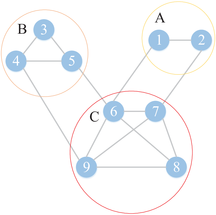
In this section, an example network is given to show the difference between this proposed method and classical measure . The network structure is shown in Fig. 2. Observing from Fig. 2, this network has 9 nodes and 14 edges, and the community structure of network is detected by Newman’s modularity in Eq. (4). The network is divided into three communities () and each of the community is a fully-connected subnetwork. All of these four weight factors equal to one which make four parameters equally important. According to this proposed method in Eq. (19), (21) and classical measure in Eq. (6), (7), four parameters and the vulnerability of three communities are shown in Table 1.
| Community | |||||||||
|---|---|---|---|---|---|---|---|---|---|
| Community A | 1 | 0.5 | 0.1667 | 0.5 | 0.5 | 24 | 27.6264 | 2 | 2 |
| Community B | 0.4298 | 0.7924 | 0.5 | 0.5 | 0.5 | 2.1696 | 2.4975 | 2 | 2 |
| Community C | 0.8687 | 1 | 1 | 1 | 1 | 0.8687 | 1 | 1 | 1 |
From Table 1 when , it can be found that the vulnerability of community C is the lowest, which is the same as the classical measure, but the vulnerability of community A and B is different with classical measure. It can be found from Table 1 that the classical measure of the vulnerability of community A and B is same and it is 2 because of the same number of edges outside of chosen community. However, this classical method is not reasonable, because the vulnerability of one chosen community is determined not only by external factors but also by internal factors. From Fig. 2, community A is a fully-connected subnetwork with only two nodes, but community B is a fully-connected subnetwork with three nodes. When the network’ structure is similar, i.e., fully-connected, the network with more nodes would be more robust, so community B is more robust than community A. The similar vulnerability result can be obtained by this proposed method (), which is more reasonable for real-world application. The relative vulnerability can be more obvious to show the vulnerability difference between different community. From the comparison result of example network, this proposed vulnerability measure outperforms classical method, and can distinguish the vulnerability level of community that the classical method cannot distinguish.
4 Experimental study
In this section, three real-world complex networks are applied to show the performance and effectiveness of this proposed method. These three networks are namely as Manzi network Manzi2001Fishman, Karate network Zachary1977Information, Italian power network Crucitti2005Locating respectively. The topological properties of these three networks are shown in Table 2. Observing from Table 2, and is the number of nodes and edges respectively. and is the average and maximum value of degree respectively, and and is the average and maximum value of shortest distance respectively in the network.
| Network | ||||||
|---|---|---|---|---|---|---|
| Manzi | 52 | 76 | 2.8077 | 5 | 5.5000 | 13 |
| Karate | 34 | 78 | 4.5882 | 17 | 2.4082 | 5 |
| Italian | 127 | 171 | 2.6929 | 7 | 8.5682 | 25 |
4.1 Manzi network
Firstly, the telephone network in Belgium Manzi2001Fishman which was analyzed for reliability purposes is used in this section. The topological structure of this network and the community structure obtained by Newman’s modularity Newman2004Fast is shown in Fig. 3. Observing from Fig. 3, Manzi network is divided into seven communities (), and the detail nodes in each community is shown in Table 3.

The vulnerability of each community can guide the identification of critical community in the network. The vulnerability and relative vulnerability of each community are given in Table 4, the classical comparing vulnerability measure and are also shown in Table 4. Observing classical measure in Table 4, community 7 is the most vulnerable community, but community 3 is the most robust community in the network. The vulnerability of the rest of community (community 1, 2, 4, 5, 6) cannot be identified by the classical measure because of the same value of . Thus, this novel method is proposed based on two parts of information, including internal factors and external factors. The result of this proposed method (, ) are shown in Table 4. It can be found that community 3 is also the most robust community in the network which is same as the classical method. The value of in community 4 and community 7 is close, which are more vulnerable than other communities. The rest of communities can get close but different , which can give a vulnerable order of this community (community 6 community 5 community 2 community 1). The vulnerable order of community in the network is community 4 community 7 community 6 community 5 community 2 community 1 community 3. So this proposed method can consider more information in the network and give a detail vulnerable order for these communities which can overcome some limitations of classical method.
| community | Nodes in community |
|---|---|
| 1 | 3,6,7,8,9,10,13 |
| 2 | 1,2,4,5,11,12,14 |
| 3 | 15,16,17,18,20,21,24,25,29,31 |
| 4 | 19,22,26 |
| 5 | 23,38,30,32,36,37,41,43 |
| 6 | 27,33,34,35,38,39,40,42,45,46,47,49,50 |
| 7 | 44,48,51,52 |
| Community | |||||||||
|---|---|---|---|---|---|---|---|---|---|
| 1 | 0.3518 | 0.6864 | 0.4210 | 0.6667 | 0.6667 | 1.8260 | 1.8775 | 1.5 | 1.5 |
| 2 | 0.3529 | 0.7909 | 0.3684 | 0.6667 | 0.6667 | 1.8170 | 1.8682 | 1.5 | 1.5 |
| 3 | 0.4783 | 0.9344 | 0.5263 | 1 | 1 | 0.9725 | 1 | 1 | 1 |
| 4 | 1 | 0.5447 | 0.1578 | 0.6667 | 0.6667 | 17.4406 | 17.9322 | 1.5 | 1.5 |
| 5 | 0.4139 | 0.8814 | 0.4210 | 0.6667 | 0.6667 | 1.6730 | 1.7202 | 1.5 | 1.5 |
| 6 | 0.7654 | 1 | 1 | 0.6667 | 0.6667 | 1.1482 | 1.1805 | 1.5 | 1.5 |
| 7 | 0.6429 | 0.5915 | 0.2105 | 0.3333 | 0.3333 | 15.4872 | 15.9238 | 3 | 3 |
Then, Sobol’ indices introduced in Section 3.2 is used in this section to analysis the global sensitivity of these four weight factor . These weight factors can adjust the consideration of different parameters which can give a different vulnerability result. The sensitivity analysis result for the vulnerability of different community with different weight factors are shown in Table 5. Some conclusions can be obtained as follows,
1) The value of first-order Sobol’ index can show the sensitivity of different wight factors. For instance, the vulnerability of community 1 is most sensitive to weight factor , followed by , the other two factors and are less sensitive.
2) When the parameters of community equals to one, the first-order Sobol’ index and total effect index would equal to 1. That is because no matter how weight factor change, the influence parameter would remain the same, i.e., equal to 1. For example, and equal to 1 in community 6, so , , and equal to 0. Thus, the variability of these two weight factors would not affect the vulnerability measure of community 6. The same situation can occur in of community 4 and of community 3.
3) In most of communities, the first-order Sobol’ index and are smaller than and , which means the vulnerability measure of community is more sensitive with and . The similarity degree and the number of edges within community are more influential to the vulnerability results.
4) The first-order Sobol’ index , , would be smaller when the value of parameters , , and are bigger, and is different situation which is bigger with bigger parameters . The situation occurs because is positively correlated with , but negatively correlated with , , and . Hence the value trend of these parameters would have different impact on the vulnerability of communities. These patterns can be observed from all of these communities vulnerability sensitivity analysis in Table 5.
5) The sum of the first-order Sobol’ index over these four weight factors in different communities are less than 1, which means there is an interaction between these four parameters. But this situation does not occur in total effect index.
6) Because of the interaction between these parameters, there would be a huge difference between first-order Sobol’ index and total effect index. But it is interesting to find that the order of total effect index would be the same as first-order Sobol’ index. For instance, the order of first-order Sobol’ index in community 1 is , the order of total effect index is , which is same as previous order.
| Community | |||||||||
|---|---|---|---|---|---|---|---|---|---|
| 1 | 0.2055 | 0.7504 | 0.0529 | 0.2604 | 0.1570 | 0.5644 | 0.0294 | 0.2394 | |
| 2 | 0.1983 | 0.7288 | 0.0509 | 0.2655 | 0.1941 | 0.6308 | 0.0114 | 0.1070 | |
| 3 | 0.3969 | 0.6861 | 0 | 0 | 0.3116 | 0.5945 | 0.0044 | 0.0124 | |
| 4 | 0 | 0 | 0.0253 | 0.2524 | 0.4246 | 0.8596 | 0.0883 | 0.4478 | |
| 5 | 0.2229 | 0.6721 | 0.0650 | 0.2812 | 0.2247 | 0.6074 | 0.0048 | 0.0345 | |
| 6 | 0.2895 | 0.3756 | 0.6343 | 0.7163 | 0 | 0 | 0 | 0 | |
| 7 | 0.0275 | 0.3536 | 0.0966 | 0.6666 | 0.1579 | 0.7105 | 0.0374 | 0.3531 |
Because Sobol’ indices is convenient to obtained, and similar results can be obtained from differen network, we only analyse the sensitivity of weight factors in Manzi network and don’t analyse the subsequent network.
4.2 Karate network
Next, a social network is used in this section to show the performance of this proposed method. This social network is named as Karate club network, which describes the relationship between 34 members of one club in US university Zachary1977Information. The topological structure and community structure divided by Newman’s modularity is shown in Fig. 4. Every nodes in the network denote a member in karate club, including the instructors and administrators, and the edges in the network represent the relationship between two members beyond their normal activities in the club. The network is divided into two communities (), and it is same as the well-known community structure result because there has been disagreement between administrators and instructors Zachary1977Information. The detail member in each communities is shown in Table 6, and it can be found that the members are divided equally and each community have 17 members. The leader in each community is node 1 and node 34 respectively because of their largest degree.

| community | Nodes in community |
|---|---|
| 1 | 1, 2, 3, 4, 5, 6, 7, 8, 10, 11, 12, 13, 14, 17, 18, 20, 22 |
| 2 | 9, 15, 16, 19, 21, 23, 24, 25, 26, 27, 28, 29, 30, 31, 32, 33, 34 |
The vulnerability measure result of Karate network is shown in Table 7. Because there is only two communities, it can be found that the external factors (, ) are determined by each other, and they are the same. Thus, the classical measure would obtain same result and cannot identify the vulnerability degree of each community. But the internal factors are determined by community itself, these parameters can get a different result. It is interesting to find that the number of edges inside the community is also same and it is 34, but the edges between nodes are different which result in a different complexity degree. The complexity degree of two communities are 0.7060 and 1 respectively, which would get a different vulnerability measure for different communities. The relative vulnerability of each communities are 1.4162 and 1 respectively, which can get conclusion that community 1 is more vulnerable than community 2. The main reason for their different vulnerability result is the complexity degree of each community, and the initial reason is the topological structure of each community. From this case, we can find that the vulnerability cannot be distinguished when the number of communities is too small. The topological structure inside the community is also important for the vulnerability result, and more factors should be considered to make a accurate identification for their vulnerability. So this proposed method can get a reasonable vulnerability comparison result in Karate club network, whereas, the classical method can only get the same vulnerability for two communities.
| Community | |||||||||
|---|---|---|---|---|---|---|---|---|---|
| 1 | 1 | 0.7060 | 1 | 1 | 1 | 1.4162 | 1.4162 | 1 | 1 |
| 2 | 1 | 1 | 1 | 1 | 1 | 1 | 1 | 1 | 1 |
4.3 Italian 380KV power grid
Lastly, the Italian 380KV power transmission grid network Crucitti2005Locating is used in this section. This network has been frequently used to analyse the network vulnerability performance. The topological structure and community structure is shown in Fig. 5. Observing from Fig. 5, this network is divided into 10 communities (), and different communities have different number of components and the detail is shown in Table 8. It can be found that community 9 and community 7 have the maximum and minimum number of components respectively.

| community | Nodes in community |
|---|---|
| 1 | 1, 2, 3, 4, 5, 6, 7, 8, 9, 11, 12, 13, 20, 19 |
| 2 | 37, 38, 36, 39, 35, 32, 60, 33, 31, 30, 34, 42 |
| 3 | 57, 56, 52, 49, 50, 47, 46, 45, 43, 44, 51, 54, 55 |
| 4 | 10, 16, 15, 17, 18, 21, 22, 24, 26, 25, 28, 29, 27, 23, 59, 58 |
| 5 | 61, 62, 63, 64, 65, 67, 71, 40, 41, 66, 68, 70, 53, 48, 69 |
| 6 | 77, 78, 81, 74, 75, 79, 82, 76, 72, 14, 73 |
| 7 | 83, 84, 85, 86, 101, 100 |
| 8 | 102, 110, 111, 115, 120, 113, 117, 118, 116, 114, 112 |
| 9 | 119, 109, 107, 108, 106, 104, 103, 105, 97, 99, 98, 88, 87, 96, 91, 95, 80, 92, 90, 93, 94, 89 |
| 10 | 122, 123, 121, 126, 125, 124, 127 |
The vulnerability results are shown in Table 9. In this network, a novel method which is proposed by Wei et al. Wei2018Measuring is used as a comparing method, this method is also modified from Ref Rocco2011Vulnerability. The detail parameters and vulnerability results of communities are shown in Table 9. Observing from Table 9, community 5 is the most robust community from and , but give a result that community 7 is the most robust. Community 7 only have 6 nodes which is the minimum number of nodes, so this conclusion (community 7 is the most robust) have low credibility, and it can be also seen from these four parameters (, , , ) in Table 9. Community 10 is consider to be the most vulnerable from these three methods at the same time. This proposed method would magnify the vulnerability of community, like the relative vulnerability of propose method and other method , . The of most vulnerable community would be much bigger than other methods, which is convenient to find the vulnerability of community. Meanwhile, the classical method cannot identify some communities’ vulnerability, such as community 2, 4, 6 and community 1, 3, 7, 8, because of the same . This proposed method and Wei et al. method can get a certain vulnerability order for these communities (2, 4, 6 and 1, 3, 7, 8). The detail vulnerability orders of these communities obtained by different methods are shown in Table 10. From these orders, it can be found that the order obtained by this proposed method is more similar with classical method than Wei method. Specifically, community 9 is considered as the second to last vulnerable community in classical method and proposed method, but it is considered as second vulnerable community by Wei method. Community 3, 7, 8 is considered as the second vulnerable community by classical method at the same time, and this proposed method give a conclusion that community 7, 8, 3 is the second, third, forth vulnerable community respectively which is similar with classical method, but Wei method gives a dissimilar order. Other more detail information about the vulnerability order of communities can be obtained from Table 10. So this proposed method would consider more information of community and give a certain vulnerability order, and is more reasonable than other methods.
| Community | Wei2018Measuring | Wei2018Measuring | |||||||||
|---|---|---|---|---|---|---|---|---|---|---|---|
| 1 | 0.3469 | 0.9205 | 0.5161 | 0.3750 | 0.3750 | 1.9470 | 1.9444 | 2.6667 | 2.6667 | 9.1020 | 2.6547 |
| 2 | 0.4055 | 0.7882 | 0.4193 | 0.6250 | 0.6250 | 1.9629 | 1.9603 | 1.6000 | 1.6000 | 5.0539 | 1.4741 |
| 3 | 0.4675 | 0.8954 | 0.4838 | 0.3750 | 0.3750 | 2.8773 | 2.8734 | 2.6667 | 2.6667 | 6.9333 | 2.0222 |
| 4 | 0.5951 | 0.8733 | 0.6129 | 0.6250 | 0.6250 | 1.7789 | 1.7765 | 1.6000 | 1.6000 | 5.6606 | 1.651 |
| 5 | 0.4661 | 0.8017 | 0.5806 | 1 | 1 | 1.0013 | 1 | 1 | 1 | 4.0843 | 1.1912 |
| 6 | 0.4017 | 0.7588 | 0.4193 | 0.6250 | 0.6250 | 2.0198 | 2.0171 | 1.6000 | 1.6000 | 3.4459 | 1.005 |
| 7 | 1 | 0.4891 | 0.2258 | 0.3750 | 0.3750 | 24.1426 | 24.1102 | 2.6667 | 2.6667 | 3.4286 | 1 |
| 8 | 0.4114 | 0.8543 | 0.3870 | 0.3750 | 0.3750 | 3.3173 | 3.3128 | 2.6667 | 2.6667 | 8.5554 | 2.4953 |
| 9 | 0.7848 | 1 | 1 | 0.7500 | 0.7500 | 1.0465 | 1.0451 | 1.3333 | 1.3333 | 9.5387 | 2.7821 |
| 10 | 0.7305 | 0.6875 | 0.1935 | 0.1250 | 0.1250 | 43.9213 | 43.8623 | 8 | 8 | 39.2052 | 11.4347 |
| Method | Vulnerability order |
|---|---|
| Classical Rocco2011Vulnerability | Community 5 9 2 4 6 1 3 7 8 10 |
| Proposed | Community 5 9 4 1 2 6 3 8 7 10 |
| Wei et al. Wei2018Measuring | Community 7 6 5 2 4 3 8 1 9 10 |
5 Conclusion
The vulnerability measuring of community has already been a hot topic in the study of network theory. In this paper, a new entropy-based method is proposed to measure the vulnerability of communities which can overcome the shortcomings and limitations of previous methods. Different with previous method, this proposed method combines the internal factors and external factors of community which give sufficient consideration of community information. Thus, reasonable vulnerability result can be obtained by this proposed method. The internal factors contain the number of edges inside community and the complexity degree of community measured by Tsallis structure entropy, and the external factors contain the number of edges outside community and the similarity degree between chosen community and other communities measured by relative entropy. The vulnerability and relative vulnerability of community are obtained to give the quantitative description of vulnerability of community eventually. In order to show the performance and effectiveness of this proposed method, one example network and three real-world complex network are applied. Through the vulnerability order obtained by different methods, the rationality of this method is demonstrated. In addition, the sensitivity of weight factors are analysed by Sobol’ indices, the important parameters considered in this model can be obtained. The experiment results show the superiority and reasonableness of this propose method.
Acknowledgment
The authors thank Prof. Claudio Rocco for providing us with some network data. The work is partially supported by National Natural Science Foundation of China (Grant Nos. 61573290, 61503237).
Reference
References
- [1] X. Guan, Z. Xu, and Q. S. Jia, “Energy-efficient buildings facilitated by microgrid,” Ieee Transactions on Smart Grid, vol. 1, no. 3, pp. 243–252, 2010.
- [2] D. Bruneo, S. Distefano, M. Giacobbe, A. L. Minnolo, F. Longo, G. Merlino, D. Mulfari, A. Panarello, G. Patan¨¨, A. Puliafito, C. Puliafito, and N. Tapas, “An iot service ecosystem for smart cities: The smartme project,” Internet of Things, vol. 5, pp. 12 – 33, 2019.
- [3] R. Dautov, S. Distefano, and R. Buyya, “Hierarchical data fusion for smart healthcare,” Journal of Big Data, vol. 6, no. 1, p. 19, 2019.
- [4] R. Dautov, S. Distefano, D. Bruneo, F. Longo, G. Merlino, A. Puliafito, and R. Buyya, “Metropolitan intelligent surveillance systems for urban areas by harnessing iot and edge computing paradigms,” Software: Practice and Experience, vol. 48, no. 8, pp. 1475–1492, 2018.
- [5] L. Lee and P. Hu, “Vulnerability analysis of cascading dynamics in smart grids under load redistribution attacks,” International Journal of Electrical Power & Energy Systems, vol. 111, pp. 182–190, 2019.
- [6] L. F. Cheng and T. Yu, “Smart dispatching for energy internet with complex cyber-physical-social systems: A parallel dispatch perspective,” International Journal of Energy Research, vol. 43, no. 8, pp. 3080–3133, 2019.
- [7] H. Guo, S. S. Yu, H. H. C. Iu, T. Fernando, and C. Zheng, “A complex network theory analytical approach to power system cascading failure-from a cyber-physical perspective,” Chaos: An Interdisciplinary Journal of Nonlinear Science, vol. 29, no. 5, p. 053111, 2019.
- [8] Z. Wang, M. Jusup, L. Shi, J. H. Lee, Y. Iwasa, and S. Boccaletti, “Exploiting a cognitive bias promotes cooperation in social dilemma experiments,” Nature communications, vol. 9, no. 1, p. 2954, 2018.
- [9] Z. Wang, M. Jusup, R. W. Wang, L. Shi, Y. Iwasa, Y. Moreno, and J. Kurths, “Onymity promotes cooperation in social dilemma experiments,” Science Advances, vol. 3, no. 3, p. e1601444, 2017.
- [10] L. Ma, J. Li, Q. Lin, M. Gong, C. A. Coello Coello, and Z. Ming, “Reliable link inference for network data with community structures,” IEEE Transactions on Cybernetics, vol. 49, no. 9, pp. 3347–3361, 2019.
- [11] W. Zhang, J. Yang, X. yu Ding, X. mei Zou, H. yu Han, and Q. chao Zhao, “Groups make nodes powerful: Identifying influential nodes in social networks based on social conformity theory and community features,” Expert Systems with Applications, vol. 125, pp. 249 – 258, 2019.
- [12] T. Wen and W. Jiang, “Identifying influential nodes based on fuzzy local dimension in complex networks,” Chaos, Solitons & Fractals, vol. 119, pp. 332–342, 2019.
- [13] H. Dui, S. Li, L. Xing, and H. Liu, “System performance-based joint importance analysis guided maintenance for repairable systems,” Reliability Engineering & System Safety, vol. 186, pp. 162 – 175, 2019.
- [14] G. Levitin, L. Xing, and H. Z. Huang, “Optimization of partial software rejuvenation policy,” Reliability Engineering & System Safety, vol. 188, pp. 289 – 296, 2019.
- [15] G. Levitin, L. Xing, H. B. Haim, and H. Z. Huang, “Dynamic demand satisfaction probability of consecutive sliding window systems with warm standby components,” Reliability Engineering & System Safety, vol. 189, pp. 397 – 405, 2019.
- [16] G. Levitin, L. Xing, and L. Luo, “Joint optimal checkpointing and rejuvenation policy for real-time computing tasks,” Reliability Engineering & System Safety, vol. 182, pp. 63 – 72, 2019.
- [17] P. Zhu, X. Dai, X. Li, C. Gao, M. Jusup, and Z. Wang, “Community detection in temporal networks via a spreading process,” EPL (Europhysics Letters), vol. 126, no. 4, p. 48001, 2019.
- [18] G. K. Orman, V. Labatut, M. Plantevit, and J. F. Boulicaut, “Interpreting communities based on the evolution of a dynamic attributed network,” Social Network Analysis and Mining, vol. 5, no. 1, p. 20, 2015.
- [19] C. M. Rocco, J. Moronta, J. E. Ramirez-Marquez, and K. Barker, “Effects of multi-state links in network community detection,” Reliability Engineering & System Safety, vol. 163, pp. 46–56, 2017.
- [20] G. K. Orman, O. Karadeli, and E. ÇaliŞr, “Overlapping communities via k-connected ego centered groups,” in Proceedings of the 2015 IEEE/ACM International Conference on Advances in Social Networks Analysis and Mining 2015, ASONAM ’15, (New York, NY, USA), pp. 1598–1599, ACM, 2015.
- [21] G. K. Orman, V. Labatut, and A. T. Naskali, “Exploring the evolution of node neighborhoods in dynamic networks,” Physica A: Statistical Mechanics and its Applications, vol. 482, pp. 375 – 391, 2017.
- [22] J. E. Ramirez-Marquez, C. M. Rocco, K. Barker, and J. Moronta, “Quantifying the resilience of community structures in networks,” Reliability Engineering & System Safety, vol. 169, pp. 466–474, 2018.
- [23] X. Zhang, S. Mahadevan, S. Sankararaman, and K. Goebel, “Resilience-based network design under uncertainty,” Reliability Engineering & System Safety, vol. 169, pp. 364–379, 2018.
- [24] R. Cerqueti, G. Ferraro, and A. Iovanella, “Measuring network resilience through connection patterns,” Reliability Engineering & System Safety, vol. 188, pp. 320–329, 2019.
- [25] X. Zhang, S. Mahadevan, and K. Goebel, “Network reconfiguration for increasing transportation system resilience under extreme events,” Risk analysis : an official publication of the Society for Risk Analysis, 2019.
- [26] J. E. Ramirez-Marquez, C. M. Rocco, J. Moronta, and D. Gama Dessavre, “Robustness in network community detection under links weights uncertainties,” Reliability Engineering & System Safety, vol. 153, pp. 88–95, 2016.
- [27] X. Zhang, S. Mahadevan, and X. Deng, “Reliability analysis with linguistic data: An evidential network approach,” Reliability Engineering & System Safety, vol. 162, pp. 111–121, 2017.
- [28] T. Wen, M. X. Song, and W. Jiang, “Evaluating topological vulnerability based on fuzzy fractal dimension,” International Journal of Fuzzy Systems, vol. 20, no. 6, pp. 1956–1967, 2018.
- [29] C. M. Rocco S and J. E. Ramirez-Marquez, “Vulnerability metrics and analysis for communities in complex networks,” Reliability Engineering & System Safety, vol. 96, no. 10, pp. 1360–1366, 2011.
- [30] D. Wei, X. Zhang, and S. Mahadevan, “Measuring the vulnerability of community structure in complex networks,” Reliability Engineering & System Safety, vol. 174, pp. 41–52, 2018.
- [31] A. Kovacs-Hostyanszki, R. Foldesi, A. Baldi, A. Endredi, and F. Jordan, “The vulnerability of plant-pollinator communities to honeybee decline: A comparative network analysis in different habitat types,” Ecological Indicators, vol. 97, pp. 35–50, 2019.
- [32] M. A. Alim, X. Li, N. P. Nguyen, M. T. Thai, and A. Helal, “Structural vulnerability assessment of community-based routing in opportunistic networks,” Ieee Transactions on Mobile Computing, vol. 15, no. 12, pp. 3156–3170, 2016.
- [33] Y. Che, J. Jia, Y. Zhao, D. He, and T. Cao, “Vulnerability assessment of urban power grid based on combination evaluation,” Safety Science, vol. 113, pp. 144 – 153, 2019.
- [34] Y. Wu, Z. Chen, K. Yao, X. Zhao, and Y. Chen, “On the correlation between fractal dimension and robustness ofcomplex networks,” Fractals, p. 1950067.
- [35] W. Deng and Y. Deng, “Entropic methodology for entanglement measures,” Physica A: Statistical Mechanics and its Applications, vol. 512, pp. 693–697, 2018.
- [36] Z. Wang, C. T. Bauch, S. Bhattacharyya, A. d’Onofrio, P. Manfredi, M. Perc, N. Perra, M. Salathé, and D. Zhao, “Statistical physics of vaccination,” Physics Reports, vol. 664, pp. 1–113, 2016.
- [37] B. Wei and Y. Deng, “A cluster-growing dimension of complex networks: From the view of node closeness centrality,” Physica A: Statistical Mechanics & Its Applications, vol. 522, pp. 80–87, 2019.
- [38] Y. Wu, K. Yao, and X. Zhang, “The hadamard fractional calculus of a fractal function,” Fractals, vol. 26, no. 03, p. 1850025, 2018.
- [39] T. Wen and W. Jiang, “An information dimension of weighted complex networks,” Physica A-Statistical Mechanics and Its Applications, vol. 501, pp. 388–399, 2018.
- [40] W. Jiang, “A correlation coefficient for belief functions,” International Journal of Approximate Reasoning, vol. 103, pp. 94–106, 2018.
- [41] W. Jiang, Y. Cao, and X. Deng, “A Novel Z-network Model Based on Bayesian Network and Z-number,” IEEE Transactions on Fuzzy Systems, 2019, doi: 10.1109/TFUZZ.2019.2918999.
- [42] M. Li, Q. Zhang, and Y. Deng, “Evidential identification of influential nodes in network of networks,” Chaos, Solitons & Fractals, vol. 117, pp. 283–296, 2018.
- [43] Y. Wang, S. Wang, and Y. Deng, “A modified efficiency centrality to identify influential nodes in weighted networks,” Pramana, vol. 92, no. 4, p. 68, 2019.
- [44] P. Xu, R. Zhang, and Y. Deng, “A novel visibility graph transformation of time series into weighted networks,” Chaos, Solitons & Fractals, vol. 117, pp. 201–208, 2018.
- [45] L. Fan and Y. Deng, “A fast algorithm for network forecasting time series,” IEEE Access, p. doi: 10.1109/ACCESS.2019.2926986, 2019.
- [46] T. Wen, S. Duan, and W. Jiang, “Node similarity measuring in complex networks with relative entropy,” Communications in Nonlinear Science and Numerical Simulation, vol. 78, p. 104867, 2019.
- [47] T. Wen and W. Jiang, “Measuring the complexity of complex network by Tsallis entropy,” Physica A-Statistical Mechanics and Its Applications, vol. 526, p. 121054, 2019.
- [48] M. E. J. Newman, “Fast algorithm for detecting community structure in networks,” Physical Review E, vol. 69, no. 6, p. 5, 2004.
- [49] M. E. J. Newman and M. Girvan, “Finding and evaluating community structure in networks,” Physical Review E, vol. 69, no. 2, 2004.
- [50] S. Kullback and R. A. Leibler, “On information and sufficiency,” Annals of Mathematical Statistics, vol. 22, no. 1, pp. 79–86, 1951.
- [51] E. Manzi, M. Labbe, G. Latouche, and F. Maffioli, “Fishman’s sampling plan for computing network reliability,” Ieee Transactions on Reliability, vol. 50, no. 1, pp. 41–46, 2001.
- [52] W. W. Zachary, “An information flow model for conflict and fission in small groups,” Journal of Anthropological Research, vol. 33, no. 4, pp. 452–473, 1977.
- [53] P. Crucitti, V. Latora, and M. Marchiori, “Locating critical lines in high-voltage electrical power grids,” Fluctuation and Noise Letters, vol. 5, no. 2, pp. L201–L208, 2005.