Qing Gao
Thanks: School of Automation Science and Electrical Engineering, Beihang University, Beijing 100191, China. (qing.gao.chance@gmail.com)
Guofeng Zhang
Thanks: Department of Applied Mathematics, Hong Kong Polytechnic University, Hong Kong, China
(guofeng.zhang@polyu.edu.hk, https://www.polyu.edu.hk/ama/profile/gfzhang/).
Ian R. Petersen
Thanks: Research School of Electrical, Energy and Materials Engineering, The Australian National University, Canberra ACT 2601, Australia.
(i.r.petersen@gmail.com).
Abstract
This work extends the previous quantum projection filtering scheme in [Gao Q., Zhang G., Petersen I. R. (2019). An exponential quantum projection filter for open quantum systems. Automatica, 99, 59-68.], by adding an optimality analysis result. A reformulation of the quantum projection filter is derived by minimizing the truncated Stratonovich stochastic Taylor expansion of the difference between the true quantum trajectory and its approximation on a lower-dimensional submanifold through quantum information geometric techniques. Simulation results for a qubit example demonstrate better approximation performance for the new quantum projection filter.
Keywords. Quantum filters; quantum projection filters; Stratonovich stochastic Taylor expansions; quantum information geometry.
1 Introduction
The quantum filter in the Schrdinger picture, also known as the quantum stochastic master equation, is a stochastic differential equation (SDE) that governs the time evolution of the state of a continuously monitored quantum system ([Belavkin (1992)], [Bouten et al. (2007)], [Gardiner & Zoller (2000)]). In the implementation of many quantum technologies such as measurement-based quantum feedback control [Wiseman & Milburn (2010)], online calculation of the quantum filter equation is an essential requirement which is, however, often computationally demanding when the quantum system under consideration has a high dimensionality ([Gao et al. (2016)], [Song et al. (2016)]). For example, to derive the atomic excitation probability for a two-level atom driven by counter-propagating photons via its quantum filter, a total of 63 scalar valued SDEs has to be numerically solved [Dong et al. (2019)]. In general, obtaining the solution to the quantum filter equation for an dimensional quantum system involves solving a system of scalar valued SDEs. It is thus particularly useful to develop a computationally more efficient approximation model for the quantum filter equation to speed up the estimation of the conditional quantum state.
In the past decades, research on approximation of the quantum filter equation has been popular, for example, see ([Emzir et al. (2017)], [Rouchon & Ralph (2015)], [Tsang (2014)]). Among the existing results, one interesting approximation scheme is the quantum projection filtering approach, which is motivated by the pioneering work by Brigo, Hanzon and LeGland ([Brigo et al. (1998)], [Brigo et al. (1999)]) where classical (non-quantum) stochastic dynamic systems were considered. The first result on quantum projection filtering can be found in [van Handel & Mabuchi (2005)] which, however, requires exact prior knowledge of an invariant set for the solutions to the quantum filter equation and has limited applications in more complex cases. A less restrictive approach was proposed in [Nielsen et al. (2009)] where a two-level quantum system was considered.
In our recent work [Gao et al. (2019)], we proposed an exponential quantum projection filtering approach that is applicable to general open quantum systems. The basic idea can be summarized as follows. First, a lower dimensional differential submanifold embedded in the quantum system state space is chosen and endowed with a metric structure. Then, an orthogonal projection operation is defined in terms of this metric and is used to project the coefficients of the quantum filter equation in Stratonovich form to the tangent vector space of the submanifold. In this way, a new curve is generated on the submanifold, which serves as an approximation to the original quantum trajectory. It can be inferred from elementary linear algebra that the coefficients of this new curve are optimal approximations to the coefficients of the quantum filter equation. Nevertheless, it is still questionable how good an approximation the new curve is for the original quantum trajectory.
In this paper, we present an alternative design of quantum projection filters using Stratonovich stochastic Taylor expansions [Kloeden & Platen (1999)] and quantum information geometric techniques [Amari & Nagaoka (2000)], motivated by the research work in [Armstrong & Brigo (2019)] where classical stochastic dynamic systems were considered. This design is optimal in the sense that the truncated Stratonovich stochastic Taylor expansion of the difference between the original quantum trajectory and its approximation on a lower-dimensional submanifold is minimized in the mean square sense. An interesting conclusion is that for a special class of open quantum systems, the proposed method and the one in [Gao et al. (2019)] yield the same optimal quantum projection filter equation (see Corollary 4.1). We use simulation results from a four-level quantum system example to demonstrate the improved approximation capability of the proposed approach over the one in [Gao et al. (2019)], in the general cases.
Notation. The Roman type character i is used to distinguish the imaginary unit i= from the index . For any two dimensional square matrices and , means the tensor product of and and represents the commutator of and . represents the complex conjugate transpose of , is the trace of matrix , and is the Hilbert-Schmidt norm of matrix . is the dimensional identity matrix for an integer . represents the -dimensional real vector space.
2 The Quantum Filter and The Quantum Projection Filter
The quantum system model used in this paper follows the one in [Bouten et al. (2007)]. We consider a finite-dimensional quantum system that has a Hilbert space with , and we use a symmetric Fock space to model the quantum bath. The quantum system interacts with the quantum bath on which continuous observations are made through a homodyne detector. The composite system is initially prepared in the state , where is some state on and is the vacuum state on .
By using quantum filtering theory, the dynamics of the quantum density operator of conditioned on the past history of the observation process satisfy the following quantum SDE ([Belavkin (1992)], [Bouten et al. (2007)]):
(1)
where is the quantum system Hamiltonian, is the coupling strength operator, is the adjoint of the Lindblad generator , and is the Wiener type classical photocurrent signal generated by the homodyne detector.
The nonlinear SDE (1) is known as the quantum filter or the quantum stochastic master equation. In the rest of this paper, however, we will work on the following equivalent Stratonovich type unnormalized linear form of (1) for the sake of easy manipulation [Gao et al. (2019)]:
(2)
where , and satisfies and .
In many quantum technologies such as quantum state dependent feedback control, online acquisition of the quantum state from (2) is essential. However, this numerical process is often computationally expensive in practice, especially for high-dimensional quantum systems. In fact, a system of scalar valued SDEs has to be solved in order to determine for an dimensional quantum system. In [Gao et al. (2019)], a quantum projection filtering approach was proposed, by which an approximation to can be obtained by solving a smaller number of SDEs. In the remainder of this section, we will briefly introduce this approach and provide the motivation for our study.
It can be obtained that the state space of (2) is given by:
(3)
which can be naturally regarded as a real differential manifold with dimension . The tangent vector space of is identical with the set
(4)
In this way, the solution to (2) can be geometrically interpreted as a curve on starting from , and the coefficients of (2), i.e., and are tangent vectors along this curve. Next we choose an dimensional differential submanifold embedded in and suppose that can be covered by a single coordinate chart , where is a positive integer and is an open subset of containing the origin. The key task of the approximation strategy of quantum projection filtering is to construct a real curve on satisfying the following dimensional Stratonovich SDE such that the corresponding curve on serves as an approximation to :
(5)
where are two real vector valued functions and are tangent vectors along the real curve . Equation (5) is then named the quantum projection filter in this paper.
Let denote the tangent vector space to at each point and let be a natural basis of . That is,
(6)
In addition, let be a family of inner products on which depends smoothly on . Then, we can define a quantum Riemannian metric on based on this type of inner product and denote each component of the metric by . A detailed description of the quantum Riemannian metric can be found in Sections 2.2 and 3.1 of [Gao et al. (2019)], which is also summarized in Section 4.1 in this paper (see (36)-(40)).
By using the metric structure of , an orthogonal projection operation can be defined for every as follows:
(7)
where the matrix is the inverse of . Based on elementary linear algebra, this orthogonal projection operation provides the best possible way to approximate the coefficients of (2) using vectors in . Therefore, a natural consideration is that by designing and in (5) as
(8)
where is the pushforward of the diffeomorphism ([Lee (2012)]), the resulting curve on is then a good approximation to . However, it is questionable how good this approximation is.
In this research, we will extend the approximation strategy sketched above such that the difference between and can be minimized in some sense, by presenting a new approach to the design of quantum projection filters. This new approach can be briefly summarized in two steps. First, the stochastic processes and are both expanded as the sum of a truncated term and a remainder term using the Stratonovich stochastic Taylor expansion. The truncated term consists of multiple Stratonovich integrals with constant integrands, while the remainder term consists of multiple Stratonovich integrals with nonconstant integrands and grows at a rate for an integer in the mean square sense. Second, an orthogonal projection operation defined as in (7) is used to minimize the difference between the truncated terms of and , which leads to a new quantum projection filter design.
3 The Stratonovich Stochastic Taylor Expansion for Quantum Operator Valued Functions
In this section, we will introduce the Stratonovich stochastic Taylor expansion for quantum operator valued functions that serves as the key tool for deriving our main results.
The notation used is from [Kloeden & Platen (1999)]. For a positive integer , a multi-index of length is defined as
(9)
where for . We let denote the length of and denote the number of zeros in respectively. Let the set of all multi-indices be denoted by . For any multi-index with , we define and be the multi-indices obtained by removing the first and the last elements of , respectively. For any two multi-indices with and , we define the concatenation operation on by
(10)
For an integer , we define a subset by
(11)
and the remainder set of by
(12)
In particular, represents an empty multi-index.
Then, we enumerate stochastic integrals with respect to the Wiener process in (2) and time using multi-indices. For any time , we define and . Let be two time points, the multi-integral for any function of time associated with a multi-index is defined by
(13)
One can observe that is an fold integral.
Now, we are ready to formulate the Stratonovich stochastic Taylor expansion for the quantum operator valued functions and introduced in Section 2. Let the derivative of with respect to the real vector be defined by
(14)
and the corresponding th order derivative by
(15)
Then we define two differentiators on with respect to the SDE (5) as
(16)
respectively. According to the chain rule in Stratonovich stochastic calculus, one has
(17)
Based on (16), we define a differential operator for associated with a multi-index as
(18)
Similarly, considering the SDE (2), we define a differential operator for associated with a multi index as
(19)
with and . Accordingly, the unnormalized quantum filter equation in (2) can be rewritten as
(20)
Suppose that all the necessary derivatives exist for . Here we list the explicit formulations for the differential operators in (18) and (19) with respect to several different multi-indices respectively, which will be useful in later analysis. We have
(21)
(22)
and
(23)
Following Section 3 in [Gao et al. (2019)], we let denote the measure by which is a Wiener process with zero drift. In the remainder of this paper, all classical random variables are defined in the classical probability space while represents the expectation operation with respect to . We introduce the following definition.
Definition 3.1. Let and be two stopping times with
(24)
with probability 1, where . The order Stratonovich stochastic Taylor expansions of and at time are given by
(25)
respectively.
Then we have the following strong convergence result.
Theorem 3.1. Let be an integer. Suppose that there are two constants and such that and for all time and any multi-index . Then the following strong convergence capability of the order Stratonovich stochastic Taylor expansions in (25) holds:
(26)
and
(27)
when .
Proof. See Appendix.
4 A New Design of Quantum Projection Filters
In this section, we present a new design of quantum projection filters, by which the difference between and is minimized in some sense. To be precise, first let us explain how this new approximation scheme is developed using the Stratonovich stochastic Taylor expansion introduced in Section 3. For any time instant , we denote the norm of approximation error by
(28)
which satisfies the following inequality within a small time horizon starting from time according to Theorem 3.1:
(29)
with , where is a small time perturbation.
The approximation strategy is implemented as follows. First, the real quantum trajectory is evaluated at . Then based on (29), the two coefficients and at time of the quantum projection filter (5) are determined by solving the following optimization problem for an integer :
Problem 4.1: .
In this way, the mean square approximation error has a remainder term that is .
With the aid of the orthogonal projection operation defined in (7), one obtains the following reformulation of the quantum projection filter by solving Problem 4.1.
Theorem 4.1. The solution to Problem 4.1 with is
(30)
By choosing the coefficient as in (30), the following coefficient solves Problem 4.1 with :
For the case that , one has . It follows from stochastic calculus that and are orthogonal with respect to the expectation operation [Kloeden & Platen (1999)]. Thus, we have
(34)
where , and . Since and are both independent of the coefficient ,
and , the solution to Problem 4.1 with is determined by
Remark 4.1. One observes that the quantum projection filter designed in Theorem 4.1 is different from the one in Theorem 3.1 of [Gao et al. (2019)] (see (8) in this paper). To be specific, the diffusion in (30) remains the same but the drift in (31) is different, compared with those in (7). This is because of the optimality criterion that we considered. In Section 5, we will use simulation results to show that this new quantum projection filter has better approximation capabilities than the one formulated in (8).
Here, we present a corollary of Theorem 4.1 which will be useful later.
Corollary 4.1. The design in Theorem 4.1 reduces to the one in (8), if the first order error term in Problem 4.1 vanishes, that is,
Given the geometric structure of , one can obtain an explicit form for the quantum projection filter using Theorem 4.1. Similar to that in [Gao et al. (2019)], the differential submanifold is chosen to be:
(36)
where the self-adjoint submanifold operators are mutual-communicative and are predesigned. Obviously, any curve starting from corresponds to a curve on starting from . A natural basis of the tangent vector space is given by
(37)
Next, following a similar procedure to that in Section 7.3 of [Amari & Nagaoka (2000)], we endow with a quantum Fisher metric. To be specific, the symmetrized inner product is used to define the inner product on in (4) with respect to the point :
(38)
A useful representation, named the of a tangent vector , is defined as the self-adjoint operator that satisfies
Then a Riemannian metric can be defined on with its components given by
(40)
Let the dimensional quantum Fisher information matrix be denoted by . The following design can be obtained based on Theorem 4.1.
Theorem 4.2. Given the geometric structure of in (36)-(40), the coefficient designed from Theorem 4.1 is given by
while the coefficient is given by
(46)
where is an dimensional column vector of real functions on and the th element is given by
(47)
for . Here is an matrix of real function on and its entries are given by .
Proof. To prove Theorem 4.2, let us first recall the basic formula of the pushforward operator with respect to a diffeomorphism. Let be any vector on . Then the pushforward of by the diffeomorphism , which is denoted by
, is a tangent vector along the curve and can be explicitly formulated by
(48)
where represents the th element of which is well defined because . A simple calculation using (48) yields
(49)
where is the th canonical unit column vector in .
It is known that the pushforward is a linear operator. Based on (49) and by substituting (37) and (40) into (30) in Theorem 4.1, one has
Similarly, one can obtain from (31) in Theorem 4.1 that
Remark 4.2. The quantum projection filter (5) obtained in Theorem 4.1 is equivalent to the following type SDE:
(65)
where is given in (4) and the coefficient is given by
(66)
where is an dimensional column vector of real functions on and the th element is given by
(67)
for .
Now, we consider a special class of open quantum systems with for which the design can be further simplified. Then admits a spectral decomposition as , where is the number of nonzero eigenvalues of , the set contains all of the nonzero real eigenvalues of , and is a set of projection operators that satisfies . We have the following simplified design based on Theorem 4.2.
Corollary 4.2. By further designing the submanifold in (36) as
where , and is an dimensional column vector of real functions on and the th element is given by
(71)
Moreover, the objective function in Problem 4.1 with is identically zero for all .
Remark 4.3. One observes that for an open quantum system with a self-adjoint coupling operator, the quantum projection filter obtained in Corollary 4.2 is identical to the one obtained in Theorem 3.2 in [Gao et al. (2019)]. This is a direct result of Corollary 4.1. This interesting property also leads to the following two important conclusions of the quantum projection filtering approach in [Gao et al. (2019)].
•
The exponential quantum projection filtering scheme in [Gao et al. (2019)] fails to solve the optimization problem in Problem 4.1 for , because it intuitively treats the diffusion term of (2) as a vector field along the quantum trajectory which is not true in general. In order to more accurately describe the geometric structure of a Stratonovich stochastic differential equation, one needs to refer to other mathematical tools such as the 2-jet theory introduced in [Armstrong & Brigo (2018)]; and
•
For an open quantum system with a self-adjoint coupling operator, the design method in Theorem 3.2 in [Gao et al. (2019)] is also optimal in the sense formulated in this paper.
Remark 4.4. It follows from Theorems 3.2 and 3.3 in [Gao et al. (2019)] that, for an open quantum systems with a self-adjoint coupling operator, the design of quantum projection filter in Corollary 4.2 significantly reduces the approximation error. This is the key reason why the submanifold and its endowed Riemannian metric structure are designed as in (36)-(40).
5 Comparison Study
In this section, we use a simple four level quantum system [Carre
~
n
o et al. (2017)] example with a non-selfadjoint coupling operator to compare the quantum projection filters obtained from Theorem 4.2 and Theorem 3.1 of [Gao et al. (2019)]. It has been indicated in Remark 4.3 that for the case that the open quantum system has a self-adjoint coupling operator, the proposed approximation scheme (see Corollary 4.1) reduces to Theorem 3.2 in [Gao et al. (2019)], the approximation capability of which has been illustrated via simulation results from a spin system with dispersive coupling example (see Section 4 in [Gao et al. (2019)]).
The four level quantum system used has two close together upper states and , and two lower states and . The system Hamiltonian and the coupling strength operator of the qubit system are given by
respectively, where . Initially, the system is placed at the mixed quantum state . In order to obtain the real time quantum state from (1), one needs to solve a total of 15 stochastic differential equations in general.
The submanifold is chosen to be of dimension and the submanifold operators are given by
(72)
respectively. Then based on Theorem 4.2, one can approximately calculate using a quantum projection filter consisting of only 4 stochastic differential equations.
We use the Monte Carlo discretization approach as in [Higham (2001)] to solve the quantum stochastic differential equations involved. The simulation parameters used are as follows: the simulation interval with , the normally distributed variance is , and the step size is chosen to be . In particular, in order to simulate the photocurrent signal , the term in (1) is replaced by the instantaneous increment of a Wiener process , according to the result on page 36 in [Bouten et al. (2007)]. The quantum filter (1) is calculated first and can be simulated via the equation .
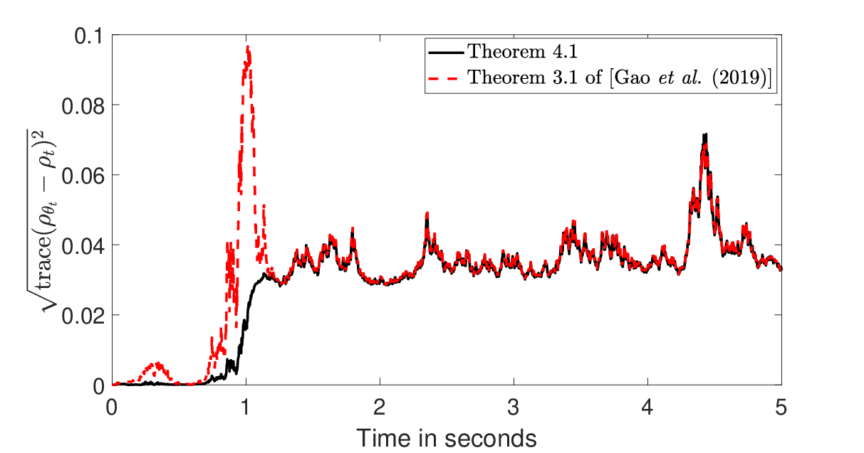
The approximation capability of the quantum projection filter is demonstrated by considering the Hilbert-Schmidt distance between the real quantum state and the normalized state calculated from the quantum projection filter in (5), i.e., . A number of simulations have been conducted and have illustrated the advantages of the proposed approach. Simulation results from one particular experiment are presented in Fig. 1, from which one can observe that the approach in Theorem 4.2 performs better than the one in Theorem 3.1 of [Gao et al. (2019)].
Figure 1: Approximation performance comparison.
6 Conclusions
Based on Stratonovich stochastic Taylor expansions and quantum information geometry techniques, we have provided a new quantum projection filter design. It has been shown by simulation results of a four-level system example that the new quantum projection filter has better approximation capabilities than the existing approach. Future research includes: i) analysis of the approximation errors, especially when the initial quantum state is unavailable; ii) design of more appropriate submanifold for general quantum filter equation and iii) applications of the quantum projection filter to quantum feedback control design.
Appendix
Proof of Theorem 3.1. We provide a proof for the convergence capability of the order Stratonovich stochastic Taylor expansion of as shown in (26). The convergence result in (27) can be derived following a similar procedure and the corresponding proof is omitted.
The proof is decomposed into two steps.
Step 1. We prove
(73)
by induction on the integer . For the case that , the remainder set and (73) becomes
Let be an integer. It follows from the definitions in (11) and (12) that
(75)
Now suppose that (73) holds for the case that . By applying the chain rule in Stratonovich stochastic calculus to the function , one has
(76)
where the third equality in (76) is obtained by applying the formula (73) to the function for , and
(77)
By combining (76) and (77), one obtains that (73) holds for the case . Then by mathematical induction, (73) holds for any nonnegative integer .
Step 2. We prove that the truncation error term in (73) satisfies
(78)
It is noted that . It is also noted that the number of multi-indices belonging to is . Therefore, it is sufficient to prove (78) if we can show that for any
(79)
Now we prove (79) by induction on . For the time interval , we define a partition of time by where the positive integer is chosen to be big enough.
First, consider the case that with . It then follows from the inequality that
(80)
On the other hand, considering the case that with , one has
(81)
Suppose that (79) holds for the case that . Now let with . Then , and . By using the inductive hypothesis, one has
(82)
On the other hand, let . Then , and . By using the inductive assumption, one has
(83)
By combining (82) and (83), one obtains that (79) holds for . One can then conclude that (79) holds for any nonnegative integer by mathematical induction.
References
[Amari & Nagaoka (2000)]
Amari S. & Nagaoka H. (2000).
Methods of Information Geometry.
Oxford: Oxford University Press.
[Armstrong & Brigo (2019)]
Armstrong J. & Brigo D. (2019).
Optimal approximation of SDEs on submanifolds: the -vector and -jet projection.
Proceedings of London Mathemtical Society, 119, 176-213.
[Armstrong & Brigo (2018)]
Armstrong J. & Brigo D. (2018).
Intrinsic stochastic differential equations as jets.
Proceedings of the Royal Society of London A: Mathematical, Physical and Engineering Sciences, 474, http://doi.org/10.1098/rspa.2017.0559.
[Belavkin (1992)]
Belavkin V.P. (1992).
Quantum stochastic calculus and quantum nonlinear filtering.
Journal of Multivariate Analysis, 42, 171-201.
[Bouten et al. (2007)]
Bouten L., van Handel R. & James M. R. (2007).
An introduction to quantum filtering.
SIAM Journal on Control and Optimization, 46, 2199-2241.
[Brigo et al. (1998)]
Brigo D., Hanzon B. & LeGland F. (1998).
A differential geometric approach to nonlinear filtering: the projection filter.
IEEE Transactions on Automatic Control, 43, 247-252.
[Brigo et al. (1999)]
Brigo D., Hanzon B. & LeGland F. (1999).
Approximate filtering by projection on the manifold of exponential densities.
Bernoulli, 5, 495-543.
[Carreo et al. (2017)]
Carreo F., Antn M. A., Yannopapas V. & Paspalakis E. (2017).
Control of the absorption of a four-level quantum system near a plasmonic nanostructure.
Physical Review B, 95, 195410.
[Dong et al. (2019)]
Dong Z., Zhang G. & Amini N. (2019).
Quantum filtering for a two-level atom driven by two
counter-propagating photons.
Quantum Information Processing, 18, 136.
[Emzir et al. (2017)]
Emzir M.F. , Woolley M.J. & Petersen I.R. (2017).
A quantum extended Kalman filter.
Journal of Physics A: Mathematical and Theoretical, 50, 225301.
[Gardiner & Zoller (2000)]
Gardiner C. W. & Zoller P. (2000).
Quantum Noise: A Handbook of Markovian and Non-Markovian Quantum Stochastic Methods with Applications to Quantum Optics. 2nd Edition.
New York: Springer-Verlag.
[Gao et al. (2016)]
Gao Q., Dong D. & Petersen I.R. (2016).
Fault tolerant quantum filtering and fault detection for quantum systems.
Automatica, 71, 125-134.
[Gao et al. (2019)]
Gao Q., Zhang G. & Petersen I.R. (2019).
An exponential quantum projection filter for open quantum systems.
Automatica, 99, 59-68.
[Higham (2001)]
Higham D. (2001).
An algorithmic introduction to numerical simulation of stochastic differential equations.
SIAM Review, 43, 525-546.
[James & Gough (2010)]
James M. R. & Gough J. E. (2010).
Quantum dissipative systems and feedback
control design by interconnection.
IEEE Transactions on Automatic Control, 55, 1806-1821.
[Kloeden & Platen (1999)]
Kloeden P. E., & Platen E. (1999).
Numerical Solution of Stochastic Differential Equations.
Berlin, New York, Springer.
[Lee (2012)]
Lee, J. M. (2012).
Introduction to Smooth Manifolds, 2nd ed.
New York, Springer.
[Nielsen et al. (2009)]
Nielsen A., Hopkins A. & Mabuchi H. (2009).
Quantum filter reduction for measurement-feedback control via unsupervised manifold learning.
New Journal of Physics, 11, 105043.
[Rouchon & Ralph (2015)]
Rouchon P. & Ralph J.F. (2015).
Efficient quantum filtering for quantum feedback control.
Physical Review A, 91, 012118.
[Song et al. (2016)]
Song H., Zhang G. & Xi Z. (2016).
Continuous-mode multi-photon filtering.
SIAM Journal on Control and Optimization, 54, 1602-1632.
[Tsang (2014)]
Tsang M. (2014).
Volterra filters for quantum estimation and detection.
Physical Review A, 92, 062119.
[van Handel & Mabuchi (2005)]
van Handel R. & Mabuchi H. (2005).
Quantum projection filter for a highly nonlinear model in cavity QED.
Journal of Optics B: Quantum and Semiclassical Optics, 7, S226-S236.
[Wiseman & Milburn (2010)]
Wiseman H.M. & Milburn G.J. (2010).
Quantum Measurement and Control.
Cambridge, U.K.: Cambridge University Press.