Parallel Machine Scheduling to Minimize Energy Consumption

Energy is an extremely important and scarce resource, and its consumption is progressively becoming a pivotal concern in modern societies. Computing environments account for a large fraction of the global energy consumption and alarmingly, this fraction is growing at a very high rate [1]. In response to this, modern hardware increasingly incorporates various energy-saving capabilities and scheduling algorithms need to be designed, not only for time and space considerations, but keeping energy consumption in mind as well.

We focus on one of the most common such power-management techniques called a power-down mechanism, which refers to the ability of the processor to transition into a sleep state where it consumes negligible energy. Since “waking-up” the processor requires a certain amount of energy, there is a trade-off to be had between the energy saved by residing in the sleep state and the energy expended in transitioning back to the active state. Intuitively, one should aim to keep the number of transitions to the sleep states low and once in a sleep state remain in it for as long as possible.

Consider a set of jobs with individual release times, deadlines and processing times, that are to be processed on either a single or a multiprocessor system equipped with a powerdown mechanism. The processor consumes one unit of energy per unit of time when in the active state and no energy when in the sleep state. Transitioning from the sleep state to the active state incurs a fixed energy cost. Preemption and migration of jobs is allowed but no job can be simultaneously processed on more than one machine. The goal is to produce a feasible schedule which consumes the minimum energy (or report that no feasible schedule exists). In Graham’s notation, and with $E$ being the appropriate energy function the problems we study can be denoted as $1|r_{j};\overline{d}_{j};\text{pmtn}|E$ and $m|r_{j};\overline{d}_{j};\text{pmtn}|E$ respectively.

The problem on a single machine was first stated in [12], where a greedy $2$-approximation algorithm called Left-To-Right was presented. Roughly speaking, Left-To-Right tries to keep the machine at its current state (active or asleep) for as long as possible. However the computational complexity of the problem remained open and was repeatedly posed as an important open question, in particular because “many seemingly more complicated problems in this area can be essentially reduced to this problem” (c.f. [11]). The complexity question, for the single-machine setting, was eventually settled, initially by Baptiste [6], who gave a $O(n^{7})$-time algorithm for the case of unit-size jobs and subsequently by Baptiste et. al. [7] who achieved a running time of $O(n^{4})$ for unit sized jobs and $O(n^{5})$ when jobs can have arbitrary processing times. Both algorithms are based on a rather involved dynamic programming approach.

The multiprocessor case turns out to be much more challenging than the single processor one, and obtaining any algorithm for it with a non-trivial performance guarantee has been a major open problem [7]. It is also an open problem whether the problem is NP-hard. The difficulty in obtaining a good approximation algorithm seems to arise from two aspects: First, it is not clear how to design a dynamic programming table of polynomial size when the jobs have arbitrary sizes, and a job is not allowed to run parallel to itself. Secondly, structural properties of an optimal schedule can be locally extracted in a single machine environment in contrast to the multi-machine case. As an example, we know that a single machine will be active for at least one time-point within the interval between the release time and the deadline of every job, but the number of active machines at such a time-point in the multiprocessor setting could range from just one to all available machines. As a result, there has been only one previous result with for the multiprocessor setting; by Demaine et al. [9] who extended the dynamic program of Baptiste [6] and showed an $O(n^{7}m^{5})$-time algorithm for the special case of unit-size jobs and $m\geq 1$ machines.

We are given a set of jobs $\left\{j_{1},j_{2},\ldots,j_{n}\right\}$; job $j_{i}$ has release time $r_{i}$, deadline $d_{i}$ and processing time $p_{i}$ and we assume that all these quantities are non-negative integers. Let $r_{min}$ and $d_{max}$ be the earliest release time and furthest deadline of any job; it is no loss of generality to assume $r_{min}=0$ and $d_{max}=D$. For $t\in\mathbb{Z}^{+}$, let $[t,t+1]$ denote the $t^{\rm th}$ time-slot. Let $I=[t,t^{\prime}],t,t^{\prime}\in\mathbb{Z}^{+},t<t^{\prime}$ be an interval. The length of $I$, denoted by $\left|I\right|$ is $t^{\prime}-t$. We use $t\in I_{1}$ to denote $a_{1}\leq t\leq b_{1}$.

Two intervals $I_{1}=[a_{1},b_{1}]$ and $I_{2}=[a_{2},b_{2}]$ overlap if there is a $t$ such that $t\in I_{1}$ and $t\in I_{2}$. Thus two intervals which are right next to each other would also be considered overlapping. Intervals which do not overlap are considered disjoint. $I_{1}$ is contained in $I_{2}$, denoted $I_{1}\subseteq I_{2}$, if $a_{1}\leq a_{2}<b_{2}\leq b_{1}$ and it is strictly contained in $I_{2}$, denoted $I_{1}\subset I_{2}$, if $a_{1}<a_{2}<b_{2}<b_{1}$.

At any time-slot, a machine can be in the active or the sleep state. For each time-slot that a machine is in the active state, one unit of power is required whereas no power is consumed in the sleep state. However, $Q$ units of energy (called wake up energy) are expended when the machine transitions from the sleep to the active state. In its active state, the machine can either process a job (in which case we refer to it as being busy) or just be idle. On the other hand the machine cannot perform any processing while in the sleep state. Note that if a machine is not required to do any processing for $L$ consecutive time-slots, then it is advantageous to transition it to the sleep state when $L>Q$ whereas for $L\leq Q$ it is preferable to keep it active but idle.

A machine can process at most one job in any time-slot and a job cannot be processed on more than one machine in a time-slot. However, job preemption and migration are allowed, i.e., processing of a job can be stopped at any time and resumed later on the same or on a different machine. A job $j_{i}$ must be processed for $p_{i}$ time-slots in $[r_{i},d_{i}]$. Any assignment of jobs to machines and time slots satisfying the above conditions is called a (feasible) schedule. We assume that the machine is initially in the sleep state. Therefore, the energy consumed by a schedule is the total length of the intervals during which the machine is active plus $Q$ times the number of intervals in which the machine is active. The objective of the problem is to find a schedule which consumes minimum energy.

We first show how to schedule jobs on a single machine so that the total energy consumption is at most $P$ more than the optimum. For any $[a,b]\subseteq[0,D]$ (recall $D$ is the furthest deadline of any job), let $V(a,b)=\sum_{i:[r_{i},d_{i}]\subseteq[a,b]}p_{i}$ be the total processing time of jobs whose release and deadline are within $[a,b]$. For an instance to be feasible it is necessary that for all $0\leq a<b\leq D$, $V(a,b)\leq b-a$. The Earliest Deadline First (EDF) algorithm for scheduling jobs with release dates and deadlines can also be used to establish the sufficiency of this condition.

Motivated by this necessary and sufficient condition for determining if an instance is feasible, we consider the following Integer Program for minimizing total energy consumed. For $I\subseteq[0,D]$ let $x_{I}$ be a variable which is 1 if the machine becomes active at the start of $I$ and remains so till its end when it transitions back to the sleep state; $x_{I}$ is 0 otherwise. Since the machine uses $Q$ units of energy to wake-up at the start of $I$ and $\left|I\right|$ units to run during this interval, the objective is to minimize $\sum_{I}x_{I}(Q+\mbox{$\left|I\right|$})$. We next discuss the constraints of this IP.

1. 1.

   The intervals in which the machine is active are disjoint and hence for $0\leq t\leq D$, $\sum_{I:t\in I}x_{I}\leq 1$.

2. 2.

   To ensure that jobs can meet release dates and deadlines when scheduled within active intervals we add the constraint that for all $0\leq a<b\leq D$, $V(a,b)\leq\sum_{I}x_{I}\mbox{$\left|I\cap[a,b]\right|$}$.

3. 3.

   For any job $j_{i}$, the machine should be active at some point during $[r_{i},d_{i}]$. Hence
   $\sum_{I:I\cap[r_{i},d_{i}]\neq\varnothing}x_{I}\geq 1$

This gives us the following integer program.

Consider a feasible solution to this IP and let $\mathcal{I}=\mbox{$\left\{I|x_{I}=1\right\}$}$. A time-slot $[t,t+1]$ is active if it is contained in some interval of $\mathcal{I}$.

The above claim implies that an optimum solution to the integer program gives a feasible schedule which minimizes energy. We relax the integrality constraint on $x_{I}$ to $0\leq x_{I}\leq 1$ and solve the resulting linear program. Let $x$ be the optimum fractional solution and let $\mathcal{I}=\mbox{$\left\{I|x_{I}>0\right\}$}$. We will next show that $x$ be decomposed into a convex combination of integer solutions.

Ordering intervals in $\mathcal{I}$: Let $[a,d],[b,c]\in\mathcal{I}$, $[b,c]\subset[a,d]$ and $x_{[a,d]}=x_{[b,c]}=\alpha$. we replace these intervals in $\mathcal{I}$ with intervals $[a,c],[b,d]$ and set $x_{[a,c]}=x_{[b,d]}=\alpha$. Doing so does not make $x$ infeasible nor does it change the objective value. If $\beta=x_{[a,d]}>x_{[b,c]}=\alpha$ then we replace these intervals in $\mathcal{I}$ with three intervals $[a,d],[a,c],[b,d]$ and set $x_{[a,d]}=\beta-\alpha$ and $x_{[a,c]}=x_{[b,d]}=\alpha$. The case when $\beta=x_{[a,d]}<x_{[b,c]}=\alpha$ is handled similarly. We repeat this process whenever an interval in $\mathcal{I}$ strictly contains another interval in $\mathcal{I}$. Finally, order the intervals in $\mathcal{I}$ by their start-times; intervals which have the same start-time are ordered by their end-times. Let $\prec$ denote this total order on intervals of $\mathcal{I}$. Note that since no interval is strictly contained in another, we would get the same ordering if intervals were ordered by their end-times with intervals having the same end-time ordered by their start-times.

Decomposing $x$ into a convex combination of integer solutions: For $I\in\mathcal{I}$ let $s_{I}$ be the fractional part of $\sum_{I^{\prime}\prec I}x_{I^{\prime}}$; thus $0\leq s_{I}<1$. For $k$, $0\leq k<1$ construct $\mathcal{I}_{k}\subseteq\mathcal{I}$ as follows: $I\in\mathcal{I}_{k}$ iff either $s_{I}\leq k<s_{I}+x_{I}$ or $s_{I}\leq k+1<s_{I}+x_{I}$.

Let $0=s_{1}<s_{2}<\cdots<s_{m}<1$ be the distinct values in the set $\left\{s_{I},I\in\mathcal{I}\right\}$; note that $m\leq\mbox{$\left|\mathcal{I}\right|$}$. From our construction of $\mathcal{I}_{k}$ it follows that for all $k\in[s_{j},s_{j+1})$ the set $\mathcal{I}_{k}$ are identical; let $\mathcal{C}_{j}$ denote this set and we assign it a weight $w_{j}=s_{j+1}-s_{j}$ (or $1-s_{m}$ for the border case when $j=m$). By Claim 2, each “solution” $\mathcal{C}_{j},1\leq j\leq m$ is a set of disjoint intervals.

Extending Intervals: Although $\mathcal{C}_{j},1\leq j\leq m$ is a set of disjoint intervals it need not be a feasible solution, i.e. it could be that jobs cannot meet release dates and deadlines if they have to be scheduled within intervals of $\mathcal{C}_{j}$. This is illustrated by the example in Figure 1, the details of which can be found in the Appendix.

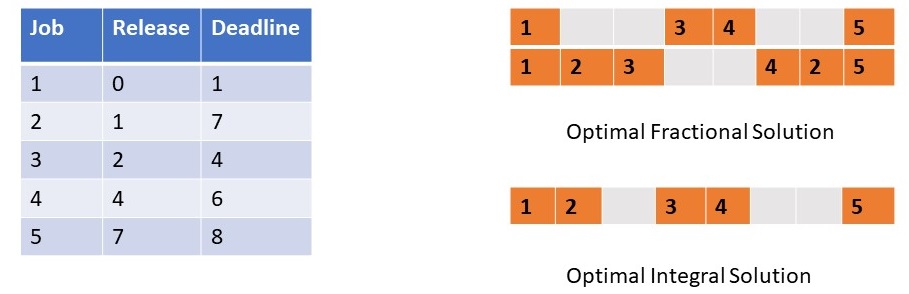
We next show that we can extend the intervals in any solution $\mathcal{C}_{j},1\leq j\leq m$ by at most $P$ units to get a feasible solution, $\mathcal{C}^{\prime}_{j}$.

Since the number of intervals in $\mathcal{C}^{\prime}_{j}$ equals the number of intervals in $\mathcal{C}_{j}$ and the total length of intervals in $\mathcal{C}^{\prime}_{j}$ exceeds the total length of intervals in $\mathcal{C}_{j}$ by at most $P$, the energy consumed by the solution $\mathcal{C}^{\prime}_{j}$ is at most $P$ more than the energy consumed by $\mathcal{C}_{j}$. Since this is true for all solutions $\mathcal{C}^{\prime}_{j},1\leq j\leq m$, the solution of minimum cost among these has cost at most $P$ more than the optimum fractional solution.

In this section we prove a necessary and sufficient condition for scheduling jobs on $m$ parallel machines so that all release dates and deadlines are met. While this is a standard problem in an undergraduate Algorithms course we repeat the argument here since it will be useful in developing the linear program for minimizing energy consumption in the next section.

Recall we are given $n$ jobs. Job $j_{i},1\leq i\leq n$ requires $p_{i}$ units of processing, is released at time $r_{i}$ and has deadline $d_{i}$. The jobs are to be scheduled on $m$ identical machines and we allow for preemption and migration. An instance is feasible iff for every job $j_{i},1\leq i\leq n$ we can assign $p_{i}$ distinct time-slots during $[r_{i},d_{i}]$ such that no time-slot is assigned to more than $m$ jobs.

For reasons that will become clear later, we consider a minor generalization of the above problem which we refer to as deadline-scheduling-on-intervals. Instead of $m$ machines, we are given $k$ supply-intervals, $\mathcal{I}=\mbox{$\left\{I_{1},I_{2},\ldots,I_{k}\right\}$}$ and are required to schedule the given jobs within these intervals. Let $s_{j},t_{j}$ denote the start and end-times of interval $I_{j}$. The intervals in $\mathcal{I}$ need not be disjoint; however any point in time is contained in at most $m$ intervals. Note that if each interval in $\mathcal{I}$ was $[0,D]$ then we would recover the problem of scheduling on parallel machines. An instance of this problem is thus specified by the processing time, release date and deadline of each of the $n$ jobs and the start and end-times of the $k$ supply-intervals. The feasibility of an instance can be checked by formulating it as a problem of finding a flow in a suitable network.

Construct a network $G=(V,E)$ with source $s$, sink $t$, a vertex $u_{i}$ for each job $j_{i}$ and a vertex $v_{t}$ for each time-slot $[t,t+1],0\leq t\leq D-1$. Vertex $u_{i}$ has edges to vertices $\left\{v_{t}|[t,t+1]\subseteq[r_{i},d_{i}]\right\}$ of capacity 1 and an edge from $s$ of capacity $p_{i}$. Let $m_{t}$ be the number of intervals in $\mathcal{I}$ which contain the time-slot $[t,t+1]$. Vertex $v_{t}$ has an edge to the sink $t$ of capacity $m_{t}$. Let $c:E\rightarrow\mathbb{R}^{+}$ denote the capacity function on the edges.

The $s$-$t$ cut $(\mbox{$\left\{s\right\}$},V-\mbox{$\left\{s\right\}$})$ has capacity $P=\sum_{j=1}^{n}p_{j}$ and so the maximum flow between $s$ and $t$ cannot exceed $P$.

Let $(S,\overline{S})$ be an $s$-$t$ cut and $c(S)$ denote its capacity.

We aggregate the time-slots corresponding to vertices in $S\cap\mbox{$\left\{v_{0},v_{1},\ldots,v_{D-1}\right\}$}$ into a minimal set of intervals, $Q(S)$. No two intervals in $Q(S)$ are overlapping since we could combine them and obtain a smaller set of intervals. Recall that if two intervals share an end-point then we consider them overlapping.

If $I_{1},I_{2}$ are disjoint intervals then $\mbox{\tt fv($j_{i},I_{1}$)}+\mbox{\tt fv($j_{i},I_{2}$)}\leq\mbox{\tt fv($j_{i},I_{1}\cup I_{2}$)}$. For instance suppose $I_{1}=[0,3]$, $I_{2}=[5,8]$, $r_{1}=2$, $d_{1}=6$ and $p_{1}=3$. Then fv($j_{1},I_{1}$)=fv($j_{1},I_{2}$)=0 but fv($j_{1},I_{1}\cup I_{2}$)=1. Note that the forced volume of a job $j_{i}$ with respect to an interval $[a,b]$ is independent of the supply-intervals and depends only $a,b,p_{i},r_{i}$ and $d_{i}$. For instance, if $r_{i}<a<d_{i}<b$ then $\mbox{\tt fv($j_{i},[a,b]$)}=\max(0,r_{i}+p_{i}-a)$. Similarly, if $r_{i}\leq a<b\leq d_{i}$ then $\mbox{\tt fv($j_{i},[a,b]$)}=\max(0,p_{i}-(a-r_{i})-(d_{i}-b))$.

Note that deficiency of $Q$ also depends on the supply intervals in the instance. From the above definition it follows that if a set of disjoint intervals, $Q$, has positive deficiency then the instance is infeasible. The following lemma will help us argue the converse.

By Lemma 2 an infeasible instance has a cut $(S,\overline{S})$ such that $c(S)<P$. Lemma 3 then implies that $\mbox{\tt def($Q(S)$)}>0$ which proves the following theorem.

Making an instance feasible: Given an infeasible instance of deadline-scheduling-on-intervals, we would like to extend the intervals of the instance to make it feasible. We need some additional tools to do this and shall take this up in a later section. Let $F<P$ be the maximum $s$-$t$ flow in the network $G$ corresponding to this instance. We now show that an $s$-$t$ flow of value $P$ can be routed in $G$ by increasing capacities of edges incident to the sink such that the total increase in capacities is $P-F$.

By submodularity of the cut-function it follows that if $(S_{1},\overline{S_{1}})$,$(S_{2},\overline{S_{2}})$ are minimum $s$-$t$ cuts then $(S_{1}\cap S_{2},\overline{S_{1}\cap S_{2}})$ is also a minimum $s$-$t$ cut. Hence a minimum $s$-$t$ cut in which the side containing the source is minimal is unique; let $(S,\overline{S})$ be this cut. Since the capacity of this cut is less than $P$, by Claim 5 it follows that $S\cap\mbox{$\left\{v_{0},v_{1},\ldots,v_{D-1}\right\}$}\neq\varnothing$.

Claim 6 gives us an algorithm for increasing capacities. At each step we find a minimum $s$-$t$ cut in which the side containing the source is minimal and increase the capacity of any edge in this cut which is also incident to the sink by 1. Since with every step, we increase the $s$-$t$ flow in $G$ by 1, the number of steps, and the total increase in edge capacities, equals $P-F$.

Claim 6 also implies that $(S,\overline{S})$ remains a minimum $s$-$t$ cut in $G$ even after we increase the capacity of edge $(v_{i},t),v_{i}\in S$, by 1; however $S$ need not be minimal. Let $(S^{\prime},\overline{S^{\prime}})$ be the new $s$-$t$ minimum cut in which the side containing the source is minimal. The fact that $(S,\overline{S})$ is a minimum $s$-$t$ cut implies that $S^{\prime}\subseteq S$. Thus with every step the $s$-side of the cut under consideration shrinks. This is an important property of this process and shall find use later.

We are now ready to give a linear programming relaxation for the problem of scheduling jobs on parallel machines so as to minimize total energy consumed. A solution to the problem is completely specified by the set of time intervals in which each machine is active; let $\mathcal{I}$ be this multiset. The energy consumed by this solution equals $\sum_{I\in\mathcal{I}}(\mbox{$\left|I\right|$}+Q)$. Note that at most $m$ intervals in $\mathcal{I}$ can overlap at any point in time. Further, $\mathcal{I}$ forms a feasible solution if the corresponding instance of deadline-scheduling-on-intervals is feasible.

With every interval $I\subseteq[0,D]$ we associate a variable $x(I),0\leq x(I)\leq m$ which indicates the number of times $I$ is picked in a solution. The objective is to minimize $\sum_{I}x(I)(\mbox{$\left|I\right|$}+Q)$. We now list the constraints of this linear program.

1. 1.

   Let $m_{t}=\sum_{I:[t,t+1]\subseteq I}x(I)$. Since at most $m$ intervals overlap at any time $t$ we get that for all $t,0\leq t\leq D-1$, $m_{t}\leq m$.

2. 2.

   Let $f(i,t)$ be a variable denoting the flow in the edge $(u_{i},v_{t}),0\leq i\leq n,0\leq t\leq D-1$ in the flow network $G$ corresponding to this instance. Then $0\leq f(i,t)\leq 1$.

3. 3.

   The conservation constraint on vertex $v_{t}$ and the capacity constraint on edge $(v_{t},t)$ together give: for all $t,0\leq t\leq D-1$, $\sum_{i:[t,t+1]\subseteq[r_{i},d_{i}]}f(i,t)\leq m_{t}$.

4. 4.

   Since $P$ units of flow have to be routed, all edges incident to the source are saturated. This together with the conservation constraint at vertex $u_{i}$ yields: for all $i$, $\sum_{t=r_{i}}^{d_{i}-1}f(i,t)=p_{i}$.

5. 5.

   Consider an interval $[a,b]\subseteq[0,D]$. The total forced volume of all jobs with respect to $[a,b]$ equals $\sum_{i=1}^{n}\mbox{\tt fv($j_{i},[a,b]$)}$. If this quantity equals $\alpha(b-a)$ then the number of intervals overlapping $[a,b]$ should be at least $\lceil\alpha\rceil$. This yields the constraint: for all $0\leq a<b\leq D$,

   $$\sum_{I:[a,b]\cap I\neq\varnothing}x_{I}\geq\bigg\lceil\frac{\sum_{i=1}^{n}\mbox{\tt fv($j_{i},[a,b]$)}}{b-a}\bigg\rceil.$$

Thus our linear program for scheduling on multiple machines to minimize energy is as follows.

Our algorithm for the case of parallel machines is along the lines of the one for single machines. We begin by solving the linear program from Section 5 and let $x$ be the optimum fractional solution and OPT the cost of this solution. Our algorithm will produce a solution of cost at most $2\mbox{\tt OPT}+P$.

Let $\mathcal{I}=\mbox{$\left\{I|x_{I}>0\right\}$}$. After ensuring that no interval of $\mathcal{I}$ is strictly contained in another, we order the intervals by increasing start-times (breaking ties using end-times) and let $\prec$ be this order. As in Section 3, we construct $r$ integral solutions, $\mathcal{C}_{i},1\leq i\leq r$ and associate weights $w_{i}$ with solutions $\mathcal{C}_{i}$ such that this forms a convex decomposition of $x$. Note that $\mathcal{C}_{i}$ is no more a disjoint set of intervals as in the single machine case. However at most $m$ intervals of $\mathcal{C}_{i}$ could overlap at any point in time.

For the rest of this section we will consider one of the integral solutions in the convex decomposition and refer to it as $\mathcal{C}$. The arguments of this section will apply to all $r$ solutions. Note that $\mathcal{C}$ need not be a feasible instance of deadline-scheduling-on-intervals and we will modify the intervals in $\mathcal{C}$ to make it a feasible solution. Let $I_{1}\prec I_{2}\prec\cdots\prec I_{N}$ be the intervals in $\mathcal{C}$.

Modifying intervals: Let $s_{j},e_{j}$ denote the start and end times of interval $I_{j}\in\mathcal{C}$. We consider the intervals in the order $\prec$ and modify them as follows:

If $I_{j},I_{j+1}$ overlap then replace $I_{j}$ with the interval $[s_{j},e_{j+1}]$. Else create a copy of $I_{j+1}$ if it does not overlap $I_{j+m}$.

For $j=0$ we add a copy of $I_{1}$ if it does not overlap $I_{m}$. The set of intervals formed through this modification continue to have the property that no interval is strictly contained in another although now we could have two copies of some intervals. Let $I^{\prime}_{1}\prec I^{\prime}_{2}\prec\cdots\prec I^{\prime}_{M}$ be the new (multi)set of intervals which we denote by $\mathcal{C}^{\prime}$.

References

- [1] How Dirty is your Data? https://www.greenpeace.org/international/publication/7196/how-dirty-is-your-data/, 2011.
- [2] Susanne Albers. On energy conservation in data centers. In Proceedings of the 29th ACM Symposium on Parallelism in Algorithms and Architectures, SPAA 2017, Washington DC, USA, July 24-26, 2017, pages 35–44, 2017.
- [3] Susanne Albers and Antonios Antoniadis. Race to idle: New algorithms for speed scaling with a sleep state. ACM Trans. Algorithms, 10(2):9:1–9:31, 2014.
- [4] Antonios Antoniadis, Chien-Chung Huang, and Sebastian Ott. A fully polynomial-time approximation scheme for speed scaling with sleep state. In Proceedings of the Twenty-Sixth Annual ACM-SIAM Symposium on Discrete Algorithms, SODA 2015, San Diego, CA, USA, January 4-6, 2015, pages 1102–1113, 2015.
- [5] John Augustine, Sandy Irani, and Chaitanya Swamy. Optimal power-down strategies. SIAM J. Comput., 37(5):1499–1516, 2008.
- [6] Philippe Baptiste. Scheduling unit tasks to minimize the number of idle periods: a polynomial time algorithm for offline dynamic power management. In Proceedings of the seventeenth annual ACM-SIAM symposium on Discrete algorithm, pages 364–367. Society for Industrial and Applied Mathematics, 2006.
- [7] Philippe Baptiste, Marek Chrobak, and Christoph Dürr. Polynomial time algorithms for minimum energy scheduling. In European Symposium on Algorithms, pages 136–150. Springer, 2007.
- [8] Marek Chrobak, Uriel Feige, Mohammad Taghi Hajiaghayi, Sanjeev Khanna, Fei Li, and Seffi Naor. A greedy approximation algorithm for minimum-gap scheduling. Journal of Scheduling, 20(3):279–292, 2017.
- [9] Erik D Demaine, Mohammad Ghodsi, Mohammad Taghi Hajiaghayi, Amin S Sayedi-Roshkhar, and Morteza Zadimoghaddam. Scheduling to minimize gaps and power consumption. In Proceedings of the nineteenth annual ACM symposium on Parallel algorithms and architectures, pages 46–54. ACM, 2007.
- [10] Erik D. Demaine and Morteza Zadimoghaddam. Scheduling to minimize power consumption using submodular functions. In SPAA 2010: Proceedings of the 22nd Annual ACM Symposium on Parallelism in Algorithms and Architectures, Thira, Santorini, Greece, June 13-15, 2010, pages 21–29, 2010.
- [11] Sandy Irani and Kirk Pruhs. Algorithmic problems in power management. SIGACT News, 36(2):63–76, 2005.
- [12] Sandy Irani, Sandeep K. Shukla, and Rajesh Gupta. Algorithms for power savings. ACM Trans. Algorithms, 3(4):41, 2007.
- [13] Sandy Irani, Sandeep K. Shukla, and Rajesh K. Gupta. Online strategies for dynamic power management in systems with multiple power-saving states. ACM Trans. Embedded Comput. Syst., 2(3):325–346, 2003.
- [14] Gunjan Kumar and Saswata Shannigrahi. On the NP-hardness of speed scaling with sleep state. Theor. Comput. Sci., 600:1–10, 2015.
Appendix
Appendix A From Pseudopolynomial to Polynomial Time
In this section we prove that it is sufficient to limit ourselves to intervals with start and endpoints from a set of polynomially many time-slots in , with the loss of a small factor in the approximation ratio.
Definition 3.
Let and .
Claim 8.
is polynomial in the input size, and therefore so is the number of possible intervals that start and end at time-slots of .
Proof.
Consider some . We argue about the number of distinct , so that for some . Since , we have that and therefore . In turn , and the number of possible intervals starting and ending at is . ∎
Lemma 6.
Considering only intervals that start and end at time-slots of W, does not increase the cost of being in the active state by more than a factor of .
Consider an optimal solution OPT. We will transform OPT to a solution that satisfies the lemma property while increasing its active cost by at most an factor. We can associate intervals in OPT with processors as follows. Recall that the intervals are ordered by their start-time and ties are broken by end-times. Go through the intervals in this order and associate each interval to the smallest-index processor so that it does not overlap with any other interval already there. We will use the following claim to prove the lemma:
Claim 9.
Assuming that holds for any interval is without loss of generality.
Consider some interval , associated with a processor and let be a time slot of whose existence is guaranteed by Claim 9.
We will expand towards the left and the right respectively until we hit either some time slot in or we hit another interval associated with this processor. In the second case we merge the two intervals. We repeat this for every interval, and the process will terminate since in each step we either ”snap” one of the endpoints to a point in or reduce the number of intervals by one. Note that eventually all interval endpoints will be slots in ( includes and ).
The total increase in length of an interval is at most , because we expand towards the left by at most a factor , and similarly towards the right by at most a factor . This is because by construction there are points in at every multiple distance away from , and we never expand more than that.
We conclude the proof of the lemma by proving Claim 9.
Proof of Claim 9.
Assume for the sake of contradiction that there exists an such that . Then we move towards an adjacent point . Without loss of generality assume that we move leftwards. So consider moving leftwards one slot at a time. We break up this moving of one slot leftwards into consecutively moving all units of one slot leftwards: We first move the leftmost unit, then the next one etc. The following could potentially happen:
- •
Interval reaches . In this case and we stop.
Interval meets the endpoint of some other interval on the same or a different processor. This cannot happen since it would contradict the optimality of OPT. The reason is that one can either merge with , or use part of to close the gap following on its processor. Either requires one wake-up operation less but has otherwise identical costs to OPT.
We are not able to move some unit of one more slot leftwards without producing an infeasible schedule. Since there is still no point in intersecting this must be because some job running in this unit of would run in parallel to itself if we move the interval one more slot leftwards. Let be the slot on which runs in , and assume that it runs in some slot on some other processor. If there is some interval on one of the other processors ending at slot , we simply move the unit of to that processor continue shifting the remaining slots of to the left. Thus we may assume that slot contains strictly less jobs than slot . By the pigeon hole principle there exists some job that we can swap with in slot so that we can move one more unit of one slot leftwards.
Since in each step we move one unit of one slot leftwards, the process will eventually terminate with . Note that the process does not increase the number of intervals, nor the sum of interval lengths (although it may change individual interval lengths), and therefore does not affect the cost of the solution. ∎
∎
Modifying the Flow Network and Linear Program. We first show how to modify the network for checking the feasibility of deadline-scheduling-on-intervals. Let , with . The consecutive points in partition into time intervals, ie. . We refer to the interval as the time slot. We next discuss how to adapt the maximum flow formulation. Firstly, instead of nodes for each time , we now have a node for each time slot in . The capacity of edge is the length of interval . Let be the number of intervals crossing time slot . The capacity of edge is , where is defined as the product of and the length of time slot . Note that size of the network after doing the above modification is . As in Lemma 2, we can again argue that the given instance is feasible iff units of flow can be routed in the network. If the instance is feasible, then units of flow can clearly be routed. Suppose units of flow can be routed in the network. Fix a time slot . We have to schedule units of job in the time slot such that and . Consider a schedule of all jobs (active in time slot ) on a single machine such that job is processed for units, every job is processed contiguously and there is no gap in the schedule. The machine runs continuously in . We replicate the schedule of this machine in time on the interval crossing time slot . No job is processed in two intervals at the same time as no job has length more than . We modify appropriate constraints in the Linear Program to reflect changes made in the network.
Modifying the Rounding Procedure. We now argue that the rounding procedure of Section 6 can be carried out in polynomial time. The algorithm works in iterations. In each iteration, the rounding procedure finds a minimal set of intervals of maximum deficiency and increases the length of an interval in this set by 1. This results in reduction of maximum deficiency by 1 and there can be at most such iterations. We make the following minor modification to this algorithm. If we decide to extend an interval of some solution in an iteration, we extend it by , where is the maximum number such that extending by also reduces the maximum deficiency of this solution by . We can find such a by binary search. Recall that minimal maximum deficiency set shrinks after every iteration. Suppose is the minimal maximum deficiency set after was extended by . Since was not extended any further (in a previous iteration), either it does not overlap with or none of the endpoints of are inside . In either case, this interval will never be extended in any further iteration. Hence, the total number of iterations is bounded by the maximum number of intervals in a solution, which is . Since total number of solutions is at most the number of possible intervals, the total number of iterations required for constructing all the solutions is at most . Also, the total length of intervals added to a solution is equal to the maximum deficiency, which is at most and hence the rounding procedure does not further affect the approximation guarantee of the algorithm. After extending the intervals, each solution has a maximum deficiency of zero and hence feasible (by discussion in the last section).
Appendix B Integrality Gap Example
Consider an instance on a single machine with 5 jobs, (see Figure 1). Let . All jobs have unit processing time and the wake up cost of the machine is . Since the wake up cost is we may assume that the machine transitions to the sleep state whenever it is idle, in other words there exists an optimal (integral) solution with no active but idle periods. We claim that the aforementioned instance requires at least three contiguous active time intervals: First note that and have to be done in time slots and respectively and since there are only three units of work to be done in , and must be processed in two different intervals. Let and be these respective intervals. If is processed in , then cannot be processed in or . Similarly, if is processed in , then cannot be processed in or . Hence, optimal solution must incur wake up energy of at least and total energy of optimal solution is at least .
We now show a fractional solution with value strictly smaller than 8. Let (see Figure 1). Consider a fractional solution with . It can easily be verified that this is a feasible fractional solution with energy 15/2. Hence, integrality gap of the LP is at least .