On Occupation Time for On-Off Processes with Multiple Off-StatesThanks:
1. Department of Statistics, University of Connecticut, 215 Glenbrook Road, Storrs, CT 06269-4120
* Corresponding author. E-mail: chaoran.hu@uconn.edu
Abstract.
The need to model a Markov renewal on-off process with multiple off-states arise in many applications such as economics, physics, and engineering. Characterization of the occupation time of one specific off-state marginally or two off-states jointly is crucial to understanding such processes. We derive the exact marginal and joint distributions of the off-state occupation times. The theoretical results are confirmed numerically in a simulation study. A special case when all holding times have Lévy distribution is considered for the possibility of simplification of the formulas.
Keywords: Lévy distribution, Markov renewal process, Telegraph process
1. Introduction
Markov renewal on-off processes, also known as alternating renewal processes or telegraph processes, arise in applications in a variety of fields. Classic alternating renewal processes were first studied by Cane 1959, Page 1960 and Newman 1968 with appxlications to animal ethology, maintenance of electronic equipment, and communication engineering, respectively. Recently, the telegraph process and their variations are employed in various fields of applications such as pricing in mathematical finance and insurance [9, 6, 7, 8, 16, e.g.,], modelling the propagation of a damped wave in physics [4, 10, e.g.,], and inventory and storage models in engineering [18]. In certain applications, the off-state of an on-off process has multiple types, which raises new questions about its properties such as the distribution of the occupation time in specific off-state type marginally or multiple off-state types jointly. Our interest in on-off processes with multiple off-states is motivated by our recent work in animal movement modeling, where a predator can have different non-moving states such as resting or handling a kill [15, 14]. The occupation time in the handling state is important for ecologists to understand the behavior of predators.
To fix ideas, consider a server that has two different types of failures, each requiring a different time and cost to repair. One basic question is: if the server is on at time 0, what is the distribution of the time one spends fixing the type one failures by time ? We model the server state process with the following Markov renewal process. The process starts in state 0 (the on-state) and spend there a random holding time according to a given absolutely continuous distribution. When the first holding time is over, we flip an asymmetric coin to decide which type of failure (off-state 1 or off-state 2) comes next. The holding times in the off-states are also absolutely continuous, generally with different distributions. Once the second holding time is over the process returns to the on-state (state 0) and then we repeat the construction process.
The occupation time of a specific type of the off-state is our focus. For the on-state, the distribution of the occupation time is known from the results on the telegraph process [13, 5, 17, 19]. Indeed, if we collapse the two off-states into one, then the resulting process is a regular on-off process (or alternating renewal process) whose off-state holding time distribution is a mixture of the two original off-state holding time distributions. If the different types of repair require different resources, however, we want to know the distribution of the occupation time in a particular type of off-state. For that task, the results on classical telegraph processes are not directly applicable. Moreover, assume that the cost for being in an off-state is proportional to its occupation time and different for different off-states. If one wants to know the distribution of the total cost for repairs of all kinds by a fixed time, then we need the joint distribution of the two types of off-state occupation times.
Our problem is related to but different from some recent works. An extension of the telegraph process to a process with three states is studied in Bshouty et al. 2012, where within a renewal cycle all three states are visited in a given deterministic order. In our case, however, we have an on-off process with two off-states; only two states (the on-state and an off-state) are visited in each renewal cycle, but the off-states is chosen randomly. Another related work is Crimaldi et al. 2013, where there are two states, but at each random epoch, the new state is determined by the outcome of a random trial, and, as a result, the process can stay in the same state.
The key idea to study the occupation time of a specific off-state is to exploit a certain periodicity of our Markov renewal process. In fact, when analyzing any Markov renewal process, it is always convenient to do the conditioning on returning to a certain state. For the on-off process with two off-states, state 0 has an additional nice property. The numbers of steps between two consecutive visits of state 0 is not random, and it is always equal to 2. We derive the marginal distribution of the occupation time of a specific off-state first, and then we modify our derivation to obtain the joint distribution of the two off-state occupation times. Of course, one can get the marginal distribution by integrating the joint one. Our approach, however, is easier to follow.
2. Algorithmic Construction of On-Off Process with Two Off-States
Suppose that we are given the following collection of independent sequences of non-negative random variables:
- (1)
are independent identically distributed (iid) random variables with cumulative distribution function (cdf) and probability density function (pdf) (these random variables will be used as the holding times when the server is up, state 0);
- (2)
are iid random variables with cdf and pdf (holding times when the server is down for short repairs, state 1);
- (3)
are iid random variables with cdf and pdf (holding times when the server is down for long repairs, state 2);
- (4)
are iid random variables with and .
Now, we present our construction of the on-off process with two off-states, .
- (1)
Initialize with and .
- (2)
For cycles :
- (a)
Let , and for all .
- (b)
If then , and for all ; otherwise, , and for all .
- (a)
Then the occupation times in state 0, state 1, and state 2 are, respectively,
The corresponding defective marginal densities of and are denoted as
where , , . The defective joint two-dimensional density of and for , is denoted as
where . The densities are defective in the following sense: since both occupation times and have an atom at 0, all three sums
and
are less than 1.
3. Marginal Distribution of Occupation Time of an Off-State
To derive the distribution of occupation time we will need some auxiliary random variables. Let be the number of cycles (or returns to the on-state) by time . Formally, for
Finally, let . These random variables are associated with the off-state holding time of the regular on-off process when two off-states are combined.
Our formulas include convolutions of different distributions. We will use the following notation. If we are given a cdf and its pdf , then denotes -fold convolution of , and denotes the -fold convolution of . If we are given two cdfs and with pdfs and , then denotes the convolution of cdfs and , and denotes the convolution of pdfs and .
We also use the following conventions. Any summation over the empty set is 0. Zero-fold convolution is the cdf of a random variable that is equal to 0 with probability 1. Finally, for any .
Theorem 1.
Let and . Then
and
Proof.
First, note that the distribution of has an atom. Indeed, if or all the failures that occur before are of the second type, then . More specifically, by conditioning on the number of returns to the on-state, , we obtain that
Next, again by conditioning on , we get that for
Note that the summation starts from 1, because and implies that , and, therefore, .
The next step is to fix the number of switches to failures of type 1. Since the total numbers of switches is and there is at least one failure of type 1, we have
Because
and it really does not matter during which cycles the switches to failures of type 1 occur, we find that
Next, observe that in this case . Using independence between and the holding time sequences we have
Finally, independence of holding time sequences gives us that
Now let us consider the case when (at time the server is down for a short repair). One difference is that there is no atom in this case. As before, for we have
Note that event
can be rewritten as
Since , we finally obtain
The other formulas can be derived in a similar way. ∎
4. Joint Distribution of Off-State Occupation Times
As mentioned in the introduction, if we are interested in the distribution of the total cost, then we need the joint distribution of off-state occupation times. More specifically, assume that the total cost is a linear function of occupation times, that is,
Then the distribution of is fully determined by the joint distribution of and . Note that we do not need the joint distribution of all three occupation times, because .
Since both and have atoms at 0, for every value of we have four cases: (1) both occupation times are 0; (2) , ; (3) , ; and (4) both and are strictly greater than 0. In total, we have 12 formulas. Some of them are trivial. For instance, event has probability 0, therefore, the corresponding defective one-dimensional density of is also 0. Moreover, since there is a certain symmetry between and some formulas can be found by interchanging state 1 and 2. That is why in the following theorem below we have only 5 formulas.
Theorem 2.
Let and . Then
and
Proof.
We will only derive the formula for . The remaining formulas can be obtained by similar modifications of the proof of Theorem 1.
As before, we start with partitioning with respect to events . More specifically, for and we have
Note that now the upper limit of the inner summation is , because and implies that .
Next, observe that event
can be rewritten as
Finally, taking into account that in the case when occupation time and occupation time , we get that
∎
One can verify now that, for instance,
Using symmetry between and , we also can get that
5. Special Case: Lévy Distribution
In this section we consider a special case when all the holding times have the Lévy distribution (with location parameter 0 and possibly different scale parameters). The Lévy distribution with scale parameter has pdf
and cdf
The Lévy distribution is heavy-tailed with infinite expectation. The median is given by , where is the complementary error function:

The parametrization that we use is a bit unusual, but it allows us to shorten our notation for convolutions. More specifically, as a member of the family of stable distributions with mobility parameter 1/2, the Lévy distribution is closed under the operation of convolution in the following way:
Let , , and be the scale parameters for states 0, 1 and 2, respectively. Then the formulas from Theorem 1 and Theorem 2 do not involve any convolutions. For instance, in this case we have that
The expectations and variances of the off times is given by
Note that the discrete component of the occupation times is not used for these calculations, because the atoms are at 0. The covariance of and is given by
As an example we consider a server with median holding time 7 days, 0.5 hour, and 4 hours for the on-state, the short off-state, and the long off-state, respectively. Using one day as the time unit, the model parameters are: , , and . Assume also that the total repair cost is given by
that is, long repairs are twice costlier than the short ones.
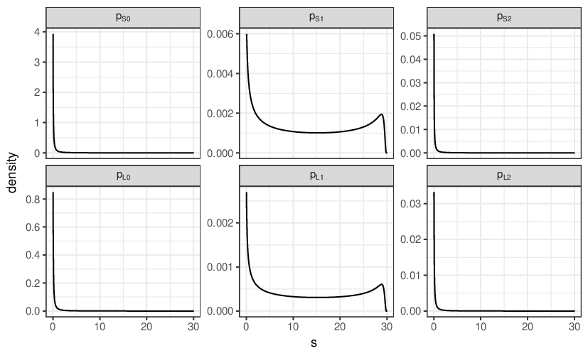
Figure 1 presents defective marginal densities and when days and (that is, the less serious breakdowns occur 9 times more often). The marginal densities for both occupation times are severely defected when (the process is in the on-state). As we mentioned above and have atoms at :
Figure 2 shows the contour plot of defective joint densities with the same parameter setup, where the negative association of the two occupation times is obvious. We also ran a simulation study to numerically confirm the correctness of Theorem 1 and Theorem 2. A total realizations of the above on-off process were generated and the empirical results are consistent with the theoretical densities (not shown).
Table 1 summarizes the expectation and variance of the two types of off-state occupation times and the associated repair cost for days and . As increases, the expectation and the variance goes up for the less serious breakdown time but goes down fro the more serious breakdown time. The total repair cost has lower expectation and variance for smaller values of . The correlation of the two off-state occupation times is negative, with a magnitude decreasing as increases. When is doubled, the expectation of the occupation times and the total repair cost is slightly more than doubled, which is because the process always starts from the on-state with a random holding time.
| 30 | 0.70 | 0.81 | 10.82 | 0.95 | 13.01 | 2.71 | 60.99 | 0.040 |
| 0.75 | 0.87 | 11.60 | 0.79 | 10.95 | 2.46 | 53.71 | 0.037 | |
| 0.80 | 0.93 | 12.38 | 0.64 | 8.85 | 2.20 | 46.32 | 0.035 | |
| 0.85 | 0.99 | 13.15 | 0.48 | 6.70 | 1.95 | 38.80 | 0.031 | |
| 0.90 | 1.05 | 13.93 | 0.32 | 4.51 | 1.69 | 31.16 | 0.026 | |
| 0.95 | 1.11 | 14.70 | 0.16 | 2.28 | 1.43 | 23.38 | 0.019 | |
| 0.99 | 1.16 | 15.32 | 0.03 | 0.46 | 1.23 | 17.07 | 0.009 | |
| 60 | 0.70 | 1.75 | 48.20 | 2.08 | 57.96 | 5.92 | 271.58 | 0.040 |
| 0.75 | 1.88 | 51.68 | 1.74 | 48.81 | 5.37 | 239.32 | 0.038 | |
| 0.80 | 2.02 | 55.16 | 1.40 | 39.46 | 4.82 | 206.48 | 0.035 | |
| 0.85 | 2.15 | 58.64 | 1.05 | 29.91 | 4.26 | 173.04 | 0.031 | |
| 0.90 | 2.29 | 62.13 | 0.70 | 20.16 | 3.70 | 139.01 | 0.026 | |
| 0.95 | 2.42 | 65.62 | 0.35 | 10.19 | 3.13 | 104.37 | 0.019 | |
| 0.99 | 2.53 | 68.41 | 0.07 | 2.05 | 2.67 | 76.21 | 0.009 |
6. Concluding Remarks
The obtained results can be generalized to the case of more than two off-states. The only difference is that instead of binomial probabilities one has to use multinomial ones.
The marginal distribution of an off-state occupation time could be obtained by collapsing the on-state with the other off-state and using results on the telegraph process. Nonetheless, this approach would lead to more complicated formulas because the holding time of the new collapsed state is distributed as an infinite mixture of convolutions. And of course, this technique cannot be employed if we need the joint distribution of the two off-state occupation times.
The process also can be viewed as a telegraph process governed by the on-off process with multiple off-states. That is, is the time position of a particle that moves with speed whenever (). The formulas for the joint distribution of and occupation times can be useful for parameter estimation when process is discretely observed. In particular, if is also Markov (that is, all the holding times are exponential) then the efficient likelihood estimation is possible with help of tools for hidden Markov model [14].
References
- Bshouty et al. [2012] D. Bshouty, A. Di Crescenzo, B. Martinucci and S. Zacks (2012). “Generalized telegraph process with random delays.” Journal of Applied Probability 49, 850–865.
- Cane [1959] V. R. Cane (1959). “Behavior sequences as semi-Markov chains.” Journal of the Royal Statistical Society, Series B 21, 36–58.
- Crimaldi et al. [2013] I. Crimaldi, A. Di Crescenzo, A. Iuliano and B. Martinucci (2013). “A generalized telegraph process with velocity driven by random trials.” Advances in Applied Probability 45, 1111–1136.
- De Gregorio and Macci [2012] A. De Gregorio and C. Macci (2012). “Large deviation principles for telegraph processes.” Statistics & Probability Letters 82, 1874–1882.
- Di Crescenzo [2001] A. Di Crescenzo (2001). “On random motions with velocities alternating at Erlang-distributed random times.” Advances in Applied Probability 33, 690–701.
- Di Crescenzo et al. [2013] A. Di Crescenzo, A. Iuliano, B. Martinucci and S. Zacks (2013). “Generalized telegraph process with random jumps.” Journal of Applied Probability 50, 450–463.
- Di Crescenzo et al. [2014] A. Di Crescenzo, B. Martinucci and S. Zacks (2014). “On the geometric brownian motion with alternating trend.” Mathematical and statistical methods for actuarial sciences and finance, Eds. Perna, C. and Sibillo, M. pp. 81–85.
- Di Crescenzo and Zacks [2015] A. Di Crescenzo and S. Zacks (2015). “Probability law and flow function of Brownian motion driven by a generalized telegraph process.” Methodology and Computing in Applied Probability 17, 761–780.
- Kolesnik and Ratanov [2013] A. D. Kolesnik and N. Ratanov (2013). Telegraph processes and option pricing. Springer Briefs in Statistics. Springer, Heidelberg.
- Macci [2016] C. Macci (2016). “Large deviations for some non-standard telegraph processes.” Statistics & Probability Letters 110, 119–127.
- Newman [1968] D. S. Newman (1968). “On the probability distribution of a filtered random telegraph signal.” The Annals of Mathematical Statistics 39, 890–896.
- Page [1960] E. S. Page (1960). “Theoretical considerations of routine maintenance.” The Computer Journal 2, 199–204.
- Perry et al. [1999] D. Perry, W. Stadje and S. Zacks (1999). “First-exit times for increasing compound processes.” Communications in Statistics: Stochastic Models 15, 977–992.
- Pozdnyakov et al. [2018] V. Pozdnyakov, L. Elbroch, C. Hu, T. Meyer and J. Yan (2018). “On estimation for Brownian motion governed by telegraph process with multiple off states.” ArXiv e-prints .
- Pozdnyakov et al. [2017] V. Pozdnyakov, L. Elbroch, A. Labarga, T. Meyer and J. Yan (2017). “Discretely observed Brownian motion governed by telegraph process: estimation.” Methodology and Computing in Applied Probability to appear.
- Ratanov [2017] N. Ratanov (2017). “Piecewise linear process with renewal starting points.” Statistics & Probability Letters 131, 78–86.
- Stadje and Zacks [2004] W. Stadje and S. Zacks (2004). “Telegraph processes with random velocities.” Journal of Applied Probability 41, 665–678.
- Xu et al. [2015] Y. Xu, S. K. De and S. Zacks (2015). “Exact distribution of intermittently changing positive and negative compound Poisson process driven by an alternating renewal process and related functions.” Probability in the Engineering and Informational Sciences 29, 385–397.
- Zacks [2004] S. Zacks (2004). “Generalized integrated telegraph processes and the distribution of related stopping times.” Journal of Applied Probability 41, 497–507.