Type II $t-J$ model in superconducting nickelate Nd_1-xSr_xNiO₂

Introduction Recently, a tour de force materials synthesis effort created a thin-film of the hole doped infinite-layer nickelate NdNiO₂Li et al. 2019. In this material, the uncommon Ni¹⁺ in the $3d^{9}$ configuration is realized, similar to Cu²⁺ in the high T_c cuprate materials. Remarkably, a relatively high superconducting transition temperature $T_{c}\approx 9-15$ K was reported Li et al. 2019. Besides, according to LDA+U calculations Anisimov et al. 1999; Chaloupka and Khaliullin 2008; Lee and Pickett 2004; Botana and Norman 2019; Sakakibara et al. 2019; Hepting et al. 2019; Nomura et al. 2019; Gao et al. 2019; Ryee et al. 2019; Zhang et al. 2019a, the band at Fermi level is dominated by the $d_{x^{2}-y^{2}}$ orbital of Ni, which suggests that the main physics may also be governed by a one-band Hubbard model as in the cuprates. However, in this paper we argue that the physics of the hole doped nickelate is essentially different from that of the cuprates. In cuprates, the near degeneracy of oxygen $2p$ and copper $d_{x^{2}-y^{2}}$ orbitals leads to the well known fact that the doped hole enters the oxygen $2p$ orbital and forms the Zhang-Rice singlet Zhang and Rice 1988. In contrast, the oxygen $2p$ orbital is far away from the Fermi level in the nickelate, due to the lower oxidation state of the Ni¹⁺ ion compared to Cu²⁺. Therefore the doped hole enters the $3d$ orbital and creates a Ni²⁺ state with $3d^{8}$ configuration. The remaining question is whether the hole is in the low (S=0) or high (S=1) configuration. The Ni²⁺ ion is often found in the high spin $S=1$ stateZaanen et al. 1985; Jiang et al. 2019, thanks to Hund’s first rule . For example, the spin one Haldane chain is realized in the Ni${}^{2}+$, $d^{8}$ configurationKojima et al. 1995. In this case, we expect the hole doped NdNiO₂ to likely be described by a novel $t-J$ model with spin-one holes. However, in the absence of a direct experimental measurement of the spin state of the doped hole, one cannot rule out the possibility that Ni²⁺ is in the low spin state because of a larger energy splitting of the two $e_{g}$ orbitals. Indeed such a low spin configuration was proposed in a different but related compoundZhang et al. 2017 based on certain spectroscopic measurements although more data may be needed to confirm the conclusion. In this case one must revert to a cuprate-like $t-J$ modelWu et al. 2019; Jiang et al. 2019; Hirsch and Marsiglio 2019; Singh 2019; Zhang et al. 2019b, at least as far as doped holes are concerned. In this paper we study the unconventional $t-J$ model with spin-one holes, which we dub the Type II $t-J$ model. This novel model is of theoretical interest even as its relevance to the hole doped NdNiO₂ awaits experimental confirmation. Besides, we hope our theoretical analysis will motivate more experimental searches for realizing this Type II $t-J$ model. Doping electrons into the $3d^{7}$ configuration is also promising in this regard.

Type II t-J model: Let us sketch the form of the type II $t-J$ model, more details on the derivation from the microscopic Hubbard Hamiltonian can be found in Appendix A. For convenience, we use the hole picture in this paper and define the vacuum as the $3d^{10}$ state for each site, and describe the particle-hole transformed version of the original problem. In this picture, the undoped parent compound has a single hole on each site, which we will call a singlon, while the state with two holes obtained on doping, will be called a doublon. The doped hole enters the $d_{z^{2}}$ orbital and creates a doubly occupied site with two holes sitting on the two $e_{g}$ orbitals. Because of the inter-orbital Hund’s coupling, the two holes form a spin triplet (S=1) state. We assume that the singlon is always on the $d_{x^{2}-y^{2}}$ orbital because of the splitting between the two $e_{g}$ orbitals. Then the Hilbert space at each site consists of two singlon states and three doublon states. We label the spin $1/2$ singlon with $\sigma=\uparrow,\downarrow$ and label the triplet doublon with $a=x,y,z$. We also define a density operator at each site: $n_{i}=\sum_{a}\ket{a}\bra{a}$. Thus $n_{i}$ measures the number of doublons and is equal to the number of doped holes. At the doping level $x$, the density of singlon and doublon is $1-x$ and $x$ respectively and we have $\langle n_{i}\rangle=x$.

The physical spin 1/2 and spin one operators are ${S^{s}_{a}}=\frac{{\sigma^{a}}_{\sigma\sigma^{\prime}}}{2}\ket{\sigma}\bra{\sigma^{\prime}}$ and ${S^{d}_{a}}=-i\epsilon_{abc}\ket{b}\bra{c}$ respectively. The hole operator for the $d_{x^{2}-y^{2}}$ orbital is zero (i.e. has vanishing matrix elements) in the restricted Hilbert space and the only hole operator we have is the one corresponding to the $d_{z^{2}}$ orbital. Microscopically this hole operator $c^{\dagger}_{\sigma}$ creates a hole on $d_{z^{2}}$ orbital. In the restricted Hilbert space it acts as

where $\prod_{j<i}(-1)^{n_{j}+1}$ is the Jordan-Wigner string to enforce fermionic statistics.

In terms of $c_{i;\sigma}$, $n_{i}=\sum_{\sigma}c^{\dagger}_{i;\sigma}c_{i;\sigma}$, $\vec{S}^{d}_{i}=\sum_{\sigma,\sigma^{\prime}}c^{\dagger}_{i;\sigma}\vec{\sigma}_{\sigma\sigma^{\prime}}c_{i;\sigma^{\prime}}$ and $\vec{S}^{s}_{i}=\sum_{\sigma,\sigma^{\prime}}c_{i;\sigma^{\prime}}\vec{\sigma}_{\sigma\sigma^{\prime}}c^{\dagger}_{i;\sigma}$. Meanwhile $c_{i;\sigma}c^{\dagger}_{i;\sigma}+c^{\dagger}_{i;\sigma}c_{i;\sigma}=1$ and $\{c_{i;\uparrow},c^{\dagger}_{i;\downarrow}\}=0$ do not hold anymore. Thus one should be careful in treating $c_{i;\sigma}$ as conventional electron operator. Anti-commutation relation between two operators of different sites still hold.

With the above definition of Hilbert space and physical operators, the type II $t-J$ model can be written as

Generically we expect $J^{\prime}\gtrsim J$. Microscopically $t_{ij}$ is the hopping of the $d_{z^{2}}$ orbital and thus it has a large value in the $z$ direction¹¹ 1 For square planar symmetry, it may also be possible that $d_{xy}$ orbital has lower energy than $d_{z^{2}}$ orbital in hole picture. In this case the hopping in $z$ direction should be negligible.. This means that the $t-J$ model for nickelate may need to be viewed as a three-dimensional model. Here, for simplicity, we will study the 2D version of the $t-J$ model and leave a 3D theory to future work.

We need to emphasize that the $c_{i\sigma}$ operator in Eq. 4 is defined in the restricted Hilbert space. Even if we set $J=J^{\prime}=0$, Eq. 4 does not reduce to a free fermion model. $c_{i\sigma}$ annihilates a doublon state and creates a singlon at the same site. The hopping term in the $t-J$ model is essentially an exchange of singlon and doublon, which are therefre better variables than the electron operator electron operator $c_{i\sigma}$, to describe the underlying phases. At the limit $J,J^{\prime}\rightarrow 0$, we expect a ferromagnetic ground state through the double exchange mechanismZener 1951. However, superexchange terms $J,J^{\prime}$ should suppress the ferromagnetism above a critical value. We will focus on the region that the $J,J^{\prime}$ are large enough to favor a paramagnetic or anti-ferromagnetic ground state.

Intuitively there are two possible pictures in this novel $t-J$ model. (I) In the simple picture, we just assume singlon-doublon separation. We can treat the doublon as a spin-one boson and it naturally condenses at finite density $x$. With the condensation of doublon, fermionic singlons can move coherently and form Fermi surfaces and then pair because of local anti-ferromagnetic spin coupling $J$. This is a simple generalization of the RVB theoryAnderson 1987; Lee et al. 2006. However, in our case the condensation of the spin-one doublon necessarily breaks spin rotation symmetry. We call the resulting phases spin nematic d wave superconductor (SN-dSC) and spin-nematic Fermi liquid (SN-FL). (II) In our $t-J$ model there is spin coupling $J^{\prime}$ between the singlon and the doublon. Hence the singlon-doublon separation assumption may not be valid. "Kondo resonance" between singlons and doublons can be induced by $J^{\prime}$. One can imagine a "heavy Fermi liquid" phase that each spin-one doublon contributes two particles and forms large Fermi surfaces together with the singlons, similar to "Kondo screening" in heavy fermion systems. Because the doublon carries spin one, "Kondo screening" from the spin $1/2$ singlon happen in two steps. In the first stage, below a larger temperature $T^{1}_{K}$, "half" of the doublon is screened by the singlons, while the other half forms a small hole pocket. In certain sense the physics can be understood in the following intuitive way: the doped hole enters the $d_{z^{2}}$ orbital and forms small pocket while there is a local spin $1/2$ moment sitting on $d_{x^{2}-y^{2}}$ orbital at every site. The resulting phase is either a fractionalized Fermi liquid (FL*) or an Antiferromagnetic ordered Fermi liquid with small Fermi surfaces. Then in the second stage, the small pocket absorbs the local spin $1/2$ to form a large Fermi surface below a Kondo scale $T^{2}_{K}$. Because of spin coupling $J$, the large Fermi surface gives way to a d-wave superconductor at lower temperature.

In this paper we will show that this "Kondo resonance" picture can indeed naturally emerge in our $t-J$ model and be described by a novel parton mean field theory. The parton theory can also describe the "SN-SC" and "SN-FL" phase from doublon condensation. Therefore we can study both scenarios above within one unified framework. Our mean field calculation shows that the "Kondo resonance" scenarios wins unless there is a large external spin rotation breaking anisotropy. In the following we first give a brief discussion of the SN-dSC phase through doublon condensation picture. Then we propose our new parton theory to describe both doublon condensation and Kondo resonance phases. A phase diagram based on mean field calculation will be provided.

Slave boson theory We introduce spin-one slave boson to label the triplet doublon, extending the popular slave boson theory of correlated electrons where the charge carrying boson is a spin singletLee et al. 2006.

$\vec{b}=(b_{x},b_{y},b_{z})$ transforms as a vector under spin $SO(3)$ rotation. Spin operator of the doublon can be written as

The constraint is $n_{b;i}+n_{f;i}=1$ and $n_{b;i},n_{f;i}=0,1$. On average we have $\langle n_{b}\rangle=x$ and $\langle n_{f}\rangle=1-x$.

In the mean field theory, boson $b$ and fermion $f$ decouple. At finite density $x$, the bosonic spin-one doublon condenses to a spin-rotation breaking "superfluid" (which, of course, does not immediately imply a physical superfluid, since the slave bosons also carry gauge charge). For example, consider the simple ansatz with $\langle b_{x}\rangle=0$. It breaks spin rotation but preserves the time reversal symmetry. Eq.  shows that $c_{\sigma}\sim f^{\dagger}_{\sigma}$ and $f$ can now be viewed as electron operator. Depending on the ansatz for $f$, we can obtain either a $d$ wave superconductor or a Fermi liquid, with broken SO(3) spin rotation symmetry. In the presence of spin orbit coupling, the crystal structure will need to be considered to determine if there is actually any lowering of symmetry. The mean field theory assuming slave boson condensation is exactly the same as that of the conventional $t-J$ modelLee et al. 2006 and one expects a d-wave superconducting dome at small $x$. However other condensates such as $\langle\vec{b}\rangle=\vec{\psi_{1}}+i\vec{\psi_{2}}$, where $\vec{\psi_{1}}\times\vec{\psi_{2}}\neq 0$ will correspond to ordered magnetic moments that break time reversal symmetry. We leave it to future work to determine the details of the symmetry breaking.

Three-fermion parton theory The spin-one slave boson approach does not include the possibility of Kondo resonance and can only describe FL/SC with spin rotation breaking. In this theory, the singlon and doublon decouple. However, because of the $J^{\prime}$ term, we expect that the singlon and doublon couple with each other through "Kondo resonance". Obviously we need a framework which can get access to both "Kondo resonance" regime and "Kondo breaking down" regime. In this section we show that this is possible in a new parton construction. We introduce two spin $1/2$ fermion $\Psi_{\sigma}=(\psi_{1\sigma},\psi_{2\sigma})^{T}$ to label the doublon state. We label the doublon states by $\ket{a}=-\frac{1}{2\sqrt{2}}\Psi^{\dagger}\tau_{y}\sigma_{a}\sigma_{y}(\Psi^{\dagger})^{T}\ket{0}$, where $\tau$ is the Pauli matrix in orbital space. In the restricted five dimensional Hilbert space at each site,

under the constraint $n_{f;i}+n_{\psi_{1};i}=1$ and $\Psi_{i,\sigma}^{\dagger}\tau_{a}\Psi_{i,\sigma}=0$. The later one constrains $\psi_{i;1},\psi_{i;2}$ to form orbital singlet, spin triplet at each site. Again $f$ and $\psi_{1},\psi_{2}$ are hard-core fermions whose density at each site can only be zero or one. On average we have $\langle n_{f}\rangle=1-x$ and $\langle\psi_{1}\rangle=\langle\psi_{2}\rangle=x$.

We can see that the original electron (hole) operator is now written as a combination of three fermionic parton operators. We dub this parton construction as "three-fermion parton". A similar construction has been proposed for $SU(4)$ Hubbard model at total filling $\nu_{T}=1+x$Zhang and Mao 2019. There is a $SU(2)$ gauge symmetry: $\Psi_{\sigma}\rightarrow U\Psi_{\sigma}$ for $U\in SU(2)$. There is another $U(1)$ gauge symmetry shared by $f$ and $\psi$: $f_{i}\rightarrow f_{i}e^{i\alpha_{i}}$ and $\Psi_{i}\rightarrow\Psi_{i}e^{i\frac{1}{2}\alpha_{i}}$. We assign the physical change in the way that $\psi_{1},\psi_{2}$ carries $1/2$ charge while $f$ is neutral.

The spin operator is standard:

and

$H_{J}$ in the $t-J$ model can be written using the above expressions. We can also rewrite the hopping term $t_{2}$ using the three fermion operators. It is of the form: $f^{\dagger}_{j}f_{i}(\psi^{\dagger}_{i;2}\psi^{\dagger}_{i;1})(\psi_{j;1}\psi_{j;2})$ (see Append. B for more details).

We can have a mean field theory by decoupling the original Hamiltonian.

$\mu_{f},\mu_{1},\mu_{2}$ are introduced to fix the density $\langle n_{f}\rangle=1-x$ and $\langle n_{\psi_{1}}\rangle=\langle n_{\psi_{2}}\rangle=x$. Meanwhile we need $\mu_{x}$ to fix the constraint that $\Psi^{\dagger}_{i}\tau_{x,y}\Psi_{i}=0$.

We have two sets of Kondo-like couplings: (I) $\Phi^{0}_{a}$ is on-site and is from the hopping term while $\Phi_{a}$ is between two nearest neighbor sites and originates from the $J^{\prime}$ coupling. Using $SU(2)$ gauge invariance we can remove one of them. Here we choose to fix $\Phi^{0}_{2}=0$; (II) From $J^{\prime}$ coupling we also decouple a pairing term $\Delta_{f\psi_{a}}$. $\Delta_{f\psi_{a}}$ encodes the "Kondo resonance" that the singlon $f$ and $\psi_{a}$ want to form Kondo singlet. As we show later, to form a Fermi liquid with large Fermi surface, we need $\Phi_{1}\neq 0$ and $\Delta_{f\psi_{2}}\neq 0$.

We also introduce spin-singlet pairing terms between $f$ and between $\Psi$. From our mean field calculation, we find that the spin singlet pairings are favored to be of d-wave form. Meanwhile we allow for an on-site triplet pairing $\Delta_{t}$ for $\Psi$, which is decoupled from the hopping term.

Depending on the competition between different order parameters, we can have different phases in this framework. Here we list the most relevant ones in the following:

• •

  $\Phi_{1}\neq 0$ (or $\Phi^{0}_{1}\neq 0$) and $\Delta_{f\psi_{2}}\neq 0$. We find this solution at small $x$. Both $\Phi_{1}$ and $\Delta_{f\psi_{2}}$ can be viewed as Kondo-coupling from the $J^{\prime}$ term. As we argue below, the resulting phase is a Fermi liquid with large Fermi surfaces (FL). If we further include $\Delta_{f}\neq 0$, we get a $d$-wave superconductor (dSC).

• •

  $\Phi_{1}\neq 0,\Phi^{0}_{1}\neq 0$ while $\Delta_{f\psi_{2}}=\Phi_{2}=0$. In this case $f$ is only coupled to $\psi_{1}$. The $f$ and $\psi_{1}$ hybridize to form a band with total filling $n=1$ per site. $\psi_{2}$ can now be identified as the physical hole operator and forms a small hole pocket with carrier density $x$. Analysis of gauge field (see Append. E) shows that $f,\psi_{1}$ is neutral and they form $U(1)$ spin liquid with spinon Fermi surfaces or $Z_{2}$ spin liquid with Dirac nodal fermions depending on whether $\Delta_{f}=0$ or not, respectively. The resulting phase is the so called FL* phase, with a small hole pocket of a Fermi liquid coexisting with a spin-liquidSenthil et al. 2004.

For a fixed set of order parameters in the mean field theory, we can write down a variational wave function: $\ket{\Psi}=P\ket{\tilde{\Psi}}$, where $\ket{\tilde{\Psi}}$ is a slater-determinant fixed by the mean field theory. At each site, the operator $P$ projects to the five states specified by $f^{\dagger}_{i;\sigma}\ket{0}$ and $(\Psi^{\dagger})^{T}\tau_{y}\sigma_{a}\Psi^{\dagger}\ket{0}$. The order parameters in the mean field theory should be determined by minimizing the energy corresponding to the projected wave-function.

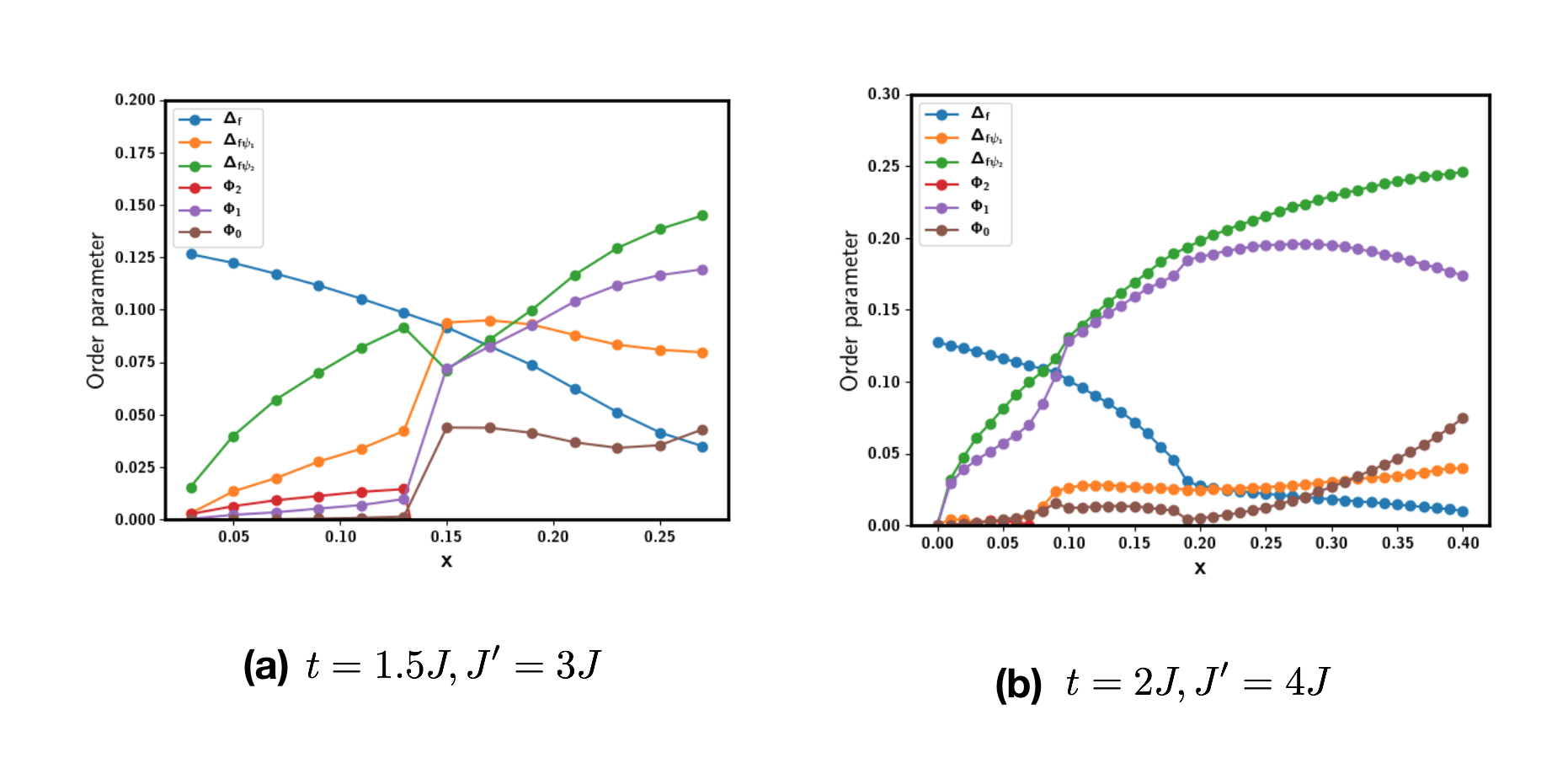
In the following we try to determine the order parameters in the level of mean field theory. From solving the self consistent equations (shown in Append.  C), we get a plot of order parameters shown in Fig. 1. The dominant order parameters are $\Phi_{1}$, $\Delta_{f\psi_{2}}$ and $\Delta_{f}$. First let us ignore $\Delta_{f}$. We want to show that $\Phi_{1}$ and $\Delta_{f\psi_{2}}$ are Kondo couplings which merge $f,\psi_{1},\psi_{2}$ to form a conventional Fermi liquid. We have two $U(1)$ gauge field: $a$ is shared by $f$ and $\psi_{a}$, $\alpha$ parameterizes part of the $SU(2)$ gauge field generated by $\tau_{z}$. $f$ couples to $a$, $\psi_{1}$ couples to $\frac{1}{2}a+\frac{1}{2}\alpha+\frac{1}{2}A$. Now, $\psi_{2}$ couples to $\frac{1}{2}a-\frac{1}{2}\alpha+\frac{1}{2}A$. The condensation of $\Phi_{1}$ and $\Delta_{f\psi_{2}}$ locks the gauge fields to be $a=-A$ and $\alpha=-2A$. Then $f$ and $\psi_{1}$ couple to $-A$ while $\psi_{2}$ couples to $A$. This means that we can view $\psi_{2}$ as physical hole operator, while viewing $f,\psi_{1}$ as physical electron operator. Let us redefine $\tilde{f}_{i;\sigma}=f^{\dagger}_{i;\sigma}$ and $\tilde{\psi}_{i;1\sigma}=\psi^{\dagger}_{i;1\sigma}$. Then $\tilde{f},\tilde{\psi}_{1},\psi_{2}$ are all hole operators and they hybridize together to form a Fermi liquid with large Fermi surfaces, as shown in Fig. 2.

At small $x$, we find $\Delta_{f}\neq 0$, thus the ground state is a d-wave superconductor. $\Delta_{f}$ decreases with doping, resulting a dome similar to that of the cuprates. Here in the under-doped region, $T_{c}$ is decided by the on-set of $\Phi_{1}$ and $\Delta_{f\psi_{2}}$. In certain sense, the destruction of the superconductor is from "Kondo breaking down".

In the above we used $J^{\prime}=4J$ to get stable Fermi liquid/superconductor. For smaller $J^{\prime}/J$, there is zero or just one Kondo coupling when $x<x_{c}$ in the mean field calculation, resulting in a "pseudogap metals" phase or a FL* phase in under-doped region. It is not clear whether this is just an artifact of mean field treatment. Our mean field theory suggests that the phase diagram at small $x$ region is like that shown in Fig. 3. One can see that this phase diagram is similar to that from slave boson theory for cupratesLee et al. 2006. The difference is that here the $T_{c}$ (or coherence scale) is determined by "Kondo breaking down" instead of slave boson condensation.

Role of Nd orbital In the undoped sample, resistivity shows metallic behavior above $50$ K and an upturn below $50$ K. The metallic behavior can be attributed to electron pocket from Nd orbitalBotana and Norman 2019; Hepting et al. 2019; Sakakibara et al. 2019; Wu et al. 2019, leading to ‘self doping’. We can extend our $t-J$ model to include the Nd orbital (see Appendix.  F):

where $d^{\dagger}_{i}$ creates a hole for Nd orbital. Note here $c_{i}^{\dagger}$ creates the spin-one doublon and thus is different from the model in Ref. Hepting et al. 2019. If the density of Nd holes is $n_{Nd}=1-\delta$, then the density for spin-one holes is $n_{c}=x+\delta$. In principle $\delta$ can have both doping and temperature dependence. Especially, $\delta$ is expected to decrease when we increase $x$Botana and Norman 2019. One can see that $n_{c}=\delta\neq 0$ even for $x=0$ if there is electron pocket from Nd in the Fermi level. This "self-doping" effect can explain why the undoped compound is metallic and does not have magnetic order.

Conclusion In summary, we propose a novel $t-J$ model with spin one hole (doublon in hole picture) to model the hole doped NdNiO₂. We introduce two distinct parton theories to analyze this unconventional model. Especially, we find that a Fermi liquid or d wave superconductor is possible in this model, arising from the "Kondo resonance" between the spin one doublon and spin $1/2$ singly occupied state. This suggests that a combination of "heavy fermion physics" and "cuprate physics" may emerge in this new model. We hope the proposed model and the parton framework introduced in this paper will motivate further theoretical and numerical studies, as well as experiments probing the spin-orbital nature of doped holes in this new superconductor.

Acknowledgement YH.Z thanks T. Senthil and Dan Mao for previous collaborations and discussions on $SU(4)$ Hubbard model and spin-one spin liquid, which inspired the proposal of the parton constructions in this paper. A. V. thanks Z. X. Shen and Julia Mundy for discussions. This work was supported by a Simons Investigator Grant (A.V.).

References

- Li et al. (2019) D. Li, K. Lee, B. Y. Wang, M. Osada, S. Crossley, H. R. Lee, Y. Cui, Y. Hikita, and H. Y. Hwang, Nature 572, 624 (2019).
- Anisimov et al. (1999) V. I. Anisimov, D. Bukhvalov, and T. M. Rice, Phys. Rev. B 59, 7901 (1999).
- Chaloupka and Khaliullin (2008) J. c. v. Chaloupka and G. Khaliullin, Phys. Rev. Lett. 100, 016404 (2008).
- Lee and Pickett (2004) K.-W. Lee and W. E. Pickett, Phys. Rev. B 70, 165109 (2004).
- Botana and Norman (2019) A. S. Botana and M. R. Norman, arXiv e-prints , arXiv:1908.10946 (2019), arXiv:1908.10946 [cond-mat.supr-con] .
- Sakakibara et al. (2019) H. Sakakibara, H. Usui, K. Suzuki, T. Kotani, H. Aoki, and K. Kuroki, arXiv e-prints , arXiv:1909.00060 (2019), arXiv:1909.00060 [cond-mat.supr-con] .
- Hepting et al. (2019) M. Hepting, D. Li, C. J. Jia, H. Lu, E. Paris, Y. Tseng, X. Feng, M. Osada, E. Been, Y. Hikita, Y. D. Chuang, Z. Hussain, K. J. Zhou, A. Nag, M. Garcia-Fernandez, M. Rossi, H. Y. Huang, D. J. Huang, Z. X. Shen, T. Schmitt, H. Y. Hwang, B. Moritz, J. Zaanen, T. P. Devereaux, and W. S. Lee, arXiv e-prints , arXiv:1909.02678 (2019), arXiv:1909.02678 [cond-mat.supr-con] .
- Nomura et al. (2019) Y. Nomura, M. Hirayama, T. Tadano, Y. Yoshimoto, K. Nakamura, and R. Arita, arXiv e-prints , arXiv:1909.03942 (2019), arXiv:1909.03942 [cond-mat.supr-con] .
- Gao et al. (2019) J. Gao, Z. Wang, C. Fang, and H. Weng, arXiv preprint arXiv:1909.04657 (2019).
- Ryee et al. (2019) S. Ryee, H. Yoon, T. J. Kim, M. Y. Jeong, and M. J. Han, arXiv preprint arXiv:1909.05824 (2019).
- Zhang et al. (2019a) H. Zhang, L. Jin, S. Wang, B. Xi, X. Shi, F. Ye, and J.-W. Mei, arXiv preprint arXiv:1909.07427 (2019a).
- Zhang and Rice (1988) F. Zhang and T. Rice, Physical Review B 37, 3759 (1988).
- Zaanen et al. (1985) J. Zaanen, G. Sawatzky, and J. Allen, Physical Review Letters 55, 418 (1985).
- Jiang et al. (2019) M. Jiang, M. Berciu, and G. A. Sawatzky, arXiv e-prints , arXiv:1909.02557 (2019), arXiv:1909.02557 [cond-mat.supr-con] .
- Kojima et al. (1995) K. Kojima, A. Keren, L. Le, G. Luke, W. Wu, Y. Uemura, K. Kiyono, S. Miyasaka, H. Takagi, and S. Uchida, Journal of magnetism and magnetic materials 140, 1657 (1995).
- Zhang et al. (2017) J. Zhang, A. Botana, J. Freeland, D. Phelan, H. Zheng, V. Pardo, M. Norman, and J. Mitchell, Nature Physics 13, 864 (2017).
- Wu et al. (2019) X. Wu, D. Di Sante, T. Schwemmer, W. Hanke, H. Y. Hwang, S. Raghu, and R. Thomale, arXiv e-prints , arXiv:1909.03015 (2019), arXiv:1909.03015 [cond-mat.supr-con] .
- Hirsch and Marsiglio (2019) J. Hirsch and F. Marsiglio, Physica C: Superconductivity and its Applications , 1353534 (2019).
- Singh (2019) N. Singh, arXiv preprint arXiv:1909.07688 (2019).
- Zhang et al. (2019b) G.-M. Zhang, Y.-F. Yang, and F.-C. Zhang, arXiv preprint arXiv:1909.11845 (2019b).
- (21) For square planar symmetry, it may also be possible that orbital has lower energy than orbital in hole picture. In this case the hopping in direction should be negligible.
- Zener (1951) C. Zener, Physical Review 82, 403 (1951).
- Anderson (1987) P. W. Anderson, science 235, 1196 (1987).
- Lee et al. (2006) P. A. Lee, N. Nagaosa, and X.-G. Wen, Reviews of modern physics 78, 17 (2006).
- Zhang and Mao (2019) Y.-H. Zhang and D. Mao, arXiv preprint arXiv:1906.10132 (2019).
- Senthil et al. (2004) T. Senthil, M. Vojta, and S. Sachdev, Physical Review B 69, 035111 (2004).
- Frésard and Kotliar (1997) R. Frésard and G. Kotliar, Physical Review B 56, 12909 (1997).
- Brinckmann and Lee (2001) J. Brinckmann and P. A. Lee, Physical Review B 65, 014502 (2001).
- Nandkishore et al. (2012) R. Nandkishore, M. A. Metlitski, and T. Senthil, Physical Review B 86, 045128 (2012).
Appendix A Microscopic derivation of model with spin one doublon
A.1 Distinction from cuprates: spin one hole
Because the oxygen orbital is far away from Fermi level in , the doped hole will enter the orbitals. From the LDA+U calculation Botana and Norman 2019; Hepting et al. 2019, the energy splitting of the two orbitals is eV and smaller than the interaction scale. Therefore we need to include both and orbitals. We choose to study the following model in hole picture: