Transition from Inspiral to Plunge:
A Complete Near-Extremal Trajectory and Associated WaveformPreprint: APS/123-QED
Abstract
We extend the Ori and Thorne (OT) procedure to compute the transition from an adiabatic inspiral into a geodesic plunge for any spin, with emphasis on near-extremal ones. Our analysis revisits the validity of the approximations made in OT. In particular, we discuss possible effects coming from eccentricity and non-geodesic past-history of the orbital evolution. We find three different scaling regimes according to whether the mass ratio is much smaller, of the same order or much larger than the near extremal parameter describing how fast the primary black hole rotates. Eccentricity and non-geodesic past-history corrections are always sub-leading, indicating that the quasi-circular approximation applies throughout the transition regime. However, we show that the OT assumption that the energy and angular momentum evolve linearly with proper time must be modified in the near-extremal regime. Using our transition equations, we describe an algorithm to compute the full worldline in proper time for an extreme mass ratio inspiral (EMRI) and the resultant gravitational waveform in the high spin limit.
pacs
Valid PACS appear hereI Introduction
The LIGO observation of the transient gravitational wave (GW) signal from the collision of two stellar mass black holes PhysRevLett.116.061102 in September 2015 spectacularly opened the new field of gravitational wave astronomy. By the end of the O2 observing run in August 2017, the LIGO/Virgo detectors had observed ten binary black hole mergers and a single binary neutron star inspiral scientific1811gwtc. This handful of observations has already had a profound impact on our understanding of the astrophysics of compact objects and ruled out a number of modified theories of gravity baker2017strong; langlois2018scalar; ezquiaga2017dark; sakstein2017implications; boran2018gw170817. During the ongoing O3 observing run new events are being reported at the rate of one per week, so these constraints are rapidly improving. However, the masses of the objects being observed are all in the range of –, which is determined by the frequency sensitivity of the instruments sathyaprakash2009physics. Black holes with much higher masses are expected to exist in the centres of most galaxies croton2006many and will be even stronger sources of GWs, but these waves will be at millihertz frequencies which are inaccessible to ground-based detectors due to the seismic noise background.
The launch of the Laser Interferometer Space Antennae (LISA) 2017arXiv170200786A, scheduled for 2034, will open the millihertz band from –Hz for the first time. Expected sources in this frequency band include massive black hole binaries, cosmic strings and extreme mass ratio inspirals (EMRIs). Detection of these sources, and estimation of their parameters, will rely on the comparison of accurate theoretical models of the expected gravitational waveforms to the observed data. Building these models for LISA is extremely challenging, in particular for EMRIs, which are expected to have a very rich structure and to be observed for hundreds of thousands of waveform cycles prior to merger with the central object amaro2007intermediate. In this paper we focus on modelling of a particular class of EMRIs, in which the central black hole has very large angular momentum (spin). All of the LIGO observations to date are consistent with zero or small spin scientific1811gwtc, but the massive black holes that will be probed by LISA are a different population. These black holes are observed in high accretion states as quasars, and accretion tends to spin the black holes up. Semi-analytic models predict that the typical spins of these objects are 2014ApJ…794..104S.
The maximum spin of massive black holes is a quantity of fundamental interest for understanding the origin of black holes in the Universe. It was shown by Thorne 1974ApJ…191..507T that the angular momentum of black holes being spun up through thin disc accretion saturates at a limit of where an equilibrium is reached between spin up by accreted material and spin down by captured retrograde photons. Black holes with higher spin could in principle be formed directly in the early Universe and for sufficiently high mass these black holes can retain spins above the Thorne limit for a Hubble time arbey2019any. A direct observation of a system with spin above the Thorne limit would thus have profound implications for our understanding of the origin and growth of black holes. It is therefore important to understand how well observations of EMRIs can constrain the spin of near-extremal black holes and to determine this we first need to build accurate representations of the gravitational waves emitted by such systems.
The near extremal limit is also relevant for more theoretical considerations. Indeed, as the primary rotates faster, its Hawking’s temperature decreases because the distance between the inner and outer horizons in Boyer-Lindquist (BL) coordinates reduces according to
| (1) |
where and the dimensionless Kerr spin parameter. The existence of a double pole in the function determining the black hole horizons in this limit is responsible for an enhancement of symmetry in the near horizon geometry of the Kerr black hole Bardeen:1999px, a feature that remains true for any extremal black hole Kunduri:2007vf. This enhancement of symmetry from time translations to the conformal group has allowed several groups to analytically solve the master Teukolsky equation in the presence of the in spiraling probe particle leading to an analytic expression for the energy fluxes carried by the gravitational waves generated by this source Porfyriadis:2014fja; Hadar:2014dpa; Hadar:2015xpa; 2015PhRvD..92f4029G; 2015PhRvD..92f4029G; van2015near; Hadar:2016vmk; 2016CQGra..33o5002G; 2016CQGra..33o5002G; 2018arXiv180403704C; compere2018_NHEK. This provides a very exciting opportunity where analytic tools developed in the high energy theoretical physics community can provide accurate predictions to generate gravitational waveform templates. Future observations using such templates will be directly testing these theoretical predictions.
It has already been shown that gravitational waveforms emitted by these sources contain unique qualitative features that provide a smoking gun for the existence of near-extremal systems 2016CQGra..33o5002G. The amplitude of an EMRI waveform (averaged over a suitable amount of orbits) typically increases linearly in time for moderate spin . It was shown in 2016CQGra..33o5002G that the amplitudes of these signals dampen in the high spin limit due to behaviour of the flux close to the horizon. There has been progress in modelling the inspiral from radial infinity to the innermost stable circular orbit (ISCO) 2016CQGra..33o5002G, by integrating the geodesic equations in the near horizon geometry of the Kerr black hole kapec2019particle and exploiting the enhanced set of symmetries to compute the energy fluxes for more source trajectories compere2018_NHEK. However, no one has focused on providing a model which encapsulates the inspiral and plunge in the limit of high spins. This is precisely what this paper seeks to do.
In this work, we build such a model for an EMRI comprised of a small compact object of mass gravitationally bound to a supermassive Kerr black hole of mass and study the transition from an adiabatic inspiral into a geodesic plunge for any spin of the primary black hole. This transition to plunge was originally discussed by Ori and Thorne (OT) 2000PhRvD..62l4022O for moderate values of the spin in the limit of small mass ratios. A similar but independent analysis conducted by Buonanno and Damour in buonanno2000transition solved the problem for Schwarzschild black holes with arbitrary (reduced) mass ratio. The technical reason why high spins require a separate discussion is because of the existence of a second independent small parameter competing with the mass ratio . This new parameter is the near-extremal parameter encoding the distance of the spin parameter from its upper/lower bound, since Kerr black holes have spin parameters . Since the dynamical equations describing the transition depend on the spin, the near extremal limit, i.e. , modifies the original scaling discussed by OT. The transition to plunge for near-extremal EMRIs was previously considered in kesden2011transition and our work clarifies and extends those results in a number of ways. We point out the physical interpretation of the mathematical procedure used in that paper, identify a missing term in the near-extremal regime and incorporate recent analytic results for the near-extremal energy flux for the first time.
In this paper, we will first review the treatment of the transition regime given by OT in 2000PhRvD..62l4022O. We analyse their methodology and approximations and carefully estimate the scaling of terms that are being omitted. In each of 2000PhRvD..62l4022O; sundararajan2008transition; Transition_Inspiral_Scott_Hughes the notion of eccentricities and non-circular motion was ignored. We discuss the potential growth of eccentricities before and during the transition regime and find that corrections to our equations due to eccentric motion are sub-leading for any spin. We identify three separate transition regimes, each with a slightly different equation of motion: , and . We then discuss a numerical algorithm to generate full inspiral trajectories in Boyer-Lindquist coordinates, alongside the corresponding evolution of the integrals of motion and . Finally, we extend the waveform from the inspiral only results of 2016CQGra..33o5002G to include the plunge in the regime .
This paper is organised as follows. In section II, we review the properties of equatorial and circular orbits in the Kerr black hole and, in section II.1, we review and compare the results describing gravitational fluxes emitted by circular EMRIs as a function of the spin. In section III we set-up the master transition equation of motion in general and, in subsection III.3, we estimate corrections due to eccentricity and non-geodesic past-history of the orbital evolution. The transition equations of motion in the three different sxcaling regimes are described in subsections III.4, III.5 and III.6 respectively. The numerical scheme to integrate our transition equations of motion for the regime is presented in section IV.1. We describe how to generate a near-extremal EMRI gravitational waveform encapsulating inspiral and plunge in subsections IV.2 and IV.3. We finish with a summary of our main results in section V.
Notation: Any quantity carrying a tilde refers to a dimensionless quantity in units of the primary mass M, i.e. , , , and , but we keep as the dimensionless Kerr spin parameter with no tilde. Dotted quantities (eg ) denote coordinate time derivatives of that quantity. Finally, expressions or, for brevity, stress that both and scale in the same way with the small parameters under consideration. We impose geometrized units by setting the constants .
Note added. In the final stages of this work, we became aware of overlapping results that were independently obtained in Geoffrey_Transition.
II Preliminaries
In Boyer-Lindquist (BL) coordinates , the motion of a point particle with mass in a Kerr black hole on the equatorial plane () is given by Schmidt:2002qk
| (2) | ||||
| (3) | ||||
| (4) |
where the largest root of corresponds to the outer horizon
denotes proper time in units of the Kerr black hole mass and is the dimensionless spin parameter .
The particle is on a prograde (retrograde) orbit if it follows the same (opposite) direction as the rotation of the primary hole. Prograde (retrograde) orbits correspond to while keeping the azimuthal component of the angular momentum . Since retrograde orbits do not reach the near horizon geometry of the primary black hole in the near-extremal limit (see appendix B), while prograde orbits do, we only consider the latter from here on.
For an equatorial orbit to be circular, the BL radial coordinate must be constant and to be stable, the latter must be at a minimum of the potential in (2) so that
These conditions determine the energy and angular momentum of these orbits to be Chandrasekhar:579245
| (5) | ||||
| (6) |
Substituting (5)-(6) into (3)-(4) gives rise to
| (7) | |||||
| (8) |
whose ratio defines the angular velocity of the particle
| (9) |
Equatorial circular orbits are also known to satisfy the identity 1998PhRvD..58f4012K
| (10) |
where we stress the equality holds for any circular orbit labelled by . Differentiating (10) with respect to , we can derive further equalities satisfied for any such orbits. The ones below
| (11) | |||||
| (12) | |||||
will play a role in our analysis later on.
The innermost stable circular orbit (ISCO) is the marginal circular stable orbit satisfying
| (13) |
The last equality, describing marginality, allows to solve for its radius as a function of the spin bardeen1972rotating
| (14) | ||||
This is the last radii before plunging into the horizon occurs. In appendix A, we derive general formulas for (13) and higher order derivatives of , which are valid for any spin , when evaluated at ISCO that will be relevant in the rest of this work.
For near-extremal Kerr black holes, it is natural to introduce the near extremal parameter
| (15) |
to mathematically capture the large spin limit . For these black holes, the ISCO location can be expanded in
| (16) |
and the physical parameters of this marginal orbit reduce to
| (17) | ||||
| (18) | ||||
| (19) |
Notice for prograde orbits, whereas it is for retrograde ones, as mentioned below (133). This further justifies our interest in prograde orbits in the near extremal limit.
II.1 Gravitational Wave Flux
For equatorial orbits, the motion of a (point) particle on the Kerr spacetime background generates gravitational waves carrying energy and angular momentum, either escaping towards infinity or being absorbed by the horizon of the primary hole.
Due to energy and angular momentum conservation, the orbit averaged rates of change and satisfy and , where the averaged gravitational wave dissipative fluxes are
| (20) | ||||
determined in terms of the time-averaged and components of the dissipative self-force normalised by the component of the four velocity . These quantities are discussed in more depth in the next subsection III.1 (see appendix C, in particular the discussion around (155), for a derivation of relations such as (20)). Notice we split these fluxes into their horizon and asymptotic infinity contributions in the right hand side. We stress here this flux balance law only holds for adiabatically evolving binaries forcing the small mass ratio limit . The (orbit-averaged and dissipative) gravitational wave fluxes are determined by solving the Teukolsky equation in the presence of the point particle source teuk73; sasaki82; hu1; 2002PhRvD..66d4002G; dras. From hereon, to avoid cumbersome notation, we shall drop the angled-brackets to denote time-averaging and simply write, for example, .
In 2000PhRvD..62l4021F, Finn and Thorne (F&T) parameterise the energy flux as the (Peters and Mathews peters1963gravitational) leading order post newtonian correction with an extra general relativistic correction factor
| (21) |
These fluxes are spin dependent and are typically computed through numerical means. See the tables in 2000PhRvD..62l4021F for some of the values of these relativistic corrections.
As we increase the spin of the black hole, the two roots of the function determining the outer and inner horizons of the rotating black hole coincide in the extremal limit . In this limit, the geometry close to the horizon of the black hole, which can be isolated using the change of coordinates
| (22) |
with , has an enhancement of symmetry from , i.e. time translations and rotational symmetry, to . The resulting near horizon geometry is warped AdS2 over a 2-sphere. The enhanced , the isometry group of AdS2, includes the scaling symmetry and . This was already observed in the original work Bardeen:1999px and it is true for any extremal black hole Kunduri:2007vf.
Larger symmetry in physics implies larger kinematic constraints which can provide further analytic control over the given problem, in this case, the calculation of the gravitational wave fluxes (20). It is precisely the emergence of this conformal group and the use of asymptotic expansion matching methods that allowed to find analytic expressions for these energy and angular momentum fluxes for equatorial circular orbits close to the horizon Porfyriadis:2014fja; Hadar:2014dpa; Hadar:2015xpa; 2015PhRvD..92f4029G; Hadar:2016vmk; 2016CQGra..33o5002G; compere2018_NHEK. This body of work led to the simple relationship for the flux given in 2016CQGra..33o5002G
| (23) |
The quantities and are constants representing how much wave emission goes towards the horizon and infinity respectively. These constants are given analytically in equations (76) and (77) of 2015PhRvD..92f4029G. Numerically evaluating them and summing the contribution of the first modes gives and .
The flux (23) is only reliable when working with near extremal black holes and interested in near horizon physics. This fact can be checked by comparing the exact fluxes (21), using exact results found in the black hole perturbation toolkit (BHPT), with the near extremal approximation (23). This comparison is shown in figure 1. Fixing the radial coordinate to and varying the spin parameter , we observe in Table (1) that as , the NHEK flux (23) converges towards the exact value computed using the BHPT. Furthermore, fixing the spin parameter to , as in figure (1), the NHEK flux (23) provides a nearly-perfect agreement up to a coordinate radii . The reason for the (extremely small) discrepancy at the ISCO is because Eq.(23) is only valid for and we consider .


| 0.0264197 | 0.0261523 | 0.0002674 | |
| 0.0129344 | 0.0125200 | 0.0004143 | |
| 0.0061516 | 0.0059484 | 0.0002031 | |
| 0.0028875 | 0.0028082 | 0.0000793 | |
| 0.0013472 | 0.0013193 | 0.0000280 | |
| 0.0006273 | 0.0006176 | 0.0000097 | |
| 0.0002915 | 0.0002883 | 0.0000031 | |
| 0.0001354 | 0.0001344 | 0.0000009 |
III The Transition Equation of Motion
In this section we revisit the earlier work by OT 2000PhRvD..62l4022O describing how a small body following an initial equatorial circular orbit around the large black hole inspirals and eventually transitions into a plunging trajectory falling into the black hole.
Our discussion is organised as follows. First, we analyse in section III.1 the effects arising from the radial self-force in the vicinity of the ISCO on the dynamics of this small body, justifying the starting point in OT. Second, assuming the dissipative fluxes of energy and angular momentum for quasi-circular and equatorial orbits are still related as in circular orbits apostolatos1993gravitational; 1998PhRvD..58f4012K
| (24) |
we derive in section III.2 the transition equation for arbitrary black hole spins without the OT assumption that both energy and angular momenta evolve linearly in proper time . Third, given the quasi-circular nature of our assumed orbits, we argue in section III.3 there can be corrections to (24) of the form
| (25) |
whose scaling behaviour on the trajectory of the small body is determined. Finally, in sections III.4-III.6, we discuss in great detail the existence of three different scaling regimes in our transition equation, depending on the black hole spin, paying special attention to the near-extremal ones which contain new physics. We show the corrections due to (25) are subleading in all the regimes.
III.1 The self-force
This subsection shows both that quasi-circular and equatorial orbits have vanishing dissipative effects and the conservative piece of the radial self-force can be neglected close to the ISCO.
Consider the radial geodesic equation, Eq. (2). Differentiating it with respect to proper time, one obtains
| (26) |
It is shown in Appendix C this is equivalent to
| (27) |
Hence, the terms on the left hand side of eq. (26) correspond to the usual ones for geodesic motion, whereas the one on the right hand side can be understood as the perturbing force exerted on the particle driving energy and angular momentum loss due to gravitational wave emission.
In Mino:2003yg, Mino recognised that the forcing term for general geodesic motion can perturbatively be split into a radiative reactive dissipative and a conservative piece at first order in the mass ratio
| (28) |
More details on this splitting can be found in barack2018self.
For circular orbits, as considered by OT, the dissipative fluxes of energy and angular momentum are related by apostolatos1993gravitational; 1998PhRvD..58f4012K
| (29) |
Hence, the dissipative part of the self-force vanishes, leading to
| (30) |
which is precisely Eq.(3.10) of OT in 2000PhRvD..62l4022O. A gauge invariant way to quantify the leading order in effect on the trajectory due to is to study the orbital velocity (see barack2018self for a review). This generates a shifted orbital velocity with respect to the Kerr orbital velocity at ISCO given by barack2009gravitational; van2017self
| (31) |
with the quantity discussed in depth and independently (numerically) calculated in both isoyama2014gravitational; van2017self. According to van2017self, . Hence, for all spins, and since , it follows that for
| (32) |
It is further shown in van2017self that as in an averaged sense11 1 is shown to actually oscillate around this limiting value as . This phenomenon is non-trivial and still not well understood today. See van2017self for more details.. Using Eq.(19) in the high spin limit and , equation (31) becomes
| (33) |
This implies that the change in the orbital velocity at the ISCO due to conservative self-force effects is an quantity.
Since is related to the shifted Boyer-Lindquist radial coordinate at the ISCO by
| (34) |
it follows, using eq.(33), that the “radial thickness”
| (35) |
differs by an quantity when including the conservative self-force effects.
It will be shown in this paper that there are three different transition regimes depending on the ratio of and . The “radial thickness” of the transition in each regime scales according to
- •
For ,
- •
For ,
- •
For .
Thus, the effect of the conservative piece of the self-force is subleading in all regimes. For this reason, like in the original OT analysis, we shall ignore these effects.
III.2 Transition Equation - Generalities
To discuss the evolution of the orbit, we pursue the following strategy : we assume the corrections in (25) are subleading, and once the scaling behaviour of the different dynamical regimes is identified, we double check the consistency of our original assumption.
To evolve the orbit, OT used the circular flux relationship (29) and additionally assumed that the energy and angular momentum evolve linearly in proper time throughout the transition regime
| (36) | ||||
In our analysis of the transition, we will not assume a strict equality in Eq.(36). Instead, we will keep track of the evolution of , as also considered in kesden2011transition.
OT proposed to analyse the transition to the plunging geodesic by expanding (26) around the ISCO trajectory , since the latter provides the natural starting point for the plunging trajectory for equatorial and circular orbits. It is physically natural to introduce the new variables , and
| (37) | ||||
to study the inspiral evolution of the small body perturbatively around the primary. The presence of is for technical convenience.
Instead of expanding (26), we find it more convenient to expand (2). Our conclusions do not depend on this choice. The latter is given by
| (38) |
Since is quadratic in and , we have ignored the derivatives
| (39) |
Plugging the perturbative variables (37), using the definition of the coefficients (120) and the results in (121)-(123), one can rewrite the general transition equation as
| (40) |
where is defined by
| (41) | ||||
Notice that at leading order in . Hence, it encodes the deviations from the OT approximation (36).
The time evolution of near is controlled by the fluxes and the angular velocity. Throughout a quasi-circular inspiral far from ISCO, the compact object inspirals on a sequence of circular geodesics defined by the constants of motion and , as given in Eq (5) and Eq.(6) respectively. The evolution of the constants of motion is linked through Eq. (29) above, which simply states that circular geodesics evolve into circular geodesics. It can be shown that solutions to the Teukolsky equation for circular orbits obey this condition CircularOrbitsOri; 1998PhRvD..58f4012K. For circular evolutions we therefore see that
| (42) | ||||
where we expanded to first order in and approximated for constant defined by
| (43) |
Thus we deduce that for circular inspirals close to . We shall see that these corrections are indeed subleading in the regime considered by OT 2000PhRvD..62l4022O. However, they will not be negligible for near-extremal black holes.
III.3 Corrections arising from deviations from adiabatic nearly-circular inspiral
Given our assumption that the orbit is nearly circular when it reaches the transition regime, one expects corrections to the relation (29) between the fluxes of energy and angular momentum satisfied for an exactly equatorial circular adiabatic inspiral. We discuss below two possible physical effects giving rise to such corrections : eccentricity and the non-geodesic past-history of the orbital evolution. These will give rise to the corrections (25).
Eccentricity can lead to corrections to the transition equation which we will discuss further below, but eccentricity corrections to the fluxes tend to be suppressed during the transition regime. This is because the transition, for an arbitrary eccentric inspiral, corresponds to the orbit passing over the maximum of the effective potential given by Eq.(2). The radial velocity throughout the transition regime is therefore always small, while the angular velocity remains . Hence the orbit looks very much like a circular orbit, even if it is technically eccentric or even plunging. For nearly-circular transitions, the orbit is passing over a point of inflection of the effective potential and corrections to this approximately-circular assumption are even smaller.
Corrections from non-geodesic past-history enter because the self-force acting on the small object at a particular time is generated by the intersection of the particle world line with gravitational perturbations generated by the orbital motion in the immediate past LRP. The self-force acting on the orbit when it is at a particular radius will therefore have corrections that depend on how far, in radius, the orbit has moved over the relevant past-history. The latter is determined by the dominant, azimuthal, timescale, and is an quantity, when expressed in coordinate time 22 2 If we are more conservative, we could assume that the timescale for radial oscillations is the appropriate averaging timescale. This is not , but , the scaling of the time coordinate in the transition zone. While this condition is more restrictive we will see below that even this condition does not change the conclusion that past-history corrections can be ignored in the transition zone.. The orbital radius therefore changes by an amount of over the relevant past-history. This is the scaling of the fractional change in the fluxes, and since , the non-geodesic past-history corrections to the coordinate-time fluxes thus scale like . In the regime , considered by OT, and discussed in Section III.4, can be considered and so the scaling of this correction is . This is the first type of correction in Eq.(25). In the adiabatic inspiral phase, these corrections are and form part of the second-order component of the self-force. However, in the transition phase these corrections can be larger.
We have argued above that eccentricity corrections to the fluxes should be suppressed in the transition regime. We now make this more concrete. Eccentricity corrections to the fluxes enter as fractional corrections of , since corrections to the orbit at linear order in eccentricity are oscillatory and average to zero over a complete orbit 1998PhRvD..58f4012K. The corrections to the coordinate time fluxes thus scale like (which is in the OT regime discussed in Section III.4). This is the second type of correction in Eq.(25). If these corrections are to be small relative to the non-geodesic past-history corrections, we need . In the transition zone we will see that the proper time scales like , where is the distance from the ISCO, regardless of the spin of the primary. For non near-extremal black holes, i.e., those with , proper time and coordinate time scale in the same way and the scaling of is therefore the same as that of . The constraint we obtain on eccentricity is therefore . However, there is also a geometric constraint, which is that the variation in the orbital radius due to eccentricity should be small compared to the variation due to radiation reaction through the transition zone. The latter is the scaling of , while the former is a quantity of , so we deduce an additional constraint , the latter inequality following from the fact that is a small quantity throughout the transition. We deduce that the geometrical constraint is stronger than the flux-correction constraint in the regime . In the near-extremal regime, , and so the constraint on the eccentricity changes to if these corrections are to be subleading. This is then more stringent than the geometric constraint. However, in this regime we will see below that eccentricity cannot grow until deep inside the transition zone, so even the more stringent constraint is easily satisfied.
Eccentricity during the transition can arise either from the presence of residual eccentricity prior to the start of the transition zone, or due to the excitation of eccentricity during the transition. The latter manifests itself as additional terms in the transition equation, the existence of which we will check for carefully in our analysis. To understand the former, we need to analyse the growth of eccentricity during the adiabatic inspiral. We will assume that at the beginning of the inspiral the orbit is nearly circular. It was shown in 1998PhRvD..58f4012K that, for small eccentricity, the evolution of eccentricity under radiation reaction takes the form , where is the mean orbital radius and is an eccentricity defined such that the orbital apoapsis is at . For large , and so the eccentricity decreases. In this regime any small eccentricity that is excited by small perturbations arising due to inspiral evolution or other effects is damped away and does not grow. However, for all spins , as the innermost stable circular orbit (or separatrix) is approached the sign of changes and is greater than zero in the vicinity of the ISCO. This means that orbits near to the separatrix are unstable to eccentricity growth. We would therefore expect any eccentricity that is excited to begin to grow.
Denoting , Kennefick 1998PhRvD..58f4012K showed that the evolution of the orbital parameters, for small eccentricity, was governed by equations of the form
| (44) | ||||
| (45) | ||||
| where | ||||
Both and are components of the self-force, which can be evaluated by solving the Teukolsky equation. The quantity is in fact a linear combination of quantities that are time derivatives and so the above equation takes the same form for any choice of time coordinate with respect to which to evaluate the fluxes. Kennefick’s analysis used coordinate time and so we make the same choice in the following discussion. An explicit expression for is given in 1998PhRvD..58f4012K and the quantity is the energy flux given in (20). Numerical calculations show that these are finite quantities of throughout parameter space. The first term in the eccentricity evolution equation vanishes for evolution driven by gravitational radiation reaction, while the quantity is singular at the ISCO. Therefore, close to ISCO the eccentricity evolution takes the form
| (46) |
Notice that the expression is entirely geodesic and independent of the energy flux . For non-extremal spin, both and have simple poles at and there is a simple zero in the term in the numerator. Therefore as ISCO is approached the eccentricity evolves as
| (47) |
with as before, and denotes the eccentricity when and . The exponent is given by
| (48) |
and . We find that for all . The behaviour for near-extremal black holes is slightly different, which we will discuss further below.
For extremal black holes the various factors in the expression for have repeated roots at the ISCO. To understand the behaviour for near-extremal black holes we therefore need to do an expansion in both and . This takes the form
| (49) |
The terms omitted from both the numerator and denominator above are in . The ratio , agreeing with the result for found above. However, for , the behaviour is not dominated by this term, but by the terms from in the numerator and from in the denominator. The leading order behaviour in this regime is therefore
| (50) |
This is also exponential, but we find the ratio , i.e., it is greater than zero and therefore the eccentricity decreases exponentially until we reach the regime . This is the statement that the critical curve, where the sign of the eccentricity evolution changes, is in the near-horizon region, which is consistent with results in 2002PhRvD..66d4002G. We conclude that for near-extremal black holes, eccentricity can only grow once the inspiraling object is already very close to the ISCO, which is typically already inside the transition zone.
To complete this discussion we need to determine the scaling of the initial eccentricity . If the orbit is truly circular then the eccentricity remains zero, so there must be some mechanism to excite an initial eccentricity which can then grow. Eccentricity can be excited by other physical processes, such as the presence of perturbing material, e.g., dust, or gravitational interactions with third bodies. Those processes are important, but in the pure-vacuum case eccentricity could still in principle be excited by the evolution under radiation reaction. We argued earlier that corrections to the fluxes far from the horizon scale like which is during the adiabatic inspiral. These corrections mean that the first term in Eq. (45) is no longer exactly zero. Setting that term to we find an evolution equation of the form . After a few orbits the eccentricity is then . This eccentricity induced by second order corrections to the evolution is damped by the process described above, until we reach the critical curve where it grows, eventually exponentially near the ISCO. This suggests appropriate initial conditions are and .33 3 A natural continuation of this argument would be to say that the second-order self-force induced corrections continue to drive eccentricity growth, over the whole of the inspiral, lasting a coordinate time , leading to a final eccentricity of , which can be larger than the eccentricity grown through the mechanism discussed here. However, this assumes that the eccentricity grows coherently and monotonically. In practice, once the eccentricity is , the radial motion due to eccentricity becomes larger than the amount the radius evolves over the relevant past-history that determines the self-force and so the argument that the latter is the dominant contribution to corrections no longer applies. Knowledge of the second-order self-force would be required to fully explore the further evolution of the eccentricity and this is not currently available. However, we expect that the growth of initial eccentricities of through the instability mechanism will be the dominant contributor to the residual eccentricity in the transition zone. We note that this mechanism could also excite eccentricity during the transition zone itself, but this would be of order and hence no larger than the non-geodesic past-history corrections described above. If eccentricity grew coherently throughout the transition zone, the eccentricity induced by this process would be no larger than , where is the coordinate time elapsed through the transition zone, which is typically smaller than the eccentricity grown during adiabatic inspiral prior to the start of the transition zone.
To summarise, we expect corrections to the evolution equations that arise from higher-order terms in the flux to scale like (which is in the OT regime discussed in Section III.4), and we expect residual eccentricity in the transition zone to be no more than . In the non-near extreme case, these eccentricity corrections will be important when , which implies . In the near-extreme case, the corrections only become important when , so we simply need to check that this is well inside the transition zone. In the analysis that follows we will evaluate the scaling of these terms and show that they are sub-dominant for inspirals into near-extremal black holes.
III.4 Ori and Thorne regime
Consider non-extremal black holes, i.e. rotating black holes where the extremality parameter is not close to zero so that . In this regime of spins and according to the discussion below (125)-(130), all the coefficients controlling the general transition equation (40) and (41) are . This is the regime originally discussed in 2000PhRvD..62l4022O.
Omitting coefficients of order one, the dominant contributions to the transition equation are
| (51) | ||||
where we also omitted any further terms from (40) and (41) since they are subleading. Looking for a scaling solution and , it follows, using equation (36) that . Requiring all dominant terms to have the same scaling fixes and , so that
| (52) |
Notice the overall scaling of the transition equation is . The remaining question is whether the dominant term in is subleading or not. From (42), it follows in this regime, suggesting the change of variables
| (53) |
This allows to write the schematic transition equation as
| (54) |
Terms in Eqs. (40) and (41) that have been dropped can be seen to scale like the above terms multiplied by additional powers of or . Since both and are small quantities in the transition zone, these terms are sub-leading and we can ignore them.
The above scaling analysis proves the dominant terms in (40) in the regime are captured by
| (55) |
where we neglected all subleading corrections, kept the same original notation as in OT 2000PhRvD..62l4022O for the coefficients
| (56) | ||||
| (57) |
and the dominant contribution to (41) reduces to
| (58) |
Keeping all coefficients of order one, the natural scaled variables to introduce are
| (59) | ||||
where
| (60) |
Plugging this into (55), one obtains
where we defined . From now on, we ignore the subleading corrections.
The analogue of the acceleration equation (26) reduces to
| (61) | ||||
This depends on the time evolution of the circularity deviation parameter , whose dominant contribution is derived in (42). Inserting the re-scaled variables (59) into Eq.(42)
| (62) |
leads to a transition equation
Evaluating (11) at ISCO, we find the term in square brackets equals
| (63) |
and so the last term vanishes. This was inevitable, since this term is precisely the term that arises from the dissipative part of from Eq.(28), as identified earlier. The leading order evolution of is driven by maintaining the circularity of the orbit and so with this condition we expect the radial self-force corrections to be subleading.
The resulting transition equation of motion in the regime of low spins is
| (64) |
and is evolved through the ODE (62). We note that the transition equation does not depend on in this regime. Corrections to this equation arising from evolution of enter at an order higher than leading and so are subdominant. As discussed earlier the evolution of is related to deviations from the linear-in-proper-time evolution of energy and angular momentum and so the fact that these corrections do not enter the transition equation for demonstrate that the linear evolution assumed by OT is appropriate in this regime.
Let us check the self-consistency of the transition equation (64) by verifying that all neglected corrections to it are indeed smaller when evaluated on the scaling regime (59). First, as discussed in section III.1, the corrections to the orbit due to the conservative piece in the self-force are order , see (35). This is indeed smaller than the ”radial thickness” in (59). Second, corrections due to , appearing in (25), are . Hence, these corrections are smaller than the dominant and scaling in (59) 44 4 Using the more conservative assumption that the averaging timescale is determined by the period of radial oscillations, which scales with , the corrections are still suppressed by a factor of . Third, corrections to arising from non-geodesic past history corrections to the fluxes scale like and those arising from additional terms in the expansion of the azimuthal frequency as a function of radius scale as , which are both subdominant to the leading scaling, albeit only by a factor of .
Finally, corrections arising from eccentricity are subleading provided , as discussed in Section III.3. In the non-extremal case we therefore need , due to (47). This yields the constraint
We saw previously that for all spins , which satisfies this bound. We deduce that eccentricity corrections are subdominant in the non-near-extremal regime.
III.5 General Transition Equation of Motion - Near-Extremal
Let us consider rapidly rotating black holes with spin parametrized by for , as in (15). The discussion below equations (125)-(130) allows to identify the a priori dominant contributions to the transition equation (40) as
| (65) | ||||
Since the functional dependence of the above equation does not depend on , we learn the scaling should be the same as before if we keep the and terms. Hence, we are left to determine any possible scaling. Proceeding as before, we look for scalings of the form and . We learn from equation (36) that . Requiring these dominant terms to scale in the same way determines and , so that
| (66) | ||||
Hence, if , the term scales like the velocity squared and must be kept in the transition equation, whereas the term is smaller and, consequently, subdominant.
The only remaining question is whether is relevant in this regime or not. Using (42) and the scalings (66), we infer . Since in the regime , we conclude and must be kept in the transition equation. Introducing the finite variable
| (67) |
the general transition equation in the regime reduces to
| (68) |
Notice the radial velocity throughout the transition regime scales like in the regime . This is as in the adiabatic regime, but smaller than in the OT regime where .
As a self-consistency check, we can write the radial geodesic equation using the change of variables (66) and (67)
| (69) |
It is apparent that the dominant terms are the and terms, all others being subleading.
The above scaling analysis proves the dominant terms in (40) in the regime are captured by
| (70) |
where and are defined as in (56)-(57) and in (40). As shown in appendix A, they are approximated by
| (71) |
Furthermore, the dominant contributions to are
| (72) |
Keeping all coefficients of order one, the natural scaled variables to introduce are
| (73) | ||||
Since , it follows . Hence, the near ISCO expansion corresponds to the near horizon geometry of the primary black hole since, in Boyer-Lindquist coordinates, . As a result, we will be able to use the (leading order and analytic) expression for the energy flux due to gravitational radiation in (23). This allows to compute in (60) in this regime as
| (74) |
Notice since .
Ignoring subleading terms, the general transition equation (70) reduces to
| (75) |
with
| (76) | ||||
| (77) |
Notice the appearance of the new term proportional to , compared to the OT regime, is due to the regime .
Taking a further derivative, we find the analogue of the acceleration equation (26) in this regime
| (78) |
The time evolution of in (72) has two contributions : one proportional to , which can be computed using (42) and a second one proportional to . Altogether yields
| (79) | ||||
where we used (11) to simplify the first term. The latter cancels the term in (78). Using the dominant contribution to the identity (12) evaluated at ISCO, the second term cancels the term in (78). Finally, the third term gives a non-trivial contribution to the acceleration equation
| (80) |
with constant defined by
| (81) |
and evolution equation for such that
| (82) |
In our treatment of the OT regime (non near-extremal spins), the terms in Eq. (80) were neglected since they scaled with and were subdominant. In the near-extremal case, one can clearly see that the and term are comparable to the (rescaled) radial acceleration provided . As such, they must be included in the analysis. Our final transition equation of motion differs from Eq.(43) in kesden2011transition, which correctly included the term but missed the cross term , which is the same order as the terms being retained. Our analysis improves on kesden2011transition in two additional ways. Firstly, was introduced in kesden2011transition as a mathematical construct to ensure conservation of the four-velocity norm. The evolution equation for was derived by forcing the equation of motion obtained from differentiation of the kinetic energy equation, Eq. (2), to agree with that obtained by expansion of the left-hand-side of the acceleration equation, Eq. (26). This is equivalent to setting the radial self-force term to zero, which is equivalent to imposing the circular-to-circular condition. This physical interpretation of the procedure was not made clear in kesden2011transition, nor the interpretation of as representing departures from the linear-in-proper-time evolution. Secondly, the scaling of the flux given in Eq. (23) was not known at that time and this was left as an unspecified power of . Now that we know this scaling we can do a more complete analysis of the near-extremal regime.
The quantities above can be computed in the near-extremal limit, ,
| (83) | ||||
Equations (80) and (82) are a coupled set of ODEs which will link the adiabatic inspiral to a plunging geodesic.
As in the previous section we now consider the size of corrections to the transition equation. Corrections to the circular flux-balance law in the geodesic part of the transition equation scale like according to (25). These are smaller than the terms kept in this regime 55 5 Using the conservative assumption about the averaging timescale, these corrections are sub-leading by a factor of .. Similarly, corrections to the linear-in-proper-time angular momentum evolution enter through corrections to and and scale like times terms that are being retained. These are therefore subdominant since . These corrections also contribute additional terms through corrections to the radial self-force part of the transition equation. These are of order and , which scale like and so are a factor of smaller than the leading order terms in the transition equation and are therefore sub-dominant.
Eccentricity corrections enter like fractional corrections to the fluxes, and are only more important than the corrections described above if or . In the near-extremal regime and so eccentricity corrections become important when . However, as shown in Section III.3, for near-extremal inspirals eccentricity can only grow once . In the transition zone and so eccentricity has not started to grow when the transition zone is reached. Residual eccentricity from the adiabatic inspiral would be and eccentricity excited during the transition would be (or if it was coherently excited throughout the transition). These are smaller than the threshold at which the eccentricity corrections become more important than the non-geodesic past history corrections, which we have already shown to be sub-leading.
III.6 General Transition Equation - Very Near-Extremal
The final regime concerns very rapidly rotating black holes, where . Using the results in appendix A, one can identify the a priori dominant contributions to the transition equation (40) and (41) to be (ignoring coefficients of )
| (84) | ||||
It is natural to expect that terms involving some explicit factors of should be sub-leading in this regime. Assuming a scaling solution of the form and , we learn using (36) that . Imposing the dominant terms and scale like yields the scaling solutions and , so that
| (85) |
As a consistency check, notice the terms and are sub-dominant compared to the leading scaling .
The remaining question is whether is negligible in this regime or not. Using the scalings (85) together with (42), we infer that . It follows from the term linear in in the second equation in (84). Introducing the finite variable
| (86) |
leads to the transition equation of motion
| (87) |
Notice the radial velocity throughout the transition regime scales as , as it were throughout the adiabatic inspiral regime and in the near-extremal case [see sec.(III.5)]. Thus the radial motion is fastest throughout the transition regime when the primary is of moderate spin: .
As a consistency check, we can substitute the scalings (85) and (86) into the general transition equation (40)
| (88) |
Clearly the dominant terms occur when both and with the rest being subleading.
The above scaling analysis proves the dominant terms in (40) in the regime are captured by
| (89) |
where and are given in Eq.(71) with
| (90) |
Keeping all coefficients of order one, the natural rescaled variables in this regime are
| (91) | ||||
In these variables, the radial velocity equation (89) can be expressed as
| (92) |
with
| (93) | ||||
and as in (60).
Taking a further derivative with respect to yields the acceleration equation
| (94) |
Using (42) together with (91), one finds that
| (95) | ||||
Plugging this back in (94) and using the dominant contribution to the identity (12), the term cancels and one is left with
| (96) |
together with the evolution equation for given by
| (97) |
where
In the limit , the constants and approach the values
As argued in previous sections, corrections to the circular flux-balance law contribute terms to the transition equation which scale like times terms that are being retained and like . Corrections to the linear-in-time angular momentum evolution enter with the same scaling as the former. The retained terms in the transition equation scale like in the very near extremal regime and so these corrections are both sub-leading. Eccentricity corrections enter like fractional corrections to the fluxes, but, as in the near-extremal case, eccentricity cannot grow until the transition zone has already been reached, and so these corrections are no larger than and are also sub-leading.
We conclude this subsection by noting that the transition equation of motion (96) is perfectly well behaved in the limit and can therefore be used to compute an inspiral into a maximally spinning black hole with . In this case, the horizon coincides with the ISCO in BL coordinates. However, the proper distance is (see Fig.2 in 1972ApJ…178..347B together with explanations in 1972ApJ…178..347B; Jacobson:2011ua and more recently in appendix A of Gralla:2015rpa). Hence, we terminate the integration of the ODE (96) at , since our numerics are specific to BL coordinates. The presence of the horizon manifests itself in the transformation from proper time to coordinate time, which will be discussed, for non-extremal inspirals, in the next sub-section.
IV Results
IV.1 Numerical Integration
We now seek to compute a full worldline for . Out of the three regimes just discussed, we restrict ourselves to the one. This is because the regime has already been considered in the literature 2000PhRvD..62l4022O; kesden2011transition; Transition_Inspiral_Scott_Hughes; sundararajan2008transition and the regime has been argued to be inaccessible throughout the transition regime in Geoffrey_Transition. The latter conclusion follows from the observation that the waves emanating from the secondary produce a spin down effect on the primary leading to a maximum attainable spin with . For , we try to find the solution to
| (98) | ||||
which deviates off the past adiabatic inspiral and evolves into a geodesic plunge. The constants in Eq.(98) are given by Eq.(83). We can derive an equation for an adiabatic inspiral in proper time by using the quasi-circular approximation. Using our far-horizon expression for the energy flux defined by Eq.(21) with both equations (8) and (5), one derives
| (99) |
This equation diverges at the ISCO which is a break down of the quasi-circular approximation. We shall use Eq.(98) to smoothly transition from the adiabatic inspiral Eq.(99) into a geodesic plunge to the horizon. We used a cubic spline to interpolate values for the relativistic correction using exact flux data found in the BHPT. We then numerically integrate Eq.(99) by stepping forwards in proper time until . We feel this criteria is suitable for turning on the transition equation of motion since our model for the flux is well represented during the transition regime. When this criteria is met we can be sure that our model for flux evolution throughout the transition regime is correct to leading order. Once this is satisfied, we stop integrating our adiabatic inspiral solution and begin integrating our transition equation of motion (98).
Since we do not terminate our adiabatic inspiral solution at the ISCO, we do not know the precise proper time where the particle crosses the ISCO. As such, the variable is not a good choice of variable to integrate on the right hand side of (98). Instead, we substitute for from Eq.(73) into our transition equation of motion, then
| (100) | ||||
We use initial conditions determined by the end of the adiabatic inspiral Eq.(99) at some time .
| (101) | ||||
Where corresponds to the circular angular momenta evaluated at the end of the inspiral, . Using this prescription, we are able to integrate the coupled ODEs Eq.(100) with initial conditions (101) to obtain Fig.(4).

The transition solution smoothly deviates away from the adiabatic inspiral (blue curve), passes through the ISCO and reaches the horizon where the solution terminates. The plot on the right shows the full worldline in proper time where the inspiral starts at and terminates at the horizon. This method ensures that is both continuous and once differentiable everywhere.
Also, by our choice of integrating (100) using the variable , we ensure continuity but not differentiability in throughout the full inspiral. We note here that Apte and Hughes in Transition_Inspiral_Scott_Hughes also found discontinuities in their evolution of both and and added corrections to ensure both (first order) differentiability and continuity at . We consider a correction of the form
| (102) |
We have discussed previously that the leading order term in scales proportionally to . So we choose to add a constant offset to the angular momenta evolution to ensure continuity in the evolution.
To calculate the evolution in , one computes given by Eq.(5) during the adiabatic inspiral regime. Then, during the transition regime, one integrates
| (103) |
from the flux balance law . The correction to is chosen to ensure continuity with the end of the inspiral energy given by Eq.(6) as previously discussed after equation (102).
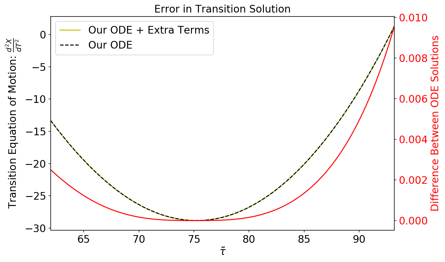
Notice here that this ensures that the energy flux obeys and is thus not constant. This ensures that we are still granted a full cancellation of the dissipative part of the forcing term in Eq.(28). This will yield a continuous evolution at the matching point with a discontinuous first derivative. At this point we will have a full trajectory with (continuous) integrals of motion in proper time and . In each of 2000PhRvD..62l4022O; Transition_Inspiral_Scott_Hughes; sundararajan2008transition, the authors compute three separate worldlines in proper time; Adiabatic inspiral, transition, geodesic plunge. Apte et al in Transition_Inspiral_Scott_Hughes, provide an algorithm in which they freeze the constants of motion and when the extra terms in Eq.(64) exceed the leading order terms and by 5%. As one would expect, as one ventures farther from the ISCO, the Taylor expansion used to derive these transition equations of motion will break down. As such, it is very natural for each of the aforementioned authors to compute a geodesic plunge to complete their worldlines in proper time . Simply because, for moderate spins (non near-extremal), . For near-extreme black holes the ISCO is close to the horizon in Boyer Lindquist coordinates . The scaling of the near-extremal transition zone is also and so the horizon is reached while the object is still in the transition zone. We therefore do not expect to need to add a geodesic plunge to compute full near-extremal inspirals. To verify this we numerically calculate the extra terms in (100), which are
| (104) | ||||
We compare the solution to (100) when these terms are omitted or included in Figure 3. The difference is at most even the horizon . We conclude that we can use the solution from (100) throughout the plunging regime, for . It would be useful in the future to compare our results with the analytic geodesic plunges found in compere2018_NHEK.
IV.2 Worldline in Boyer-Lindquist Coordinates
In the previous section, we computed the full worldline comprised of inspiral, transition and plunge parametrized as . We now intend to do the same but in coordinate time so that our worldline is in Boyer-Lindquist coordinates . Loosely speaking, this is the time measured from Earth (at radial infinity) so is useful for observable purposes.
For the quasi-circular inspiral solution, we simply integrate the circular relation relating coordinate time to proper time via Eq.(8)
| (105) |
where is the worldline constructed by integrating Eq.(99) up to some suitable point to begin the transition solution, in our case, . To compute the trajectory in coordinate time throughout the transition regime, we must integrate
| (106) |
where is given by 4 and is defined through . Throughout the transition regime, we use the model for both and given by Eq.(103) and Eq.(102). This will yield the throughout the transition regime. Combining these results yield a full trajectory from radial infinity to the horizon in coordinate time .
To then calculate the orbital velocity in coordinate time we substitute found previously into Eq.(9). This now gives valid throughout the adiabatic inspiral regime. Using our solutions for and defined through Eq.(102) and Eq.(103) and throughout the transition regime, we calculate
| (107) |
where . This algorithm will provide a worldline in coordinate time which will be used for our waveforms. We stress here that is continuous and (once) differentiable.

IV.3 Near-Extremal Waveform
Following 2000PhRvD..62l4021F, the root mean square (rms) amplitude of gravitational waves emitted towards infinity at harmonic is given by . The plus and cross each represent individual transverse-traceless polarisations of the gravitational wave strain . The amplitudes are averaged over the direction and over the period of the waves. Furthermore, the rms amplitude generated by a particle on an equatorial circular orbit in the limit is related to the outgoing radiation flux in harmonic by
| (108) |
for distance and outgoing fluxes defined by
| (109) |
where the amplitude equals
and is the relativistic correction to at each harmonic .
An EMRI signal is a superposition of infinitely many harmonics of the fundamental frequency
| (110) |
with . Recall that the total emission of radiation through gravitational waves is related to the outgoing and ingoing flux by
| (111) | ||||
where is the ingoing flux (towards the horizon) including the contribution from all for each harmonic . Using the exact results from the BHPT for a spin parameter of , we constructed a cubic spline for each outgoing flux . Our results are plotted in figure 5. It is clear that including the higher order modes become increasingly important as the spin parameter increases towards unity. This has already been observed in compere2018_NHEK. Hence, for near-extremal systems, only using the harmonic is not an accurate representation of the EMRI signal in general.

Figure 5 suggests that truncating the sum at the eleventh harmonic in the outgoing flux (111) is a good approximation to model a near-extremal waveform encapsulating quasi-circular inspiral, transition, and then plunge with suitable accuracy. The remaining difference from modes with contributes a small difference in the amplitude of the waveform, but gravitational wave detectors are much less sensitive to amplitude corrections than corrections to the phase. The phase evolution is determined by the total flux, in which we are including all modes. We therefore believe that the approximate waveform with modes is a sufficiently accurate model for parameter estimation studies and will use this henceforth
| (112) |
Once the ISCO is reached, we smoothly extrapolate each of the fluxes , as . This is a similar approach to that found in Taracchini et al in Small_Mass_Plunging. Using (112) and the results obtained in this paper, we plot a near-extremal waveform, including the transition from inspiral to plunge, in Fig.(6).


We notice that the waveform in Figure 6 exhibits the usual dampening before the ISCO is reached as seen by Gralla et al in 2016CQGra..33o5002G. This, qualitatively, is a unique feature to near-extreme EMRIs as a gravitational wave source.
V Conclusion
This paper has presented a solution to the problem of the transition from inspiral to plunge, for any primary spin, for EMRIs on circular and equatorial orbits. This work has extended the treatment of Ori & Thorne 2000PhRvD..62l4022O which was the first analysis of this problem but did not apply to systems with near-extremal spins. This work also extended the analysis of kesden2011transition which did consider near extremal spins, by providing a better physical interpretation of the procedure, identifying a missing term in the analysis and updating the treatment to use recent calculations of the near-extremal energy flux. We have also carefully identified the scaling of the various higher order terms arising from effects such as eccentricity and non-geodesic past-history to carefully demonstrate that these are all sub-dominant. Previous treatments have assumed that the quasi-circular assumption holds throughout the inspiral, but without rigorous justification. We have demonstrated that initial eccentricities excited during the adiabatic inspiral regime grow by the time the transition regime is reached, but are still sufficiently small to be sub-dominant. We have shown that corrections to the flux balance law (29) arising from eccentricity and from the non-geodesic past-history of the orbital evolution are also sub-dominant, if only marginally, but there are non-trivial deviations from the linear-in-proper-time evolution of energy and angular momentum in (36) that was assumed in OT. These deviations are encoded in the evolution of the parameter through the transition regime.
Based on these arguments, we have derived a transition equation for each of the three scaling regimes: , and and described a numerical scheme to generate a full inspiral trajectory in coordinate time, from radial infinity to the horizon. For near-extremal black holes, we found that there was no need to attach a geodesic plunge onto the transition solution as the inspiraling object reaches the horizon while still within the transition regime. Finally, we used these inspiral trajectories to construct a near-extremal waveform exhibiting the transition and plunging dynamics using results from the BHPT BHPToolkit.
The OT procedure is straightforward, but with surprisingly rich phenomenology. Through semi-analytic means, one is able to derive an equation which describes the dynamics within the vicinity of the ISCO. However, in practice, the OT theory has several shortcomings. The point at which the transition solution is taken to start has a significant influence on the time it takes the particle to reach the horizon and so the OT procedure does not define a unique worldline given a particular set of parameters for the source. This is clearly not physical behaviour. We argued in section IV.1 that if the switch from the adiabatic inspiral to the transition equation is made when the constraint is satisfied, the solution will be almost unique. This was verified numerically and we found it leads to plunge times consistent within . This very same problem was found in Transition_Inspiral_Scott_Hughes but they saw no effect in their waveform analysis. For the case, there is a further degree of freedom as to when to attach the geodesic plunge. To do so, one must “freeze” the integrals of motion at the end of the transition regime and integrate the Kerr geodesic equations forward in coordinate time. Attaching the geodesic plunge is discussed, at length, in Transition_Inspiral_Scott_Hughes but does not have a unique solution. Care must be taken as to when the transition solution and the geodesic plunge is attached or comparatively different radial trajectories will be produced. Fortunately for the case, there is no need to attach a geodesic plunge as shown earlier in section IV.1.
Another issue with the OT method is that it can lead to discontinuities in the constants of motion and if the OT equations are integrated backwards from the ISCO rather than forwards from the point of the switch from the adiabatic inspiral to transition regime. Discontinuities in the constants of motion lead to discontinuities in the coordinate time trajectories and in the waveforms which must be avoided if these waveforms are to give physically reasonable results in parameter estimation studies. Our solution, which was to integrate forward not backwards, yields continuous, but not first order differentiable, trajectories. The procedure described in Transition_Inspiral_Scott_Hughes provides both. For parameter estimation studies we only require continuity of and and first order differentiability of and so our procedure should be sufficient, although this should be examined more carefully.
There are natural extensions of this work. First, the waveforms constructed in this paper can be used to carry out a parameter estimation study to understand how well the parameters of near-extremal EMRIs can be measured with observations by LISA. Of particular interest is how well the spin can be determined, since the identification of an object that definitely has spin above the Thorne limit would be of profound significance. Second, our waveforms are missing the quasi-normal mode ringdown contribution. Hence, it would be very interesting to generate a full waveform taking these into account, together with the plunging dynamics discussed here. Details on how to construct the waveform including this effect were discussed in Yang:2013uba. Finally, it would also be of interest to extend the current analysis to inspirals that are not circular and equatorial. The extension of OT was first performed in sundararajan2008transition who attempted to solve the problem for generic orbits; both eccentric and inclined orbits. Sundararajan’s treatment was corrected by Transition_Inspiral_Scott_Hughes in the case of arbitrary inclination. Hence, no one, as of yet, has considered the transition from inspiral to plunge in the case of eccentric orbits and inclined orbits. These orbits are expected for EMRIs formed through standard astrophysical channels amaro2007intermediate. The extension to eccentric orbits will require more careful modelling of the self-force and the use of the (eccentricity-dependent) separatrix in place of the ISCO among other complications. A model of the transition for inspirals on generic orbits into black holes arbitrary spin will be invaluable for the analysis of future LISA EMRI observations and is an important future topic of study.
Acknowledgements.
This work made use of data hosted as part of the Black Hole Perturbation Toolkit at bhptoolkit.org. We wish to thank Maarten van de Meent for his comments on the final stages of this manuscript. We also give our thanks to Maarten for pointing out useful literature concerning the conservative part of the self-force and giving direction on why we could neglect it. We also wish to thank Niels Warburton for his guidance using the toolkit and Peter Zimmerman for his useful discussions regarding the behaviour of near-extremal Kerr Black holes. Finally, we thank Geoffrey Compère for comments on an earlier version of this manuscript.Appendix A The Innermost Stable Circular Orbit
In this appendix we review the main properties of the function determining the radial geodesic (2)
| (113) | ||||
together with its derivatives when evaluated at the ISCO orbit . The spin dependence of these quantities will play a critical role in the identification of the different transition regimes discussed in section III.
Remember the ISCO radial coordinate is characterised by marginal stability
| (114) |
Labelling the energy and angular momentum of the ISCO orbit by and , we can solve the second and third constraint equations by
| (115) | ||||
Plugging these into , one derives the relation
| (116) |
which combined with (115) yields
| (117) |
whose solution reproduces (14) 1972ApJ…178..347B. This equality allows to simplify the energy (5) and angular momentum (6) of equatorial circular orbits when evaluated at ISCO to
| (118) | ||||
| (119) |
Armed with these identities, we move towards the evaluation of the derivatives controlling the expansions (38) relevant to the transition regime. First, we introduce some notation
| (120) | ||||
with as in(9). Either by explicit calculation or by induction, one can prove for any integer
where for and zero otherwise. Finally, evaluating these derivatives at and using the properties (114)-(119), we can derive the exact results
| (121) | |||||
| (122) | |||||
| (123) |
Notice equations (121)-(122) recover the familiar identities for circular orbits
Let us study the behaviour of these derivatives for near extremal black holes, i.e. in the limit as introduced in section II. Remember is given by
| (124) |
Using this expansion together with , we can evaluate the leading terms of all previous derivatives to be
| (125) | ||||
| (126) | ||||
| (127) | ||||
| (128) | ||||
| (129) | ||||
| (130) |
where we defined
| (131) |
Appendix B Retrograde Orbits
In this section, we will restrict our attention to retrograde orbits. That is, orbits opposing the direction with the primaries angular momenta. These orbits are of interest because the ISCO is much further away from the horizon, which implies that the radial distance travelled during plunge time is much longer. We plot the location of the ISCO as a function of spin in figure (7).

Due to frame-dragging, we expect the ISCO to be farther from the hole since the space is dragged in the opposite direction to the compact objects orbital direction. In our conventions, retrograde orbits correspond to and . Hence, near-extremal ones are characterised by , or equivalently, by
| (132) |
notice that the horizon takes the same form as in the case of prograde orbits
as to be expected. Using a spin parameter of negative parity, the expressions for and remain the same. However, each quantity will be different at the ISCO of a retrograde orbit. By substituting Eq. (132) into Eqs.(6), (5), (14) and (9) for small , one finds
| (133) | ||||
| (134) | ||||
| (135) | ||||
| (136) |
Notice here that the expansion in is no longer increasing in powers of and now in . Also notice that rather than of order like in the case of near-extremal prograde orbits. Like we have done previously, we consider the Kerr radial velocity expanded around the ISCO
| (137) |
with small variables
| (138) | ||||
| (139) | ||||
| (140) |
The coeffcients in (137) can be approximated for under the retrograde condition Eq.(132)
and in (137) defined through equation (41). Notice that none of the coefficients in our transition equation of motion depend on the extremality parameter . This gives us no reason to introduce any scalings on and like we did for prograde orbits around rapdily rotating black holes. As such, let us introduce similar scalings to OT
| (141) | ||||
| (142) | ||||
| (143) | ||||
| (144) |
Substituting these results into Eq.(137) we find that
| (145) |
Since , we only need the first term of
| (146) |
and taking derivatives of Eq.(145) and following an identical procedure to subsection (III.4),
| (147) |
with evolution equation for
| (148) |
for . Which is precisely the equation of motion for the transition regime derived by OT in 2000PhRvD..62l4022O. Although the quantities and present in the change of coordinates are different, the physics and ultimate end goal are the same. As a result, we stop our analysis of retrograde orbits here since we feel that this problem has already been solved by the community for smaller spin values . We conclude that, for near-extremal retrograde orbits, there is nothing new to learn about the transition regime. It can be solved in the matter of OT in 2000PhRvD..62l4022O. We do remark that the quantity can no longer be computed using the near-extremal formula defined by . This is because the transition region is far from the horizon of the primary hole [see figure (1)]. Instead we have to use the numerical quantity
Various results are tabulated (including retrograde orbits) in 2000PhRvD..62l4021F. The downside of this equation is that it can only be evaluated numerically.
Appendix C Osculating Elements Equations
The proper time derivative of the radial geodesic equation (2) yields (26)
| (149) |
The purpose of this appendix is to review how this equation is equivalent to the radial component of a forced geodesic equation
| (150) |
where , , is the four-velocity of the particle and a forcing term driving deviations from geodesic motion.
To show the equivalence between (149) and (150), we use the osculating elements formulation pound2008osculating. Since this method does not take into account conservative effects arising from the self-force barack2018self, the component in this appendix will only account for the dissipative piece in (28). Its conservative piece is treated in more detail in the main text (See section III.1).
Since the four velocity is normalised, it follows is normal to it by proper time differentiation
| (151) |
Evaluating (150) along the radial direction, solving (151) for and plugging it into (150) yields
| (152) |
The left hand side
| (153) |
is computed using the Kerr Christoffel symbols and the geodesic equations (2)-(4)
To evaluate the right hand side, , we first notice the existence of two Killing vectors : and , associated with time and angular translational invariance, respectively. There exists a conserved charge associated with each :
| (154) |
It follows from Eq.(154) that and . Finally, we relate the proper time derivatives of these charges with the forcing terms in (150). For example, consider the proper time derivative of
| (155) | ||||
where Killing’s equation was used in the last step. A similar calculation leads to . Solving the two equations and for and gives
where we used the identity for . Since , it follows the right hand side of (152) is
Noticing that
| (156) | ||||
| (157) |
we reach the desired conclusion
| (158) |
References
- (1) B. P. e. a. Abbott, “Observation of gravitational waves from a binary black hole merger,” Phys. Rev. Lett., vol. 116, p. 061102, Feb 2016. [Online]. Available: https://link.aps.org/doi/10.1103/PhysRevLett.116.061102
- (2) L. Scientific, “Gwtc-1: A gravitational-wave transient catalog of compact binary mergers observed by ligo and virgo during the first and second observing runs,” arXiv preprint arXiv:1811.12907, vol. 2, 1811.
- (3) T. Baker, E. Bellini, P. G. Ferreira, M. Lagos, J. Noller, and I. Sawicki, “Strong constraints on cosmological gravity from gw170817 and grb 170817a,” Physical review letters, vol. 119, no. 25, p. 251301, 2017.
- (4) D. Langlois, R. Saito, D. Yamauchi, and K. Noui, “Scalar-tensor theories and modified gravity in the wake of gw170817,” Phys. Rev. D, vol. 97, no. 6, p. 061501, 2018.
- (5) J. M. Ezquiaga and M. Zumalacárregui, “Dark energy after gw170817: dead ends and the road ahead,” Physical review letters, vol. 119, no. 25, p. 251304, 2017.
- (6) J. Sakstein and B. Jain, “Implications of the neutron star merger gw170817 for cosmological scalar-tensor theories,” Physical review letters, vol. 119, no. 25, p. 251303, 2017.
- (7) S. Boran, S. Desai, E. Kahya, and R. Woodard, “Gw170817 falsifies dark matter emulators,” Phys. Rev. D, vol. 97, no. 4, p. 041501, 2018.
- (8) B. S. Sathyaprakash and B. F. Schutz, “Physics, astrophysics and cosmology with gravitational waves,” Living reviews in relativity, vol. 12, no. 1, p. 2, 2009.
- (9) D. J. Croton, V. Springel, S. D. White, G. De Lucia, C. S. Frenk, L. Gao, A. Jenkins, G. Kauffmann, J. Navarro, and N. Yoshida, “The many lives of active galactic nuclei: cooling flows, black holes and the luminosities and colours of galaxies,” Monthly Notices of the Royal Astronomical Society, vol. 365, no. 1, pp. 11–28, 2006.
- (10) P. Amaro-Seoane et al., “Laser Interferometer Space Antenna,” ArXiv e-prints, Feb. 2017.
- (11) P. Amaro-Seoane, J. R. Gair, M. Freitag, M. C. Miller, I. Mandel, C. J. Cutler, and S. Babak, “Intermediate and extreme mass-ratio inspirals—astrophysics, science applications and detection using lisa,” Classical and Quantum Gravity, vol. 24, no. 17, p. R113, 2007.
- (12) A. Sesana, E. Barausse, M. Dotti, and E. M. Rossi, “Linking the Spin Evolution of Massive Black Holes to Galaxy Kinematics,” Astrophys. J. , vol. 794, no. 2, p. 104, Oct 2014.
- (13) K. S. Thorne, “Disk-Accretion onto a Black Hole. II. Evolution of the Hole,” apj, vol. 191, pp. 507–520, Jul. 1974.
- (14) A. Arbey, J. Auffinger, and J. Silk, “Any extremal black holes are primordial,” arXiv preprint arXiv:1906.04196, 2019.
- (15) J. M. Bardeen and G. T. Horowitz, “The Extreme Kerr throat geometry: A Vacuum analog of AdS(2) x S**2,” Phys. Rev., vol. D60, p. 104030, 1999.
- (16) H. K. Kunduri, J. Lucietti, and H. S. Reall, “Near-horizon symmetries of extremal black holes,” Class. Quant. Grav., vol. 24, pp. 4169–4190, 2007.
- (17) A. P. Porfyriadis and A. Strominger, “Gravity waves from the Kerr/CFT correspondence,” Phys. Rev., vol. D90, no. 4, p. 044038, 2014.
- (18) S. Hadar, A. P. Porfyriadis, and A. Strominger, “Gravity Waves from Extreme-Mass-Ratio Plunges into Kerr Black Holes,” Phys. Rev., vol. D90, no. 6, p. 064045, 2014.
- (19) ——, “Fast plunges into Kerr black holes,” JHEP, vol. 07, p. 078, 2015.
- (20) S. E. Gralla, A. P. Porfyriadis, and N. Warburton, “Particle on the innermost stable circular orbit of a rapidly spinning black hole,” prd, vol. 92, no. 6, p. 064029, Sep. 2015.
- (21) M. H. Van Putten, “Near-extremal black holes as initial conditions of long grb supernovae and probes of their gravitational wave emission,” The Astrophysical Journal, vol. 810, no. 1, p. 7, 2015.
- (22) S. Hadar and A. P. Porfyriadis, “Whirling orbits around twirling black holes from conformal symmetry,” JHEP, vol. 03, p. 014, 2017.
- (23) S. E. Gralla, S. A. Hughes, and N. Warburton, “Inspiral into Gargantua,” Classical and Quantum Gravity, vol. 33, no. 15, p. 155002, Aug. 2016.
- (24) K. Chatziioannou, G. Lovelace, M. Boyle, M. Giesler, D. A. Hemberger, R. Katebi, L. E. Kidder, H. P. Pfeiffer, M. A. Scheel, and B. Szilágyi, “Measuring the properties of nearly extremal black holes with gravitational waves,” ArXiv e-prints, Apr. 2018.
- (25) G. Compère, K. Fransen, T. Hertog, and J. Long, “Gravitational waves from plunges into gargantua,” Classical and Quantum Gravity, vol. 35, no. 10, p. 104002, 2018.
- (26) D. Kapec and A. Lupsasca, “Particle motion near high-spin black holes,” arXiv preprint arXiv:1905.11406, 2019.
- (27) A. Ori and K. S. Thorne, “Transition from inspiral to plunge for a compact body in a circular equatorial orbit around a massive, spinning black hole,” prd, vol. 62, no. 12, p. 124022, Dec. 2000.
- (28) A. Buonanno and T. Damour, “Transition from inspiral to plunge in binary black hole coalescences,” Physical Review D, vol. 62, no. 6, p. 064015, 2000.
- (29) M. Kesden, “Transition from adiabatic inspiral to plunge into a spinning black hole,” Phys. Rev. D, vol. 83, no. 10, p. 104011, 2011.
- (30) P. A. Sundararajan, “Transition from adiabatic inspiral to geodesic plunge for a compact object around a massive kerr black hole: Generic orbits,” Phys. Rev. D, vol. 77, no. 12, p. 124050, 2008.
- (31) A. Apte and S. A. Hughes, “Exciting black hole modes via misaligned coalescences: I. inspiral, transition, and plunge trajectories using a generalized ori-thorne procedure,” arXiv preprint arXiv:1901.05901, 2019.
- (32) G. Compère, K. Fransen, and C. Jonas, “Transition from inspiral to plunge into a highly spinning black hole,” arXiv e-prints, p. arXiv:1909.12848, Sep 2019.
- (33) W. Schmidt, “Celestial mechanics in Kerr space-time,” Class. Quant. Grav., vol. 19, p. 2743, 2002.
- (34) S. Chandrasekhar, The mathematical theory of black holes, ser. Oxford classic texts in the physical sciences. Oxford: Oxford Univ. Press, 2002. [Online]. Available: https://cds.cern.ch/record/579245
- (35) D. Kennefick, “Stability under radiation reaction of circular equatorial orbits around Kerr black holes,” Phys. Rev. D, vol. 58, no. 6, p. 064012, Sep 1998.
- (36) J. M. Bardeen, W. H. Press, and S. A. Teukolsky, “Rotating black holes: locally nonrotating frames, energy extraction, and scalar synchrotron radiation,” The Astrophysical Journal, vol. 178, pp. 347–370, 1972.
- (37) S. A. Teukolsky, “Perturbations of a Rotating Black Hole. I. Fundamental Equations for Gravitational, Electromagnetic, and Neutrino-Field Perturbations,” Astrophys. J., vol. 185, pp. 635–648, Oct. 1973.
- (38) M. Sasaki and T. Nakamura, “Gravitational Radiation from a Kerr Black Hole. I —Formulation and a Method for Numerical Analysis—,” Progress of Theoretical Physics, vol. 67, pp. 1788–1809, Jun. 1982.
- (39) S. A. Hughes, “Evolution of circular, nonequatorial orbits of Kerr black holes due to gravitational-wave emission,” Phys. Rev. D, vol. 61, no. 8, p. 084004, Mar 2000.
- (40) K. Glampedakis and D. Kennefick, “Zoom and whirl: Eccentric equatorial orbits around spinning black holes and their evolution under gravitational radiation reaction,” Phys. Rev. D, vol. 66, no. 4, p. 044002, Aug 2002.
- (41) S. Drasco and S. A. Hughes, “Gravitational wave snapshots of generic extreme mass ratio inspirals,” Phys. Rev. D, vol. 73, p. 024027, 2006.
- (42) L. S. Finn and K. S. Thorne, “Gravitational waves from a compact star in a circular, inspiral orbit, in the equatorial plane of a massive, spinning black hole, as observed by LISA,” prd, vol. 62, no. 12, p. 124021, Dec. 2000.
- (43) P. Peters and J. Mathews, “Gravitational radiation from point masses in a keplerian orbit,” Physical Review, vol. 131, no. 1, p. 435, 1963.
- (44) T. Apostolatos, D. Kennefick, A. Ori, and E. Poisson, “Gravitational radiation from a particle in circular orbit around a black hole. iii. stability of circular orbits under radiation reaction,” Phys. Rev. D, vol. 47, no. 12, p. 5376, 1993.
- (45) Y. Mino, “Perturbative approach to an orbital evolution around a supermassive black hole,” Phys. Rev., vol. D67, p. 084027, 2003.
- (46) L. Barack and A. Pound, “Self-force and radiation reaction in general relativity,” Reports on Progress in Physics, vol. 82, no. 1, p. 016904, 2018.
- (47) L. Barack and N. Sago, “Gravitational self-force correction to the innermost stable circular orbit of a schwarzschild black hole,” Physical review letters, vol. 102, no. 19, p. 191101, 2009.
- (48) M. Van De Meent, “Self-force corrections to the periapsis advance around a spinning black hole,” Physical review letters, vol. 118, no. 1, p. 011101, 2017.
- (49) S. Isoyama, L. Barack, S. R. Dolan, A. Le Tiec, H. Nakano, A. G. Shah, T. Tanaka, and N. Warburton, “Gravitational self-force correction to the innermost stable circular equatorial orbit of a kerr black hole,” Physical review letters, vol. 113, no. 16, p. 161101, 2014.
- (50) D. Kennefick and A. Ori, “Radiation reaction induced evolution of circular orbits of particles around Kerr black holes,” Phys. Rev., vol. D53, pp. 4319–4326, 1996.
- (51) E. Poisson, A. Pound, and I. Vega, “The motion of point particles in curved spacetime,” ArXiv e-prints, Feb. 2011.
- (52) J. M. Bardeen, W. H. Press, and S. A. Teukolsky, “Rotating Black Holes: Locally Nonrotating Frames, Energy Extraction, and Scalar Synchrotron Radiation,” apj, vol. 178, pp. 347–370, Dec. 1972.
- (53) T. Jacobson, “Where is the extremal Kerr ISCO?” Class. Quant. Grav., vol. 28, p. 187001, 2011.
- (54) S. E. Gralla, A. P. Porfyriadis, and N. Warburton, “Particle on the Innermost Stable Circular Orbit of a Rapidly Spinning Black Hole,” Phys. Rev., vol. D92, no. 6, p. 064029, 2015.
- (55) A. Taracchini, A. Buonanno, G. Khanna, and S. A. Hughes, “Small mass plunging into a Kerr black hole: Anatomy of the inspiral-merger-ringdown waveforms,” prd, vol. 90, no. 8, p. 084025, Oct 2014.
- (56) “Black Hole Perturbation Toolkit,” bhptoolkit.org.
- (57) H. Yang, A. Zimmerman, A. Zenginoğlu, F. Zhang, E. Berti, and Y. Chen, “Quasinormal modes of nearly extremal Kerr spacetimes: spectrum bifurcation and power-law ringdown,” Phys. Rev., vol. D88, no. 4, p. 044047, 2013, [Phys. Rev.D88,044047(2013)].
- (58) A. Pound and E. Poisson, “Osculating orbits in schwarzschild spacetime, with an application to extreme mass-ratio inspirals,” Phys. Rev. D, vol. 77, no. 4, p. 044013, 2008.