Stochastic Effects in Anisotropic Inflation
Alireza Talebian1 ** * talebian@ipm.ir, Amin Nassiri-Rad1 †† † amin.nassiriraad@ipm.ir, Hassan Firouzjahi1,2 ‡‡ ‡ firouz@ipm.ir,
1School of Astronomy, Institute for Research in Fundamental Sciences (IPM)
P. O. Box 19395-5531, Tehran, Iran
2 Department of Physics, Faculty of Basic Sciences, University of Mazandaran,
P. O. Box 47416-95447, Babolsar, Iran
Abstract
We revisit the stochastic effects in the model of anisotropic inflation containing a gauge field. We obtain the Langevin equations for the inflaton and gauge fields perturbations and solve them analytically. We show that if the initial value of the electric field is larger than its classical attractor value, then the random stochastic forces associated with the gauge field is balanced by the frictional damping (classical) force and the electric field falls into a equilibrium (stationary) regime. As a result, the classical attractor value of the electric field is replaced by its stationary value. We show that the probability of generating quadrupolar statistical anisotropy consistent with CMB constraints can be significant.
1 Introduction
Thanks to numerous cosmological observations, inflationary cosmology has emerged as the leading paradigm for the early universe cosmology. In its simplest realization, inflation is driven by a scalar field, the inflaton field, which slowly rolls overs its flat potential. The quantum fluctuations of the inflaton field, stretched over the horizon of a near de-Sitter background, is the origin of the Cosmic Microwave Background (CMB) temperature anisotropies and the seeds of the large scale structure. The statistical features of these fluctuations are well consistent with the basic predictions of simple inflationary scenarios where the primordial perturbations are observed to be nearly scale invariant, adiabatic and almost Gaussian [1, 2].
Although a statistically isotropic universe is well supported by the CMB observations, but the possibility of having “anisotropic hair” in the early universe has attracted considerable interests in recent years. The simplest mechanism to generate statistical anisotropies on large scales is based on the so called model of in which a gauge field is non-minimally coupled to the inflaton field via the conformal coupling . With an appropriate choice of the conformal coupling, the energy is dragged continuously from the inflaton background to the gauge field sector such that the background electric field survives the exponential expansion while a nearly scale invariant gauge field perturbations can be generated on superhorizon scales [3]. The basic prediction of models of anisotropic inflation is that a quadrupolar type statistical anisotropy is generated on CMB maps. However, there are strong observational bounds on the amplitude of quadrupolar statistical anisotropy, [4, 5], which poses strong constraint on the parameters of the models of anisotropic inflation. For various works related to anisotropic inflation see [3, 6, 7, 8, 9, 10, 11, 12].
In order to meet the observational bounds on , the contributions of the background electric field to the total energy must be kept under control. The energy density of the gauge field settles to an attractor value via the back-reaction mechanism [3]. Independent of the initial value of the background electric field energy density, the back-reactions between the gauge field and the inflaton field drive the system to its attractor regime in which the electric field energy density is a small but a nearly constant fraction of the total energy density. However, this is the classical picture in which the stochastic effects of the short wavelength perturbations are neglected. One might worry that the effects of short-wavelength perturbations can significantly influence the background dynamics, preventing the system from reaching to its attractor solution [13]. One of the well known approach to study quantum effects of these modes during inflation is the stochastic inflation formalism [14, 15, 16, 17, 18, 19, 20, 21, 22, 23, 24, 25, 26, 27, 28, 29, 30, 31, 32, 33, 34, 35, 36, 37, 38, 39, 40, 41, 42, 43, 44, 45, 13, 46, 47, 48, 49]. In this approach, the quantum fluctuations are decomposed into the infrared (IR) and ultraviolet (UV) modes. As the UV modes are stretched and leaving the Hubble horizon during inflation, they act as quantum kicks on super-horizon scale perturbations (classical solutions) with the amplitude in which is Hubble expansion rate during inflation. These quantum noises can be translated into a stochastic force imposed on the classical slow-roll dynamics of the coarse grained IR modes. Consequently, the deterministic interpretation of the dynamics of the field on large scale is replaced by a probabilistic one.
Fujita and Obata [13] have studied the stochastic effects of the gauge fields perturbations in the model of anisotropic inflation. They derived the Langevin and the Fokker-Planck equations for the gauge fields perturbations and showed that the gauge field fluctuations pile up and quickly overwhelm the classical attractor solution. By assuming that the gauge field is in the stochastic equilibrium when the CMB modes exit the horizon, they reported that the probability of the CMB statistical anisotropy to be consistent with the current observational upper bound is around 0.001%, excluding anisotropic inflation scenario with the probability about 99.999%. It is argued that this conclusion is independent of the model parameters or the initial conditions.
In this paper we revisit the stochastic effects of the gauge field and the inflaton field in anisotropic inflation model and derive the associated Langevin equations. Some of our results disagree with those of [13]. In particular, we show that the fate of electric field is sensitive to its initial value relative to the classical attractor value . If , the stochastic effects of the electric field become relevant only after an exponentially large number of e-folds has passed. However, for , the accumulative effects of the stochastic noises are not strong enough to spoil the nearly-isotropic approximation of setup and the classical attractor mechanism of [3] is reached. In this case the system falls into a equilibrium state where the stochastic and classical forces balance each other.
The paper is organized as follows. In Sec. 2, the model of anisotropic inflation and its predictions for statistical anisotropy are reviewed. The Langevin equation of the electric field is derived in Sec. 3 and the effects of quantum kicks on the coarse-grained electric field are studied in three subclasses. In Sec. 4, the stochastic dynamics of the inflaton field are studied followed by the summaries and discussions in Sec. 5. The derivations of the correlation functions of the electric and magnetic noises and a brief review of the probability distribution function are presented in appendices A and B, respectively.
2 Anisotropic Inflation
Here we review the setup of anisotropic inflation and collect the necessary results for the stochastic analysis in next Sections. The model contains the inflaton field which is a real scalar field coupled to an Abelian gauge field through the gauge kinetic coupling via the following action
| (1) |
in which is the reduced Planck mass, is the field strength associated with the gauge field and is the Ricci scalar. The background metric is in the form of the Bianchi type I universe,
| (2) |
Here is the number of -folds so represents the Hubble expansion rate, where a dot denotes the derivative with respective to . Without loss of generality, we can align the -axis along the direction of the background vector field, , and consider the axisymmetric line element matrix as
| (3) |
where measures the anisotropy expansion rate. Observationally, the deviation from isotropy is very small, therefore we demand that the quantity measuring the fractional anisotropic expansion to be very small, .
Going to Coulomb-radiation gauge , the equations of motion for the inflaton and gauge fields respectively are
| (4) | |||
| (5) |
Hereafter, the bold symbols denote vector quantities. Associated with the gauge field , we can define the electric field and the magnetic field , where their magnitudes appear in Eq. (4). Since the background is homogeneous, so the energy density of the gauge field is given by the electric field,
| (6) |
Moreover, the Einstein field equations are given by
| (7) | |||||
| (8) | |||||
| (9) |
The total energy density governing the dynamics of inflation is given by the right hand side of Eq. (7) in which the last term comes from the gauge field. In order to have a long period of slow-roll inflation, we require that
| (10) |
In order to have small anisotropy, the electric field energy density should be small compared to the inflaton energy density . Defining the parameter as the fraction of the electric field energy density to the inflaton energy density,
| (11) |
we require that .
As seen from Eq. (9), the fate of the anisotropy expansion rate depends on the behavior of gauge field energy density. For a homogeneous gauge field satisfying the Maxwell equation (5), the electric field energy density is given by
| (12) |
where is a constant of integration. In the critical case with , and neglecting the anisotropy , the electric field energy density remains constant and no anisotropy is produced during inflation. At the level of perturbations, this critical case corresponds to the situation where the gauge field perturbations become pure isocurvature, with no contribution to primordial power spectrum.
More generally, choosing the conformal coupling in the form,
| (13) |
with being a model parameter, it is shown in [3] that the system reaches the attractor regime in which the electric field energy density furnishes a small but a constant fraction of the total energy density. More specifically, it is shown in [3] that
| (14) |
where and is the slow-roll parameter.
In this limit the kinetic coupling function can be obtained as [3]
| (15) |
where is an integration constant. Furthermore, the background electric field energy density as a function of time is given by [3]
| (16) |
Consequently can be determined by the initial value of , e.g. consider when ; then is given by
| (17) |
This can also be rewritten as
| (18) |
where
| (19) |
In general, when the system is not in its attractor regime, one can extend Eq. (14) to the following form
| (20) |
It was argued in [3] that as the background expands the term containing in the denominator of Eq. (16) falls off exponentially. Therefore, waiting long enough, one can neglect the term containing in , yielding to the attractor solution . Typically, one expects this happens after e-folds. However, as we shall see later, from the observational constraint on the amplitude of quadrupole anisotropy one requires that . This means that in order for the system to reach the attractor regime, one has to wait for about e-folds. It was argued in [13] that during this long period, the stochastic effects of the gauge field perturbations will build up and prevent the system from reaching to its final attractor regime. The issue of whether or not the system will reach to its attractor phase and its observational implications were also studied in [11]. One of the main goal of this paper is to study the roles of stochastic effects more systematically.
Next, we review the statistical properties of the curvature perturbations in this model. Since the dominant contributions in statistical anisotropies come from the matter fields perturbations, one can neglect the gravitational back-reactions including the effects of in the metric [9]. First, we look at the evolution of the gauge field perturbation which, in Fourier space, can be expanded as
| (21) |
Here is the conformal time and and are the annihilation and creation operators, respectively, satisfying the commutation relation,
| (22) |
Also represents the circular polarization vectors, normalized such that
| (23) | |||||
| (24) | |||||
| (25) | |||||
| (26) | |||||
| (27) |
Assuming with from Eq. (13), and starting with the Bunch-Davies (Minkowski) initial condition, the electric and magnetic components of the gauge field perturbations on super-horizon limit are given by [8]
| (28) |
As we mentioned before, for the critical case with corresponding to , the electric field perturbations are frozen on super-horizon scales, behaving as pure isocurvature perturbations. In the general case where with , the electric field perturbations contribute to the power spectrum of curvature perturbation, , yielding the correction in power spectrum [7, 8, 9, 10],
| (29) |
where is the preferred anisotropic direction in the sky (the -axis in our example), is the number of e-folds when the mode of interest leaves the horizon and represents the isotropic power spectrum,
| (30) |
Comparing the total power spectrum with the quadrupolar anisotropic estimator defined by
| (31) |
we obtain
| (32) |
To solve the flatness and the horizon problems, we need at least for the CMB scale modes. Also, from cosmological observations, we have [2, 5]. Therefore, if the system had been in the attractor regime till , the background electric field energy density was given by its attractor value and we obtain the following constraint on anisotropy parameter,
| (33) |
The problem with this small upper bound on is that it takes the system a long period of inflation to reach to its attractor regime. Specifically, as mentioned before, in order for the system to reach the attractor regime one has to neglect the effects of the term containing the parameter in the denominator of Eq. (16). This is justified if one waits e-folds of inflation. It is natural to expect that the stochastic effects of the gauge field perturbations may build up during this long period of inflation, spoiling the validity of the attractor assumption [13]. We study this question more systematically in next Sections.
3 Stochastic Effects of Gauge Fields
In this Section we study the stochastic effects of the gauge fields on the would-be attractor solution of [3].
The profile of the electric and the magnetic perturbations on superhorizon scales are given in Eq. (28). As seen, with , the electric field does not decay on superhorizon scales while the magnetic field falls off exponentially so we study the electric field perturbations.
The equation of motion for the electric field components is given by
| (34) |
To employ the stochastic formalism, we decompose the fields and their conjugate momenta into the UV and the IR parts. We are interested in the dynamics of the IR modes which are affected by the UV modes. The quantum fluctuations of the UV modes are represented by a Gaussian white noise, of which its amplitude is determined by the Hubble expansion rate during inflation.
With this discussion in mind, the electric field and its momentum are decomposed in IR and UV modes as follows:
| (35) | |||||
| (36) |
The UV parts are accompanied by a factor to exhibit the quantum nature of the short modes. The above decomposition is usually performed through an appropriate window function. Here we employ the Heaviside function to separate the long and short modes in which is a dimensionless parameter satisfying . Putting these together, we have
| (37) | |||||
| (38) | |||||
| (39) |
Here is the mode function which satisfies the following equation,
| (40) |
where we have assumed .
Imposing the Bunch-Davies (Minkowski) initial condition for the canonically normalized field when the modes are deep inside the horizon , we obtain the following solution for the electric field mode function,
| (41) |
Using the small argument limit of the Hankel function,
| (42) |
we see that for the electric field has the near scale invariant amplitude on superhorizon scales ,
| (43) |
Before continuing, it is instructive to compare the stochastic evolution of the electric field energy density with the classical one. The stochastic kicks from the vacuum fluctuations on the electric field energy density during one e-fold can be estimated as,
| (44) |
where is the dimensionless power spectrum of the electric field fluctuations in the super-horizon limit,
| (45) |
On the other hand, the classical evolution of during one e-fold can be estimated from Eq. (16) as
| (46) |
Hence the ratio of the classical evolution to the stochastic one is given by
| (47) |
where we have used and defined the following dimensionless parameters and ,
| (48) |
Note that from the constraint on , Eq. (33), we expect typically that . As seen in Fig.1, if , the stochastic kicks can not be ignored for . However, for the classical motion dominates and the system can reach to its classical attractor solution during one e-folding time. However, as we shall show below, for a general value of the accumulative effects of the stochastic noises can be relevant if an exponentially large number of e-folds has passed.

To consider the stochastic effects more systematically, following the logic of [16, 17, 18], we expand Eq. (34) around and and keep the terms up to first order of , obtaining
| (49) | |||||
| (50) |
in which and are the quantum noises, given by
| (51) | |||
| (52) |
In this view it is understood that the noise terms and behave as source terms originated from short modes which affect the evolution of long modes . The correlation functions of and in the Bunch-Davies vacuum are given by (see Appendix A for more details);
| (53) | |||||
| (54) | |||||
| (55) |
in which and is the zeroth order spherical Bessel function. In addition, the commutation relations of and are given by
| (56) | |||||
| (57) |
As it can be seen from Eqs. (56) and (57), the quantum nature of and disappears when is chosen small enough so one can treat them as classical noises. Therefore, on large-scale limit, we have (see App. A)
| (58) | |||||
| (59) |
Here we have replaced the time variable with the number of e-folds, , via .
One can combine Eqs. (49) and (50) in the slow-roll approximation where to obtain the corresponding Langevin equation for the superhorizon modes (where and ). For this purpose, let us first simplify the term inside the big bracket in Eq. (49). Noting that we work in the limit where and we have
| (60) |
in which we have defined the parameter via
| (61) |
Note that the parameter depends on the initial conditions through the parameter . In addition, from the definition of in Eq. (17) we have the lower bound . Also we work with , so the sign of the parameter is the same as .
Using the above approximations, Eqs. (49) and (50) can be combined to obtain the desired Langevin equation
| (62) |
The first term is called the “drift term” while the second one is the “diffusion term”. Here W is a three dimensional (3D) Wiener process [51] associated with a 3D normalized white classical noise defined via
| (63) | |||||
| (64) |
satisfying,
| (65) | |||||
| (66) |
By defining the following dimensionless stochastic variables,
| (67) |
the Langevin equation (62) can be cast into the form of a dimensionless stochastic differential equation
| (68) |
This is our master equation for the following analysis.
The general solution of Eq. (68) is given by
| (69) |
with the initial condition . The first term above represents the classical behavior of the electric field in the absence of stochastic noises,
| (70) |
As can be seen, the constant parameter plays crucial roles in stochastic differential equation Eq. (68). The definitions (18) and (67) help us to obtain the dependency of on initial condition as
| (71) |
We study the role of the parameter in more details below. But before doing so, let us calculate the expectation values (or mean values) and the variances related to vector stochastic quantity obtained in Eq. (69).
Using the following properties of the stochastic integrals [51]
| (72) |
we obtain
| (73) | |||||
| (74) | |||||
| (75) | |||||
| (76) | |||||
| (77) |
where the variance is defined via . We see that the above quantities depend on the number of e-fold and on the initial conditions via and .
Based on the above results, let us compare the case of the classical feedback mechanism with no quantum noises to the case when the stochastic effects are included. In the classical treatment where the contributions of the UV modes in electric energy density are neglected, the attractor regime is when approaches to unity. If , the back-reactions from electric field (the last term in Eq. (4) ) grows, reducing the inflaton velocity and suppressing . On the other hand, if , the inflaton velocity increases towards unity through the coupling . As a side remark, we note that switching off the feedback mechanism by going to the limit , stays on its initial value and there is no force to drive it to the attractor value.

However the story is very different when the stochastic noises are switched on. In Fig. 2 the numeric solution of Eq. (68) is plotted for different electric field initial conditions. As can be seen, the fate of electric field is somewhat sensitive to its initial value. If ), the system falls into a quasi-stable state (in the following we relate this quasi-stable state to the stationary solution of probability density function of electric field). The larger is , the faster the system falls into the quasi-stable state. On the other hand, for the electric field energy density grows continuously and there is no attractor regime. This is the non-trivial consequence of the stochastic effects of the gauge field perturbations.
One may worry that the accumulative effects of the stochastic noises may violate the condition required for a nearly isotropic background. Here we investigate this question while assuming that and rewrite the parameter in Eq. (48) for the IR part of dimensionless electric field as
| (78) |
For , and the initial electric field is somewhat larger (smaller) than the classical attractor value. The limit corresponds to the case where the system starts with its attractor value, , in which the Langevin equation (68) describes a pure Wiener process. Fig 3 presents the evolution of for . As can be seen, for , the nearly-isotropic slow-roll condition is never violated. However, for , the number of e-fold when approaches unity is in the range of . For a given value of , we have . Incidentally, note that this is also the number of e-folds required for the system to reach into its attractor limit in the classical picture of [3]. As a result, we conclude that the stochastic effects do not allow for the system to reach into its classical attractor limit when , i.e. when .

Moreover, equations (73)-(77) tell us that the sign of is very important in determining the fate of the electric field and inflation dynamics. To describe the time evolution of the probability density function of , we can employ the Fokker-Planck equation associated to the Langevin equation (62). The Fokker-Planck equation for the probability density of the random variable is given by
| (79) |
Intuitively, one can think of as being the probability of falling within the infinitesimal interval . The existence of a stationary solution for the probability density of the electric field (68) depends on the sign of , i.e. one must compare the initial electric energy density with its attractor value. In the following we have classified the model in three categories in the presence of stochastic noises.
3.1
If (i.e. the initial energy density of the electric field is smaller than its classical attractor value), the mean of the electric field energy density and its variance grow. At early stage when , the mean and the variance grow linearly with time,
| (80) | |||||
| (81) |
Although the classical contribution (70) is initially under control by the feedback mechanism, but when , the stochastic noises grows exponentially and spoil the feedback mechanism. Moreover, for , there is no stationary probability distribution and and grow linearly with time.
A spacial case is when so there is no classical energy density. In this case the system is described by a pure Brownian motion and . The linear growth of the variance with is the hallmark of the Brownian motion. We see that even with zero classical electric field energy density, the stochastic effects can grow and generate large electric field energy density.
3.2
If , the initial energy density of the electric field is equal to its classical attractor value and the Langevin equation (68) describes a Wiener process with no drift,
| (82) |
Correspondingly, the Fokker-Planck equation (79) is simplified to
| (83) |
which is the simplest form of a “diffusion equation” (also known as the heat equation). This partial differential equation, with the initial condition , has the solution
| (84) |
This shows that has a Gaussian (normal) distribution, denoted by , describing a random walk process with zero mean and with variance .
The above density function allows us to compute the associated expectation values as follows,
| (85) | |||||
| (86) |
where we have used the following form of the probability density of (see App. B for more details),
| (87) |
Therefore and grow in time so the system does not reach to its attractor regime.
3.3
If then and Eq. (68) represents an Ornstein-Uhlenbeck (OU) stochastic differential equation [51]. The OU process is an example of a Gaussian process defined by Eq. (68) when and are constant parameters. The random force is balanced by the frictional drift force and the process tends towards its long-term mean (mean-reverting process). This process admits a stationary probability distribution and has a bounded variance and a long-term mean. If the value of the field (process) is greater (less) than the mean value, then the drift will be negative (positive), e.g., the mean acts as an equilibrium level for the process. In this picture, the classical feedback mechanism of [3] (responsible for the system to reach to its classical attractor regime) is replaced by the mean-reverting process. This can be seen in Fig. 2.
We note that while represents the amplitude of the diffusion term, but represents the rate of the classical growth or the decay of the perturbations. For (), we have a friction term which washes out the explicit dependence of the solution to the initial conditions11 1 Here depends on the initial condition .. As a result, for any initial condition , as , we obtain
We see that the distribution of approaches as i. e., the solution after a long time settles down into a Gaussian distribution whose variance is .
The stationary solution (equilibrium state) of Eq. (79), , for is given by
| (91) |
Correspondingly, , the probability density functions of (see App.B for more details) is obtained to be
| (92) |
With the above density function, one can calculate various expectation values associated with as follows:
| (93) | |||||
| (94) |
It is interesting to examine what happens if the gauge field is in the stationary state before the CMB scale modes leave the horizon. In this case the amplitude of the electric field is averaged over our observable universe with the distribution given in Eq. (92) at . Also one can estimate the equilibrium time when the system reaches to the stationary state and check the condition . In the following we investigate the above questions and also study the classical attractor and the probability distribution of anisotropy in the equilibrium state.
- •
Equilibrium time:
First, let us see when the system reaches to the equilibrium state. Let us define as the time when . Formally, , but for practical purposes we can consider as when the ratio drops to a small value say . With this approximation, and using Eqs. (76) and (94), we obtain . In particular, for one obtains and for and respectively. Comparing to the classical picture in which one has to wait for about e-folds in order for the system to reach to its attractor phase, the stochastic effects can take the system to the equilibrium state after e-folds. The larger is , the faster the system falls into the quasi-stable state. This conclusion is supported in Fig. 2.
- •
Isotropic condition:
Second, we check the the small anisotropy condition . Using the equilibrium state of given by Eq. (94), and taking , we obtain
(95) Hence the condition is translated into which holds for a wide range of our parameterization (). For example, with and , we have .
- •
Classical attractor:
Third, let us seek the condition under which the equilibrium state coincides with the classical attractor solution [3]. Requesting yields
(96) Hence for this is translated into corresponding to , in which the equilibrium state coincides with the classical attractor solution. This equilibrium is reached after , significantly much less than the classical attractor e-folds required naively in [3].
- •
Probability distribution of anisotropy:
Finally, we estimate the amplitude of the quadrupolar anisotropy and the probability that it satisfies the observational constraint. Combining Eqs. (95), (20) and (32), we obtain
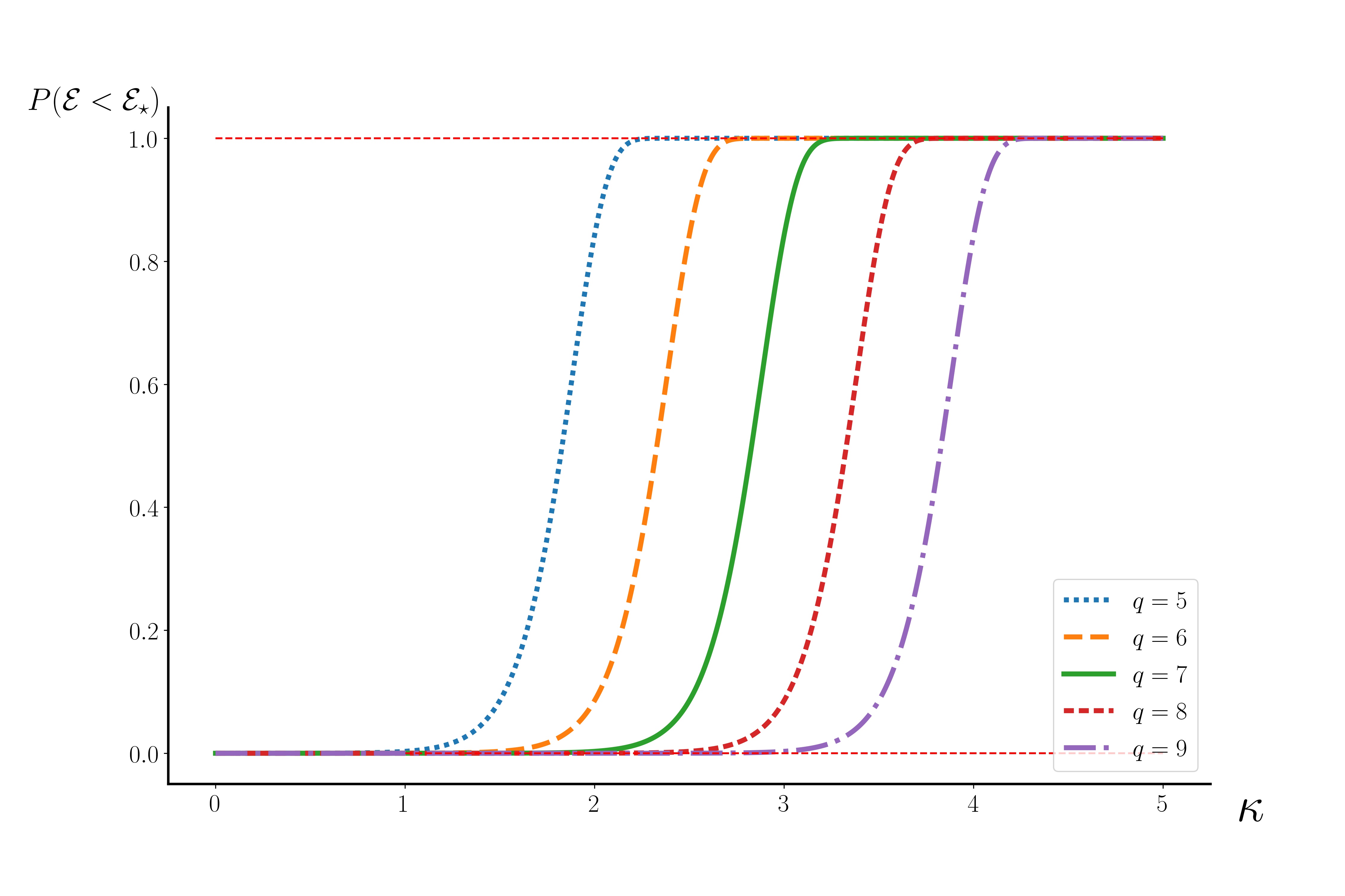
(97) As we concluded before, for , the observational constraint is satisfied for . However, equipped with the density function Eq. (92), it is better to study this issue using the language of the probability theory. The probability of having can be identified with the probability of where we have defined
(98) This probability is given by
(99) Here is the error function and , which in terms of our parameterization, is given by .
As shown in Fig 4, this probability depends on and on the initial conditions. For example if and , the probability that is less than is if the electric field is in its equilibrium state before the CMB scale modes leave the horizon. The important lesson is that the probabilistic interpretation, arising from the effects of the stochastic noises, allows us to relax significantly the observational upper bound on (or ) as compared to the bound obtained classically in Eq. (33). In conclusion, the anisotropic inflation model can be consistent with observations if we start with an electric field energy density larger than the classical attractor value, corresponding to .
4 Stochastic Dynamics of Scalar Field
To complete our studies of the stochastic effects on the system, here we present the Langevin equation associated with the inflaton field given by the Klein-Gordon equation (4).
Following the standard method [16, 17, 18], we split the inflaton field and its conjugate momentum into the long and short modes as follows,
| (100) | |||||
| (101) |
where, as before, the UV modes are defined in Fourier space as
| (102) | |||||
| (103) |
The next step is to expand the Klein-Gordon equation (4) around and up to first order in . Neglecting the magnetic field and using Eq. (13), we rewrite the last two terms of Eq. (4) as
| (104) | |||||
| (105) |
Therefore, for long wavelength mode we obtain
| (106) | |||
| (107) |
in which the noises are defined via
| (108) | |||||
| (109) |
As usual, the operator can be expanded in terms of the creation and annihilation operators, , in which is the positive frequency mode function satisfying the following equation
| (110) |
where we have used and . Furthermore, is the average effective mass of the long wavelength perturbations of the inflaton. We see that the inflaton’s effective mass receives corrections from the electric field which is the main reason for the system to attain its classical attractor solution in the mechanism of [3].
In order to solve Eqs. (106) and (107), we have to investigate the correlations of the noises and . Starting with the Bunch-Davies (Minkowski) vacuum , we obtain [18, 16]
| (111) | |||
| (112) | |||
| (113) |
with the following commutation relations
| (114) | |||||
| (115) |
From Eqs. (111)-(115), we find that for the parameter in the range [18, 16]
| (116) |
not only the quantum nature of and becomes negligible but also the -dependence disappears from (111)-(113). Furthermore, we obtain
| (117) | |||||
| (118) |
Hence Eqs. (106) and (107) reduce to a set of coupled classical Langevin equations,
| (119) | |||||
| (120) |
Considering the long wavelength modes where and working in the slow-roll limit where , the above two equations can be combined to yield the following Langevin equation for
| (121) |
in which is the normalized white classical noise related to via
| (122) |
satisfying
| (123) |
In the classical attractor regime , and one recovers the known classical equation [3]
| (124) |
By defining the dimensionless field , Eq. (121) is cast into
| (125) |
in which is the slow-roll parameter defined via . Taking the expectation value of the above equation yields the average of the scalar field velocity,
| (126) |
In the absence of stochastic effects and for the classical attractor regime (), the velocity is slowed down by the factor [3]. Now switching on the stochastic effects the velocity can be time-dependent based on the behaviour of , see Eqs. (80) and (86). In the case with where there is no stationary electric field probability distribution function, this may spoil inflation. However, in the equilibrium state with and , we can obtain a terminal velocity and the system reaches to an attractor regime. The terminal velocity can be obtained from (94) as
| (127) |
In Fig. 5, the dependency of the scalar field terminal velocity to the initial electric field energy density (controlled by the parameter ) is shown.

Below we estimate the mean value of the scalar field. Assuming (which is a consistent approximation in the slow-roll limit) we obtain
| (128) |
Here the integrand has different behaviour according to the initial values of the electric field:
- •
- •
:
This corresponds to the case in which the initial electric field amplitude is equal to the classical attractor initial condition () and the system evolves as a Wiener process with no drift. Substituting Eq. (86) into Eq. (128) we obtain(130) We see that the dependency of to the initial value of the electric field has disappeared when the system evolves as a Wiener process with no drift.
- •
:
Assuming that and the system is in its equilibrium state of electric field distribution, the expectation value of the scalar field is given by(131) where Eq. (94) has been used.
5 Summary and Discussions
In this work we have revisited the stochastic effects in the model of anisotropic inflation and derived the associated Langevin equations for the gauge field and inflaton field perturbations.
We have found that the fate of the electric field energy density in the presence of stochastic noises depends to some extend on the initial conditions. We have introduced the parameters and in which the former is a measure of the level of anisotropy (related to the initial parameter ) while the latter is a measure of the initial electric field energy density. In the region , corresponding to , the electric field components evolve more or less like a Brownian motion. Specifically, the variance of the electric field energy density increases linearly with the number of e-fold . As a result, the near isotropy condition is spoiled only after a large number of e-fold has elapsed, . The situation is more interesting when , corresponding to . Despite the fact that for the stochastic effects can not be ignored in one number of e-fold, but in all regions of the stochastic force is balanced by the classical force. Consequently, the probability density of electric field reaches a stationary state and the velocity of the scalar field approaches a terminal velocity. Hence, we suggest that the classical attractor mechanism of [3] with the electric field Eq. (19) is replaced by its stationary value Eq. (94). The mean-reversion phenomenon of Ornstein-Uhlenbeck process drives the system to the equilibrium state. This is similar to the classical feedback mechanism driving the system to its classical attractor regime, but considerably faster. The violation of isotropy condition yields which can not be met for realistic range of parameter , say . As a result, when , the predictions of the inflationary model can be consistent with cosmological observations if the system is in equilibrium regime by the time and the background electric field energy is given by its equilibrium value. This is one important difference of our analysis compared to the results of [13].
Another non-trivial result, as shown in Fig. 2, is that for the system falls into its stationary state much faster than the time required for the classical system to reach to its attractor regime. In the spacial case , the stochastic noises spoil the isotropy condition just when the system reaches to its classical attractor phase [3]. Finally, for , the electric field energy density grows continuously and the system does not reach to an equilibrium stage. As shown in Fig. 3, the number of e-folds when the near isotropy condition is violated is larger than the corresponding number of e-folds in classical system in the absence of noises.
Our findings partially disagree with those of [13] who have found that the probability for the statistical anisotropy to be consistent with the observational bounds is around . In addition, they concluded that this result is independent of the parameter and the initial value of the electric field. In the contrary, we have shown here that this probability is not small if the initial value of the electric field is larger than the classical attractor one . The details of this probability depends on the space of the parameters and can approach to .
Finally, we also have obtained the Langevin equation associated with the scalar field and have calculated the expectation values of the field and its velocity. We have shown that in the equilibrium state the velocity of the scalar field approaches to a terminal velocity which depends on the initial value of the electric field. The existence of a constant terminal velocity for the scalar field in the slow-roll regime reflects the fact that the scalar field falls into its attractor regime when the electric field is in its equilibrium state.
Acknowledgments: A. T. would like to thank Saramadan (Iran Science Elites Federation) for support.
Appendix A Noise Terms Correlation Functions
The correlation of electric field noises is given by
| (132) | |||||
where and we have used Eq. (27). At a fixed spatial point , the correlation is simplified to
| (133) |
Using Eq. (43), the correlation function at large-scale, , is given by
| (134) |
which can be rewritten as Eq. (58). Also the correlation of the momentum noises at a fixed spatial point can be calculated in the same way,
| (135) |
where . Hence on super-horizon scales, the correlation of the momentum noise is given by
| (136) |
where (43) is used. From this result we see that on large scales .
Appendix B Probability Distribution Function
Suppose we are given a random variable with probability distribution function (PDF) and accumulative distribution function which is defined as follows
| (137) |
Now let be the PDF and be the accumulative distribution function of , where is a real function. We then have
| (138) |
Calculating the PDF of needs the knowledge about the general behavior of and determining the domain of in which . We restrict ourselves to the case used in the paper. In other words we set . Hence we have
| (139) |
From the definition of the accumulative distribution function one can easily see that . Therefore for (139) we have
| (140) |
This is the expression we have used to determine the PDF of from , as discussed in the main draft.
The next important expression is the PDF of the sum of two random variables. Suppose and are two random variables. We would like to determine the PDF of . Suppose be the accumulative distribution and be the PDF of . Then we have
| (141) |
On the other hand, we can write
| (142) |
where is the conditional probability of if . Furthermore, one can write
| (143) |
So from Eqs. (142) and (143) one can deduce that
| (144) |
By taking the derivative of (144) we get the following equation for PDF of which is the convolution of and :
| (145) |
Now suppose we are given two independent random variables and whose PDF is given by Eq. (140). Note that and are two positive variables and so . Therefore we can write Eq. (144) for as
| (146) |
By repeating the above process one can obtain the PDF for sum of any arbitrary number of random variables. For three random variables we have
| (147) |
This is our starting point to derive the PDF of .
References
- [1] Y. Akrami et al. [Planck Collaboration], arXiv:1807.06211 [astro-ph.CO].
- [2] P. A. R. Ade et al. [Planck Collaboration], Astron. Astrophys. 594, A20 (2016), [arXiv:1502.02114 [astro-ph.CO]].
- [3] M. a. Watanabe, S. Kanno and J. Soda, Phys. Rev. Lett. 102, 191302 (2009).
- [4] P. A. R. Ade et al. [Planck Collaboration], Astron. Astrophys. 594, A16 (2016), [arXiv:1506.07135 [astro-ph.CO]].
- [5] J. Kim and E. Komatsu, Phys. Rev. D 88, 101301 (2013).
- [6] R. Emami, arXiv:1511.01683 [astro-ph.CO].
- [7] M. a. Watanabe, S. Kanno and J. Soda, Prog. Theor. Phys. 123, 1041 (2010).
- [8] N. Bartolo, S. Matarrese, M. Peloso and A. Ricciardone, Phys. Rev. D 87, no. 2, 023504 (2013).
- [9] R. Emami and H. Firouzjahi, JCAP 1310, 041 (2013)
- [10] A. A. Abolhasani, R. Emami, J. T. Firouzjaee and H. Firouzjahi, JCAP 1308, 016 (2013).
- [11] A. Naruko, E. Komatsu and M. Yamaguchi, JCAP 1504, no. 04, 045 (2015).
- [12]
S. Kanno, J. Soda, M. -a. Watanabe,
JCAP 1012, 024 (2010).
J. Ohashi, J. Soda and S. Tsujikawa,
JCAP 1312, 009 (2013).
J. Ohashi, J. Soda and S. Tsujikawa,
Phys. Rev. D 88, 103517 (2013).
J. Ohashi, J. Soda and S. Tsujikawa,
Phys. Rev. D 87, 083520 (2013).
S. Yokoyama and J. Soda,
JCAP 0808, 005 (2008).
A. Ito and J. Soda,
Phys. Rev. D 92, no. 12, 123533 (2015).
A. Ito and J. Soda,
JCAP 1604, no. 04, 035 (2016).
A. Ito and J. Soda,
Eur. Phys. J. C 78, no. 1, 55 (2018).
K. Murata, J. Soda,
JCAP 1106, 037 (2011).
K. Yamamoto, M. -a. Watanabe and J. Soda,
Class. Quant. Grav. 29, 145008 (2012).
A. E. Gumrukcuoglu, B. Himmetoglu, and M. Peloso,
Phys. Rev. D 81, 063528 (2010)
[arXiv:1001.4088 [astro-ph]].
R. Emami, H. Firouzjahi, S. M. Sadegh Movahed and M. Zarei,
JCAP 1102, 005 (2011)
R. Emami and H. Firouzjahi,
JCAP 1201, 022 (2012)
A. A. Abolhasani, R. Emami and H. Firouzjahi,
JCAP 1405, 016 (2014)
S. Baghram, M. H. Namjoo and H. Firouzjahi,
JCAP 1308, 048 (2013).
A. A. Abolhasani, R. Emami and H. Firouzjahi,
JCAP 1405, 016 (2014).
R. Emami, H. Firouzjahi and M. Zarei,
Phys. Rev. D 90, no. 2, 023504 (2014).
A. A. Abolhasani, M. Akhshik, R. Emami and H. Firouzjahi,
JCAP 1603, 020 (2016).
X. Chen, R. Emami, H. Firouzjahi and Y. Wang,
JCAP 1408, 027 (2014).
T. Rostami, A. Karami and H. Firouzjahi,
JCAP 1706, no. 06, 039 (2017).
T. R. Dulaney and M. I. Gresham,
Phys. Rev. D 81, 103532 (2010),
M. Shiraishi, E. Komatsu, M. Peloso and N. Barnaby,
JCAP 1305, 002 (2013).
M. Shiraishi, E. Komatsu and M. Peloso,
JCAP 1404, 027 (2014).
N. Barnaby, R. Namba and M. Peloso,
Phys. Rev. D 85, 123523 (2012).
K. Dimopoulos, M. Karciauskas, D. H. Lyth and Y. Rodriguez,
JCAP 0905, 013 (2009).
T. Fujita and S. Yokoyama,
JCAP 1309, 009 (2013).
S. R. Ramazanov and G. Rubtsov,
Phys. Rev. D 89, 043517 (2014).
S. Nurmi and M. S. Sloth,
JCAP 1407, 012 (2014).
R. K. Jain and M. S. Sloth,
JCAP 1302, 003 (2013).
F. R. Urban,
Phys. Rev. D 88, 063525 (2013).
M. Thorsrud, D. F. Mota and S. Hervik,
JHEP 1210, 066 (2012).
S. Bhowmick and S. Mukherji,
Mod. Phys. Lett. A 27, 1250009 (2012).
S. Hervik, D. F. Mota and M. Thorsrud,
JHEP 1111, 146 (2011).
C. G. Boehmer, D. F. Mota,
Phys. Lett. B663, 168-171 (2008).
T. S. Koivisto, D. F. Mota,
JCAP 0808, 021 (2008).
D. H. Lyth and M. Karciauskas,
JCAP 1305, 011 (2013).
Tuan Q. Do and W. F. Kao,
Phys. Rev. D 84, 123009.
Tuan Q. Do, W. F. Kao, and Ing-Chen Lin, Phys. Rev. D 83, 123002. T. Fujita, I. Obata, T. Tanaka and S. Yokoyama, JCAP 1807, 023 (2018). A. Talebian-Ashkezari, N. Ahmadi and A. A. Abolhasani, JCAP 1803, no. 03, 001 (2018). A. Talebian-Ashkezari and N. Ahmadi, JCAP 1805, no. 05, 047 (2018). K. Choi, K. Y. Choi, H. Kim and C. S. Shin, JCAP 1510, no. 10, 046 (2015). J. Holland, S. Kanno and I. Zavala. arXiv:1711.07450 [hep-th]. K. Yamamoto, Phys. Rev. D 85, 123504 (2012). H. Funakoshi and K. Yamamoto, Class. Quant. Grav. 30, 135002 (2013). R. Emami, S. Mukohyama, R. Namba and Y. l. Zhang, JCAP 1703, no. 03, 058 (2017). V. Papadopoulos, M. Zarei, H. Firouzjahi and S. Mukohyama, Phys. Rev. D 97, no. 6, 063521 (2018). - [13] T. Fujita and I. Obata, JCAP 1801, no. 01, 049 (2018), [arXiv:1711.11539 [astro-ph.CO]].
- [14] A. A. Starobinsky, Lect. Notes Phys. 246, 107 (1986).
- [15] A. D. Linde, Phys. Lett. B 175, 395 (1986).
- [16] M. Sasaki, Y. Nambu and K. i. Nakao, Nucl. Phys. B 308, 868 (1988).
- [17] Y. Nambu and M. Sasaki, Phys. Lett. B 219, 240 (1989).
- [18] K. i. Nakao, Y. Nambu and M. Sasaki, Prog. Theor. Phys. 80, 1041 (1988).
- [19] S. Mollerach, S. Matarrese, A. Ortolan and F. Lucchin, Phys. Rev. D 44, 1670 (1991).
- [20] A. A. Starobinsky and J. Yokoyama, Phys. Rev. D 50, 6357 (1994).
- [21] F. Finelli, G. Marozzi, A. A. Starobinsky, G. P. Vacca and G. Venturi, Phys. Rev. D 79, 044007 (2009).
- [22] F. Finelli, G. Marozzi, A. A. Starobinsky, G. P. Vacca and G. Venturi, Phys. Rev. D 82, 064020 (2010).
- [23] K. Enqvist, D. G. Figueroa and G. Rigopoulos, JCAP 1201, 053 (2012).
- [24] J. Martin and V. Vennin, Phys. Rev. D 85, 043525 (2012).
- [25] M. Kawasaki and T. Takesako, JCAP 1208, 031 (2012).
- [26] T. Fujita, M. Kawasaki, Y. Tada and T. Takesako, JCAP 1312, 036 (2013).
- [27] T. Fujita, M. Kawasaki and Y. Tada, JCAP 1410, no. 10, 030 (2014).
- [28] V. Vennin and A. A. Starobinsky, Eur. Phys. J. C 75, 413 (2015).
- [29] J. Tokuda and T. Tanaka. arXiv:1708.01734 [gr-qc].
- [30] A. Vilenkin, Nucl. Phys. B 226, 527 (1983).
- [31] Y. Nambu and M. Sasaki, Phys.Lett. B205 (1988) 441.
- [32] H. E. Kandrup, Phys.Rev. D39 (1989) 2245.
- [33] Y. Nambu, Prog.Theor.Phys. 81 (1989) 1037.
- [34] A. D. Linde, D. A. Linde, and A. Mezhlumian, Phys.Rev. D49 (1994) 1783–1826.
- [35] K. E. Kunze, JCAP 0607, 014 (2006).
- [36] T. Prokopec, N. C. Tsamis and R. P. Woodard, Annals Phys. 323, 1324 (2008).
- [37] T. Prokopec, N. C. Tsamis and R. P. Woodard, Phys. Rev. D 78, 043523 (2008).
- [38] N. C. Tsamis and R. P. Woodard, Nucl. Phys. B 724, 295 (2005).
- [39] K. Enqvist, S. Nurmi, D. Podolsky and G. I. Rigopoulos, JCAP 0804, 025 (2008).
- [40] B. Garbrecht, G. Rigopoulos, and Y. Zhu, Phys.Rev. D89 (2014) 063506.
- [41] B. Garbrecht, F. Gautier, G. Rigopoulos, and Y. Zhu, Phys. Rev. D91 (2015), no. 6 063520.
- [42] C. P. Burgess, R. Holman, G. Tasinato and M. Williams, JHEP 1503, 090 (2015).
- [43] C. P. Burgess, R. Holman and G. Tasinato, JHEP 1601, 153 (2016).
- [44] D. Boyanovsky, Phys. Rev. D 92, no. 2, 023527 (2015).
- [45] D. Boyanovsky, Phys. Rev. D 93, 043501 (2016).
- [46] V. Vennin, H. Assadullahi, H. Firouzjahi, M. Noorbala and D. Wands, Phys. Rev. Lett. 118, no. 3, 031301 (2017).
- [47] H. Assadullahi, H. Firouzjahi, M. Noorbala, V. Vennin and D. Wands, JCAP 1606, no. 06, 043 (2016).
- [48] J. Grain and V. Vennin, JCAP 1705, no. 05, 045 (2017).
- [49] M. Noorbala, V. Vennin, H. Assadullahi, H. Firouzjahi and D. Wands, JCAP 1809, no. 09, 032 (2018).
- [50] H. Firouzjahi, A. Nassiri-Rad and M. Noorbala, JCAP 1901, no. 01, 040 (2019).
- [51] L. Evans, “An introduction to stochastic differential equations,” American Mathematical Society (2013).