On a convergence property of a geometrical algorithm for statistical manifoldsThanks: This is a full version of the paper presented in ICONIP2019
Abstract
In this paper, we examine a geometrical projection algorithm for statistical inference. The algorithm is based on Pythagorean relation and it is derivative-free as well as representation-free that is useful in nonparametric cases. We derive a bound of learning rate to guarantee local convergence. In special cases of m-mixture and e-mixture estimation problems, we calculate specific forms of the bound that can be used easily in practice.
1 Introduction
Information geometry is a framework to analyze statistical inference and machine learning[2]. Geometrically, statistical inference and many machine learning algorithms can be regarded as procedures to find a projection to a model subspace from a given data point. In this paper, we focus on an algorithm to find the projection.
Since the projection is given by minimizing a divergence, a common approach to finding the projection is a gradient-based method[6]. However, such an approach is not applicable in some cases. For instance, several attempts to extend the information geometrical framework to nonparametric cases[3, 9, 13, 15], where we need to consider a function space or each data is represented as a point process. In such a case, it is difficult to compute the derivative of divergence that is necessary for gradient-based methods, and in some cases, it is difficult to deal with the coordinate explicitly.
Takano et al.[15] proposed a geometrical algorithm to find the projection for nonparametric e-mixture distribution, where the model subspace is spanned by several empirical distributions. The algorithm that is derived based on the generalized Pythagorean theorem only depends on the values of divergences. It is derivative-free as well as representation-free, and it can be applicable to many machine learning algorithms that can be regarded as finding a projection, but its convergence property has not been analyzed yet. The first contribution of this paper is to extend the algorithm to more general cases. The second contribution is to give a condition for the convergence of the algorithm, which is given as a bound of learning rate. In the case of the discrete distribution, we obtain specific forms of the bound that can be used easily in practice.
2 Geometrical algorithm
2.1 Projection in a statistical manifold
Here we briefly review the information geometry in order to explain the proposed geometrical algorithm based on generalized Pythagorean theorem[12].
Let be a statistical manifold, where is a smooth manifold with a Riemannian metric , dual affine connections and . We consider the case that is (dually) flat, where there exist a -affine coordinate and a -affine coordinate . For a flat manifold, there exist potential functions and , and the two coordinates and are transformed each other by Legendre transform,
| (1) |
A typical example of a flat manifold is an exponential family, where each member of the manifold is a distribution of a random variable with parameter ,
| (2) |
where is a sufficient statistics and is a normalization factor. For the exponential family, there are two dual connections, called e-connection and m-connection (e: exponential, m: mixture). If we take the e-connection as the -connection, -affine coordinate is equal to called e-coordinate, and -affine coordinate called m-coordinate is given by
| (3) |
where the function becomes a potential function . Note that if we take the m-connection as , the relation changes in a dual way, i.e., becomes and becomes .
Here, for , we denote the corresponding - and -coordinate by and respectively. Let us consider a submanifold defined by linear combination of points ,
| (4) |
where is a weight vector whose sum is 1. The submanifold is an affine subspace and hence it is called an -autoparallel (or -flat) submanifold. In particular, if , is a straight line of -coordinate that is called -geodesic.
We can also consider another submanifold in the dual coordinate,
| (5) |
which is called a -autoparallel (or -flat) submanifold. The -geodesic is defined by a straight line of -coordinate.
Now let us define a -projection and a -projection from a point onto a submanifold . The -projection is a point such that -geodesic between and is orthogonal to at with respect to the Riemannian metric . In the statistical manifold, is taken as
| (6) |
which is equal to Fisher information for exponential family
| (7) |
In a similar way, -projection onto a submanifold is defined as a point so that the -geodesic connecting and is orthogonal to .
Theorem 1 (Generalized Pythagorean theorem[12]).
Let be a -autoparallel submanifold of a statistical manifold , and the -projection be from a point , then for any point , the following relation holds
| (8) |
where is the canonical divergence defined by
| (9) |
By exchanging and , we have a dual relation, i.e, for a -autoparallel submanifold , the -projection from a point satisfies the relation
| (10) |
where and is a dual divergence defined by .
From this theorem, we see that a -projection (-projection) onto a -autoparallel (-autoparallel respectively) submanifold is unique and can be found by minimizing corresponding divergence, i.e., the -projection is given by
| (11) |
and the -projection is given by
| (12) |
For the exponential family (2), taking the e-connection as -connection, the divergence is equal to the Kullback-Leibler divergence,
| (13) |
If we take the e-connection as or connection, the corresponding projection and autoparallel submanifold is called an e-projection and an e-autoparallel submanifold, and similarly, an m-projection and an m-autoparallel submanifold are defined for the m-connection.
2.2 Geometrical algorithm for projection
Now we propose a geometrical algorithm to find a -projection (or -projection) onto a -autoparallel (and -autoparallel respectively) submanifold. To avoid redundant description, we only formulate the -projection onto a -autoparallel submanifold, since the dual case can be obtained by only exchanging and .
In this paper, we impose a restriction on the projection.
Although the projection from a point does not necessarily belong to the convex hull of basis vectors in general, some application such as mixture models that will be explained in Sec. 4.1 requires this assumption. We will discuss this restriction in Sec. 6.3.

Suppose a point and a -autoparallel submanifold are given, let be a current estimate of the projection (Fig. 1) and let us define the quantity ,
| (14) |
From Eq. (8), if and only if . If , that means is closer to than , should be decreased. On the other hand, if , is farther from than , should be increased.
From the consideration above, we can construct the Algorithm 1 to find the -projection by optimizing weights so that satisfies the Pythagorean relation (8).
| (15) |
| (16) |
In the algorithm, the function is a positive and strictly monotonically increasing function s.t. , which is introduced in order to stabilize the algorithm and a typical choice of is a sigmoidal function,
| (17) |
A parameter controls the learning speed and it is related to convergence characteristics of the algorithm. Algorithm A() in the case that m-connection is taken as -connection was firstly introduced by Takano et al.[15] in order to estimate a nonparametric e-mixture distribution. The main contribution of this paper is to clarify the relation between the function and the convergence property. In later sections, we prove Algorithm A() (and also Algorithm A()) is locally stable if the derivative of at the origin is less than a certain bound. For later theoretical analysis, we show the following Lemma here.
Lemma 3.
The value in Algorithm A() is given by
| (18) |
which means that only depends on the points on , if the true projection is known.
Proof.
For any and , let us define
| (19) |
The value is given by
| (20) |
From the Pythagorean theorem,
| (21) |
thus becomes (18). ∎
3 Stability analysis in the case of
We start the analysis from the simplest case of . As shown later, the case of general is reduced to this case. From (18), is only depends on the points on the , and if , is just a one-dimensional straight line of .
3.1 Behavior of
In order to derive the condition for convergence, we examine the behavior of for a small perturbation.
The weight value can be regarded as an -coordinate of , and let be the -coordinate that is dual to . Let be the value of at the projection point , and the current estimation is perturbed slightly from ,
| (22) |
then from (18), the value is given by
| (23) |
where and are the value at and respectively, and
| (24) |
When is small, it can be expanded upto the first order of ,
| (25) |
where
| (26) |
is Jacobian that is equal to Riemannian metric
| (27) |
and is also obtained by
| (28) |
As a result, we have
| (29) |
Similarly,
| (30) |
3.2 The condition for local stability of the Algorithm A()
In this section, we show the condition for local convergence property of the Algorithm A(). Here we call the algorithm is locally stable when the amount of sufficiently small perturbation from the optimal solution is decreased by the algorithm.
Theorem 4.
Algorithm A() is locally stable when it holds
| (31) |
where is the optimal weight.
Proof.
By the Algorithm A(), the weight is updated by
| (32) |
and its first order expansion is given from Eq. (29) by
| (33) |
and for ,
| (34) |
We see that , thus the normalization procedure is negligible up to the first order of .
The condition that is a stable point of the algorithm is given by
| (35) |
From Eq. (33), it is
| (36) |
which is equivalent to
| (37) |
then we have
| (38) |
∎
Since the true value is not known when the algorithm is applied, we have two approaches. The one is approximating by the current estimate and use adaptively changing the derivative of , which will be examined in sec.6.2. The other approach is to use a bound that is independent of , which is available in some special cases.
Corollary 5.
Algorithm A() is locally stable when it holds
| (39) |
where we denote for simplicity.
4 Special case: discrete distribution
In the following subsections, we give specific forms of the bound of Eq. (39) both for the e-projection and m-projection by considering a discrete distribution as a specific case.
The discrete distribution is given by
| (40) |
| (41) |
where when and otherwise. We see that the discrete distribution belongs to the exponential family as follows:
| (42) |
where we have independent parameters and one dependent parameter is given by . By taking the e-connection as the -connection, becomes the same form as Eq. (2) by regarding
| (43) |
The dual coordinate is given by
| (44) |
The basis vectors in are denoted by
| (45) |
4.1 The case of e-projection
First, we take the e-connection as the -connection, then the -projection onto the -autoparallel submanifold is the e-projection onto the m-autoparallel submanifold.
The m-autoparallel submanifold spanned by is given by a set of points whose m-coordinate (44) is given by
| (46) |
Since is the probability value, it is equivalent to the mixture distribution of
| (47) |
where is usually assumed to be positive, which matches the Assumption 2.
The mixture distribution has a lot of applications, in which complicated distribution is decomposed into sum of simple component distributions. An important application in the discrete distribution case is the nonnegative matrix factorization[10], where a matrix with nonnegative components is approximated by
| (48) |
where and are also matrices with nonnegative components. Let be the normalization operator by which sum of each column components become 1. It is known[5] that if , there exist and such that
| (49) |
where and are matrices with nonnegative components and sum of each column components is 1. This means that a set of probability distributions are approximated by mixture of factor distributions. In the NMF, and are optimized alternatively by fixing the other. Each optimization problem can be regarded as e-projection to m-autoparallel manifold.
Note that we consider the e-projection onto an m-autoparallel submanifold in this paper, since it is natural from the generalized Pythagorean relation. However, many learning algorithms are formulated to maximum likelihood that is equivalent to the m-projection, which is different from e-projection in the sense that the argument of divergence is reversed. For the discrete distribution case, the m-projection to the m-autoparallel submanifold has a unique solution, but it does not hold in general.
Now we give a sufficient condition for convergence of the e-projection onto the m-autoparallel submanifold.
Proposition 6.
The Algorithm A() of the e-projection onto an m-autoparallel submanifold for the discrete distribution locally stable if
| (50) |
where the right hand side has a constant lower bound .
Proof.
The m-autoparallel model spanned by points can be written as
| (51) |
The Riemannian metric at is given by
| (52) |
The denominator of right hand side of Eq. (39) is
| (53) |
The -th term
| (54) |
has maximum value when , then Eq. (53) is bounded from upper by
| (55) |
which is a Hellinger distance between and , and we obtain the sufficient condition for local stability,
| (56) |
and the right hand side has a constant lower bound . ∎
4.2 The case of m-projection
In this subsection, we take the m-connection as the -connection, then the -projection onto the -autoparallel submanifold is the m-projection onto the e-autoparallel submanifold.
The e-autoparallel submanifold spanned by is given by a set of points whose e-coordinate (43) is given by
| (57) |
Since , it is equivalent to the model specified by
| (58) |
which is a different type of mixture, log linear mixture.
We call this type of mixture as e-mixture, while the mixture specified by Eq. (47) as m-mixture. Although the e-mixture has not been studied as intensively as the m-mixture, it has several good properties such as maximum entropy principle. Takano et al.[15] proposed a nonparametric extension of the e-mixture and its learning algorithm based on the geometrical algorithm, which is generalized in this paper. In the nonparametric e-mixture estimation, the basis distributions are expressed by the empirical distribution (i.e., sum of delta functions), thus the e-mixture of basis distibutions cannot mathematically defined. Instead, it is defined by geometrical characteristics of e-mixture[11]. Therefore, it is not possible to obtain the coordinate explicitly. Because the geometrical algorithm is coordinate-free, and it only requires to calculate divergences, which can be estimated based on nonparametric entropy estimation[8, 7]. This is a strong motivation to propose the geometrical algorithm.
Here we give a sufficient condition for convergence of the m-projection onto the e-autoparallel submanifold.
Proposition 7.
The Algorithm A() of the m-projection onto the e-autoparallel submanifold for the discrete distribution is locally stable if
| (59) |
The right hand side does not have a constant lower bound unlike the e-projection case, and it is left as an open problem whether there exists any constant bound.
Proof.
The e-autoparallel model for is written as
| (60) |
where is an e-coordinate, is a normalization constant
| (61) |
Since the discrete distribution
| (62) |
is written as
| (63) |
where
| (64) |
| (65) |
Note that
The Fisher information for this model can be calculated by
| (66) |
The last formula represents the variance of with respect to the probability weight . From Popoviciu’s inequality on variances[14], has an upper bound that is independent of ,
| (67) |
Since , we obtain the inequality (59) of the Proposition from Eq. (39). ∎
5 Local stability for general
We proceed to the general case which include . First we present the main theorem.
Theorem 8.
Let , be the optimal parameter. If the function satisfies
| (68) |
Algorithm A() is locally stable.
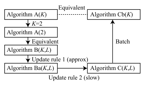
The proof is in the appendix. Basic strategy of the proof is to show the equivalence between the Algorithm A() and a component-wise update algorithm based on Algorithm A(). In the process of the proof, a possible refinement of the Algorithm A() is also suggested.
6 Discussion
In this section, we will discuss several points related to the proposed framework, (1) relation to gradient descent method, (2) possible refinement of the algorithm, (3) assumption of the positivity.
6.1 Relation to gradient descent method
In general optimization problems, a gradient descent method is a simple way to solve the problem. Here, we show that the updates of the gradient descent and the proposed algorithm are linearly related.
The parameter should satisfy a constraint . We first replace by , then update for by
| (69) |
and is obtained by .
The gradient of with respect to is given by
| (70) |
Since
| (71) |
and , we have
| (72) |
which can be, from Lemma 3, represented using ,
| (73) |
The amount of update by the gradient descent is
| (74) |
and
| (75) |
On the other hand, the amount of update by the Algorithm A() is approximated for small by
| (76) |
Since , no further normalization is necessary. Comparing Eq. (74) and Eq. (75) with Eq. (76), we see that and are linearly related. Unlike the gradient descent method, the proposed framework does not need explicit calculation of the coodinate.
6.2 Possible refinement of the algorithm
As explained in Sec. 3.2, the condition for convergence depends on the true parameter, thus one approach to use the adaptively change the derivative of is to replace the true parameter by its estimate. This approach also requires to estimate the Fisher information.
Another possibility for the refinement of the algorithm is based on the analysis in the appendix. It will be shown that the Algorithm A() is equivalent to the slower version of the component-wise update algorithm. More specifically, the amount of the update is smaller by the factor . Therefore, the update rule in the Algorithm A(), can be replaced by
| (77) |
which does not change the condition of the convergence.
6.3 On the assumption of positivity
In Sec. 2.2, we assumed that the projection lies on the convex hull spanned by the basis vectors. In general, however, the projection point can be out of . In such a case, we generalize the problem to find a point on that minimizes the divergence,
| (78) |
When the projection point is out of , the solution of this problem is on the boundary of and the -geodesic connecting and is not orthogonal to any more.
The proposed algorithm itself works even in this case, because the boundary is again a convex hull of a subset of basis vectors. However, we have to be careful about one thing: once a certain becomes 0, it cannot take positive value any longer, which means that if the current estimate reaches to the boundary that does not include the optimal solution, then the estimator cannot escape from the boundary.
Without the assumption of , the -projection of to a dual autoparallel submanifold always exists uniquely and such a formulation is studied as e-PCA and m-PCA framework[1] or exponential family PCA in a special case[4]. However, the algorithm proposed in this paper cannot be applied as it is, because it is derived under the assumption. One method of update for this general case is as follows: should be increased for positive and should be decreased for negative . Also, should be preserved. Therefore, let be a set of indices with positive and be a set of indices with negative . Then
| (79) |
for a learning constant . There are several variations of such an update, and we also have to take care the update does not make out of the domain of . The investigation of convergence property of the modified algorithm is left as a future work.
7 Concluding remarks
We proposed a geometrical projection algorithm that only requires the calculation of divergences. We also showed the condition of the local stability of the algorithm. There are various applications in machine learning and related areas in which the projection onto an autoparallel submanifold is needed, and they are left as future works.
Acknowledgement
This work was supported by JSPS KAKENHI Grant Numbers 17H01793, 19K12111.
References
- [1] Shotaro Akaho. The e-PCA and m-PCA: Dimension reduction of parameters by information geometry. In Neural Networks, 2004. Proceedings. 2004 IEEE International Joint Conference on, volume 1, pages 129–134. IEEE, 2004.
- [2] Shunichi Amari. Information geometry and its applications, volume 194. Springer, 2016.
- [3] Nihat Ay, Jürgen Jost, Hông Vân Lê, and Lorenz Schwachhöfer. Information geometry, volume 64. Springer, 2017.
- [4] Michael Collins, Sanjoy Dasgupta, and Robert E Schapire. A generalization of principal component analysis to the exponential family. In NIPS, volume 13, page 23, 2001.
- [5] Bo Dong, Matthew M Lin, and Moody T Chu. Nonnegative rank factorization—a heuristic approach via rank reduction. Numerical Algorithms, 65(2):251–274, 2014.
- [6] Akio Fujiwara and Shunichi Amari. Gradient systems in view of information geometry. Physica D: Nonlinear Phenomena, 80(3):317–327, 1995.
- [7] Hideitsu Hino, Shotaro Akaho, and Noboru Murata. An Entropy Estimator Based on Polynomial Regression with Poisson Error Structure. In Neural Information Processing - 23rd International Conference, ICONIP 2016, Kyoto, Japan, October 16-21, 2016, Proceedings, Part II, pages 11–19, 2016.
- [8] Hideitsu Hino, Kensuke Koshijima, and Noboru Murata. Non-parametric entropy estimators based on simple linear regression. Computational Statistics & Data Analysis, 89(0):72 – 84, 2015.
- [9] Guy Lebanon et al. Riemannian geometry and statistical machine learning. LAP LAMBERT Academic Publishing, 2015.
- [10] Daniel D Lee and H Sebastian Seung. Learning the parts of objects by non-negative matrix factorization. Nature, 401(6755):788–791, 1999.
- [11] Noboru Murata and Yu Fujimoto. Bregman divergence and density integration. Journal of Math-for-Industry (JMI), 1(B):97–104, 2009.
- [12] Hiroshi Nagaoka and Shunichi Amari. Differential geometry of smooth families of probability distributions. Technical Report METR 82-7, University of Tokyo, 1982.
- [13] Giovanni Pistone. Nonparametric information geometry. In Geometric Science of Information, pages 5–36. Springer, 2013.
- [14] Tiberiu Popoviciu. Sur les équations algébriques ayant toutes leurs racines réelles. Mathematica (Cluj), 9:129–145, 1935.
- [15] Ken Takano, Hideitsu Hino, Shotaro Akaho, and Noboru Murata. Nonparametric e-mixture estimation. Neural Computation, 28(12):2687–2725, 2016.
Appendix Proof of Theorem 8
A.1 Component-wise algorithm
Suppose the point be the point where the extension line from through intersects with the boundary of (Fig. 3). Let us introduce the notation to specify the point of ,
| (80) |
for instance and . Since , and are on the same line, by taking an appropriate ,
| (81) |
or equivalently,
| (82) |
For the , should be zero,
| (83) |
that is
| (84) |
and the point is given by
| (85) |
We can consider the component-wise update for by using and .
More detailed procedures of (a) and (b) are described later. In the algorithm, the number controls how each component-wise update converges, which plays an important role for fast convergence as will be demonstrated in Sec. A.3.
Proposition 9.
If the condition of local stability for is satisfied for all , Algorithm B() is locally stable for any .
Now let us give the procedures in Algorithm B(). The algorithm between and , the current solution should be represented in the form of
| (86) |
where , and then calculate and based on the Pythagorean relation, and then apply the update (15) and (16). From Eq. (81),
| (87) |
then the weights for and are obtained as and respectively. The update of is written as
| (88) |
and then normalization is performed as
| (89) |
From Eqs. (85) and (86), we have
| (90) |
By updating and to and respectively, then the corresponding update of is given by
| (91) |
This update requires to calculate (and related values), which increases the computational complexity. For later discussions, let us rewrite the algorithm when the amount of update is sufficiently small. From the discussion on the analysis of (Eq.(3.2)), if the update is sufficiently small,
| (92) |
holds, where represents the neglecting higher order terms of . By this approximation, the update is simplified as follows:
Update rule 1:
| (93) |
Note that calculating is not necessary any longer. Based on the Update rule 1, the algorithm is simplified.
Algorithm Ba() behaves similarly to Algorithm B() locally and it requires smaller computation cost.
Proposition 10.
If the condition of local stability for is satisfied for all , Algorithm Ba() is locally stable for any .
A.2 One-side component-wise update
The component-wise update without any approximation requires to find , which may cause additional complexity compared to the Algorithm A(). Here we consider a simpler algorithm: only the -th weight is updated with fixing other weights and normalize all weights, that is,
Update rule 2:
| (94) |
This update does not require the computation of . We examine the relation between Update 1 and 2. Assuming is sufficiently small, the Update 2 is approximated by
| (95) |
| (96) |
which means that the Update rule 2 is equivalent to the Update rule 1 where the learning constant is shortened by a factor .
Therefore, we see that if the Update rule 1 is locally stable, the Update rule 2 is also locally stable.
In a similar way with component-wise algorithm, we can obtain one-side component-wise algorithm for general based on Update rule 2.
Note that updating affects the value of other () because of the normalization.
Proposition 11.
If the condition of local stability for is satisfied for all , Algorithm C() is locally stable for any .
A.3 Local stability of the Algorithm A()
Now we are ready to prove the local stability of Algorithm A().
The Algorithm C() is a sequential algorithm, and we can construct corresponding “batch” version of the algorithm.
Since Algorithm Cb() updates the weights by perturbations, the condition for local stability is changed. The following lemma gives a sufficient condition.
Lemma 12.
Algorithm Cb() is locally stable if satisfies
| (99) |
where denotes the optimal value.
This bound is given by multiplying to (39), but it might be very strict, because (39) for is a better bound. Further, as wee see, Algorithm Cb() is very similar to Algorithm C(), where only the difference is whether the former is a simultaneous update and the latter is a sequential update. It is an open problem to obtain a better bound for .
Proof.
By the update of , suppose the weight is changed from to , where because of the weight constraint. If satisfies the condition (39), it holds
| (100) |
for all . By multiplying to the value of , the change of weights becomes in terms of the first order approximation, and the simultaneous update of the all weight, it becomes . Therefore, the new weight satisfies
| (101) |
which shows local stability of Algorithm Cb(). ∎
The main theorem 8 is proved by showing equivalence between Algorithm A() and Algorithm Cb() as follows.
Lemma 13.
When the update amounts of are sufficiently small, The Algorithm A() is equivalent to Algorithm Cb().
Proof.
By the Algorithm A(), the weights are updated by
| (102) |
| (103) |
On the other hand, the update of in the Update rule 2 for small is given by (95) and (96). Therefore, the amount of change of for the update of is given by
| (104) |
then summing up them and we have the update of of the Algorithm Cb() by
| (105) |
which coincides the update of (103). ∎