Quantumness of Relative Incompatibility

It is generally believed that quantum superposition and entanglement are two primordial quantum features, which are responsible for giving us significant advantages in the field of secure communication and computation over the digitized information system Ekert 1991; Bennett and Brassard 2014; Shor and Preskill 2000; Adhikari et al. 2010; Bose et al. 1998. However, these are not exhaustive features that are akin to quantum systems. Lately, relevant concepts like quantum correlations beyond entanglement Ollivier and Zurek 2001; Henderson and Vedral 2001; Modi et al. 2010; Chakrabarty et al. 2011, coherence of quantum state Winter and Yang 2016, set of stronger uncertainty relations Maccone and Pati 2014; Song et al. 2017; Wang et al. 2016; Mukhopadhyay et al. 2016 and coherence of purification Pati et al. 2019 came into picture, where each of these concepts tell something about the quantum system. All these come under the umbrella of a universally accepted term called "quantumness". This motivates us to re-conceptualize the idea of what is quantum in a quantum state.

In particular, quantum coherence can be viewed as a fundamental signature of non-classicality in physical systems. It tries to capture the superposition or wave aspect of a single quantum system Winter and Yang 2016; Baumgratz et al. 2014; Aberg 2006. Coherence can also be used as a resource for certain tasks like better cooling Brask and Brunner 2015; Lostaglio et al. 2015 or work extraction processes in nano-scale thermodynamics, many quantum algorithms Anand and Pati 2016; Shi et al. 2017; Olaya-Castro et al. 2008, quantifying wave-particle duality Bera et al. 2015; Yuan et al. 2018; Abbott et al. 2008 and in biological processes Bandyopadhyay et al. 2012; Wilde et al. 2009. The resource theory of quantum coherence Streltsov et al. 2015; Asbóth et al. 2005; Xi et al. 2015; Streltsov et al. 2016; Qi et al. 2017; Chin 2017; Zhu et al. 2017; Zhu et al. 2018; Korzekwa et al. 2016 along with other resource theories of entanglement and thermodynamics Hillery 2016; Napoli et al. 2016, have also been established. Recently, a resource theory framework for the particle nature of a quantum system was introduced Das et al. 2018 which quantifies what we mean by a ’particle’ in quantum world.

Effort to understand and quantify the quantumness in a single pure quantum system is still not complete, and hence, it requires more investigation. Our idea is to quantify quantumness in a state as something that will depend on observables of our choice. Quantum coherence reveals one aspect of quantumness with respect to one observable (that fixes the basis). Here, in this article, we formalize the quantumness of the relative incompatibility of a state with respect to two non-commuting observables. Relative incompatibility is defined as relative entropy between the two marginal probability distribution of the outcomes of joint probability distributions. These joint probability distributions are obtained when measurements of the two non-commuting observables are performed in different order. We call this as the quantumness of relative incompatibility. We show that our measure satisfies standard properties like convexity and additivity. We also show that for a pure quantum state, the quantumness shows complementary behaviour with the coherence of a system when we measure the coherence in the eigen basis of one of the observables. This indicates that quantumness may be fundamentally different concept than quantum coherence.

This article is organized as follows: section II begins by defining quantumness of a state. We show that it satisfies several realisable properties which are required to be qualified as a measure. In section III, we show the complementary nature of our measure with coherence, for a given choice of basis. In Section IV, we give certain examples of pure and mixed states to find out how quantumness behaves with state and observable parameters. Finally, we conclude in section V.

In this paper, we introduce a novel way to characterize the quantumness of a single system. We try to quantify this through the deviation of a quantum system from its classical counterpart. In the quantum world, one of the key deviation from the classical feature is the non-commutativity of the observables. We define quantumness in the following subsection.

Quantumness: We select two non-commuting observables $A$ and $B$ and perform projective measurements $\Pi^{A}$ and $\Pi^{B}$ one after the other on the state $\rho$. This can be done in two different ways, i.e., $\rho\rightarrow\Pi^{A}(\rho)\rightarrow\Pi^{B}\Pi^{A}(\rho)$ or $\rho\rightarrow\Pi^{B}(\rho)\rightarrow\Pi^{A}\Pi^{B}(\rho)$ where $\Pi^{A}(\rho)$ = $\sum_{i}\pi_{i}^{A}\rho\pi_{i}^{A}$ with $\pi_{i}^{A}=|x_{i}\rangle\langle x_{i}|$ and $\Pi^{B}(\rho)$ = $\sum_{i}\pi_{i}^{B}\rho\pi_{i}^{B}$ with $\pi_{i}^{B}=|y_{i}\rangle\langle y_{i}|$. Now if we take marginal probability distributions $p^{A}$ and $p^{{\mathbf{{}^{\prime}}}A}$ of the observable say $A$ in each of these two cases ($p^{A}$ is obtained when $A$ is measured first and $p^{\mathbf{{}^{\prime}}A}$ when $A$ is measured after $B$), we find that the two distributions are different as long as the observables $A$ and $B$ are non-commuting. First of all, let us assume that measurement of observable $A$ involves projection on basis $\ket{x_{1}}$, $\ket{x_{2}}$, ….. $\ket{x_{n-1}}$ and $\ket{x_{n}}$. Similarly, for observable $B$, we have $\ket{y_{1}}$, $\ket{y_{2}}$, …… $\ket{y_{n-1}}$ and $\ket{y_{n}}$ as the basis. Then we have,

On the other hand, if we make a prior measurement of $B$, this changes the outcomes of $A$ in the following manner, $p_{ji}^{\mathbf{{}^{\prime}}BA}=Tr[\Pi_{i}^{A}(\Pi_{j}^{B}\rho\Pi_{j}^{B})\Pi_{i}^{A}]$. After taking the marginal probability distribution we have,

for $i=1,2,...n$. The quantumness $Q_{A,B}(\rho)$ for the system $\rho$, under measurement of the non commuting observables $A$ and $B$ is quantified by the relative entropy between these two marginal distributions $p^{A}$ and $p^{\mathbf{{}^{\prime}}A}$. It is given by,

where $S(.||.)$ is the relative entropy between the two probability distributions. The relative entropy or Kullback-Leibler divergence between two probability distributions $p(x)$ and $q(x)$ is defined as, $D(p||q)=\sum_{x\in X}p(x)\log\frac{p(x)}{q(x)}$.

Note: If we are looking at probability distribution of various outcomes of $A$ and we observe $B$ after observing $A$ as given in (Eq. 1), it does not have any impact on the probability distribution of outcomes of $A$. The joint probability distribution is given by, $p_{ij}^{AB}=Tr[\Pi_{j}^{B}(\Pi_{i}^{A}\rho\Pi_{i}^{A})\Pi_{j}^{B}]$, where $\Pi_{i}^{A}$ and $\Pi_{j}^{B}$ are the projective measurements for $A$ and $B$ respectively. The marginal probability distribution of the observable $A$ is given by $p_{i}^{A}=\sum_{j}Tr\Big[\Pi_{j}^{B}\Big(\Pi_{i}^{A}\rho\Pi_{i}^{A}\Big)\Pi_{j}^{B}\Big]=Tr\Big[\Big(\Pi_{i}^{A}\rho\Pi_{i}^{A}\Big)\sum_{j}\Pi_{j}^{B}\Pi_{j}^{B}\Big]=Tr\Big[\Big(\Pi_{i}^{A}\rho\Pi_{i}^{A}\Big)\Big]$. Hence, we see that the probability distribution of the outcomes of $A$ is unaffected if we observe $B$ after $A$. In fact, the probability distribution changes and the quantumness of the system is induced if we observe $B$ before $A$.

We now collect defining properties that any functional Q mapping states to the non negative real numbers, should satisfy in order for it to be a physically consistent measure.

In the above section, we have defined the quantumness measure $Q(\rho)$ as the relative entropy of incompatibility for the probability distribution of outcomes of an observable $A$ due to prior measurement of observable $B$. There are other ways to quantify a quantum system such as coherence Baumgratz et al. 2014, entanglement, discord and many others. The most fundamental of these is coherence, which in some sense, gives a measure of the amount of superposition present in a quantum system. This motivates us to explore the connection between these two fundamental quantities that are trying to quantify the deviation from classical behaviour. The natural question is: are they similar or complementary in nature? There are several measures of coherence like the $l_{1}$ norm, the relative entropy of coherence, etc. Here, we use the relative entropy of coherence $C(\rho)$ to establish a complementarity relation with $Q(\rho)$. The relative entropy of coherence is given by $C(\rho)=S(\rho_{d})-S(\rho)$, where $S(\rho)$ is the Von-neuman entropy and $\rho_{d}$ is the density matrix obtained from $\rho$ by dropping all the off-diagonal elements. Since $Q(\rho)$ and $C(\rho)$ are both basis dependent quantities, we need to make several choices while trying to establish a relation between them.

For a pure state $\rho$ we will always have $S(\rho)=0$, which leaves us with $C(\rho)=S(\rho_{d})$. If $\ket{\psi}$ is expressed in the basis $\ket{a_{j}}$, i.e., $\ket{\psi}=\sum_{i}c_{i}\ket{a_{i}}$, the coherence in $\ket{a_{j}}$ basis is given by -$\sum_{i}|c_{i}|^{2}\log|c_{i}|^{2}$.

Now, we shift our attention towards calculation of $Q(\rho_{pure})$. As shown in the section above, $Q(\rho)$ is also a basis dependent quantity and depends on, (a) the basis in which $\rho_{pure}$ is expressed, (b) the eigen basis of observable $A$ and, (c) the eigen basis of observable $B$. Since we are making two measurements and computing relative entropy between the two probability distributions, we can safely fix the basis ($|a_{i}\rangle$) in which the state $\rho_{pure}$ is represented. This leaves us with two places where we encounter dependence on basis.

Q($\rho$) in given basis $\ket{a_{j}}$: To calculate $Q(\rho)$ in a given basis, we need to fix the observables $A$ and $B$ while calculating $p_{i}^{\mathbf{{}^{\prime}}A}$ and $p_{i}^{A}$. Let us assume that the observable A has the eigen basis $\ket{\mu_{i}}$. Then $p_{i}^{A}$ can be expressed as $p_{i}^{A}=|\langle\psi|\mu_{i}\rangle|^{2}$.

Now, since we want to calculate $Q(\rho)$ in $\ket{a_{i}}$ basis, we choose observable $A$ to have basis $\ket{a_{i}}$, i.e., $\ket{\mu}=\ket{a}$. We maximize over the possible measurements of $B$ given by $\ket{b_{i}}$. The outcome after measurement of observable $B$ is given by, $\rho^{\mathbf{{}^{\prime}}}=\sum_{i}^{n}|\langle\psi|b_{i}\rangle|^{2}\ket{b_{i}}\bra{b_{i}}$. If we perform the measurement to observe $A$, we find that, $p_{i}^{\mathbf{{}^{\prime}}A}=\sum_{j}^{n}|\langle\psi|b_{j}\rangle|^{2}|\langle a_{i}\ket{b_{j}}|^{2}$.

By definition, we have $Q(\rho)=S(p_{i}^{\mathbf{{}^{\prime}}A}||p_{i}^{A})$, using which we can express

where $z_{i}=\sum_{j}^{n}|\langle\psi|b_{j}\rangle|^{2}|\langle a_{i}\ket{b_{j}}|^{2}$ and $x_{i}=|\langle a_{i}|\psi\rangle|^{2}$. Note that the first term is the negative of coherence of the pure state, i.e., $Q(\rho_{pure})=-C(\rho_{pure})-\sum_{i}^{n}x_{i}logz_{i}$. Since $Q$ is defined in terms of relative entropy, it will always be positive. Also, coherence in any state is always non negative. The maximum value being one, allowing us to claim that the second term, say $D=-\sum_{i}^{n}x_{i}logz_{i}$, is always greater than coherence, i.e., $-\sum_{i}^{n}x_{i}logz_{i}\geq C(\rho_{pure})$. Thus $D$ is always a positive quantity, and for pure states we have $Q(\rho_{pure})+C(\rho_{pure})=D$. If A and B are mutually unbiased, then $|\langle a_{i}|b_{j}\rangle|^{2}=\frac{1}{d}$ and $D=log(d)$. In that case, we have

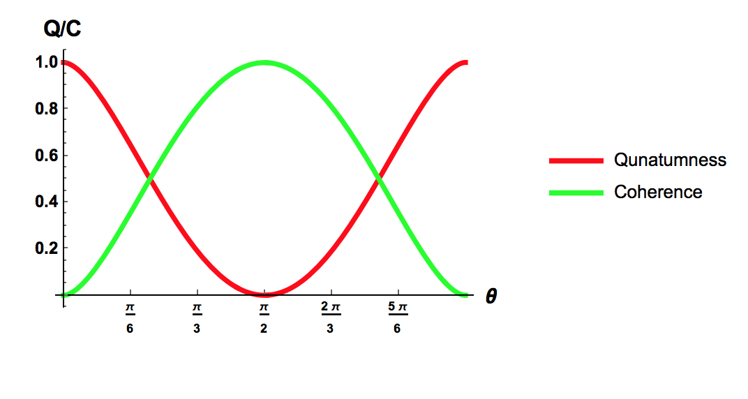
This gives rise to complementary behaviour of quantumness $Q$ and coherence $C$, as the sum will always be bounded by a positive quantity $D$ (see figure (1) as a particular example).

Note: For a qubit in particular, if we use mutually unbiased basis as observable $B$, we will always have $p^{\mathbf{{}^{\prime}}A}=\big[\frac{1}{2},\frac{1}{2}]^{T}$ and the quantity $D$ will always have value equal to one. $Q(\rho_{pure})+C(\rho_{pure})=1$. The marginal probability distribution ( $p^{A}$ ) of outcomes of A when we first observe A followed by B is, $p^{A}=\begin{bmatrix}\langle 0|\rho|0\rangle\\ \langle 1|\rho|1\rangle\\ \end{bmatrix}$. The marginal probability distribution ( $p^{\mathbf{{}^{\prime}}A}$ ) of outcomes of A, when we make a prior measurement of B, which is in a mutually unbiased basis is, $p^{\mathbf{{}^{\prime}}A}=\begin{bmatrix}\frac{1}{2}\\ \frac{1}{2}\\ \end{bmatrix}$. The quantumness of the qubit becomes, $Q(\rho_{pure})=\ \ S(p^{A}||p^{\mathbf{{}^{\prime}}A})=\ \ \langle 0|\rho|0\rangle\log\frac{\langle 0|\rho|0\rangle}{p_{1}^{{}^{\prime}}}+\langle 1|\rho|1\rangle\log\frac{\langle 1|\rho|1\rangle}{1-p_{1}^{{}^{\prime}}}=\langle 0|\rho|0\rangle\log\langle 0|\rho|0\rangle+\langle 1|\rho|1\rangle\log\langle 1|\rho|1\rangle\\ \ \ \ -\big[\langle 0|\rho|0\rangle\log p_{1}^{{}^{\prime}}+\langle 1|\rho|1\rangle\log(1-p_{1}^{{}^{\prime}})\big]-C(\rho_{pure})+\big[\langle 0|\rho|0\rangle+\langle 1|\rho|1\rangle\big]$. Therefore, the coherence and quantumness satisfy $Q(\rho_{pure})+C(\rho_{pure})=1$.

In this section, we take specific examples to study the behaviour of quantumness $Q$, by selecting various states and observables.

Quantifying the quantum nature and understanding what is quantum in a single system is of fundamental importance. Here, we show that quantumness in a single system may depend on the choice of observables for which measurements are performed. In particular, we conceptualize quantumness of the relative incompatibility of a state with respect to two non-commuting observables. We have shown that it satisfies the standard properties like convexity and additivity. Most interestingly, for a given choice of basis of a particular observable, quantumness shows complementary feature with the coherence of a system. This clearly indicates that quantumness of a state is something quite different than the quantum coherence. It is something that is only revealed in presence of two non-commuting observables. We hope that our finding adds new aspects to the notion of quantum for a single system and may be useful in quantum information processing.

References

- Ekert (1991) A. K. Ekert, Phys. Rev. Lett. 67, 661 (1991).
- Bennett and Brassard (2014) C. H. Bennett and G. Brassard, Theor. Comput. Sci. 560, 7 (2014).
- Shor and Preskill (2000) P. W. Shor and J. Preskill, Phys. Rev. Lett. 85, 441 (2000).
- Adhikari et al. (2010) S. Adhikari, I. Chakrabarty, and P. Agrawal, Quant. Inf. Comp., 12, 0253 (2012).
- Bose et al. (1998) S. Bose, V. Vedral, and P. L. Knight, Phys. Rev. A 57, 822 (1998).
- Ollivier and Zurek (2001) H. Ollivier and W. H. Zurek, Phys. Rev. Lett. 88, 017901 (2001).
- Henderson and Vedral (2001) L. Henderson and V. Vedral, Journal of Physics A: Mathematical and General 34, 6899 (2001).
- Modi et al. (2010) K. Modi, T. Paterek, W. Son, V. Vedral, and M. Williamson, Phys. Rev. Lett. 104, 080501 (2010).
- Chakrabarty et al. (2011) I. Chakrabarty, P. Agrawal, and A. K. Pati, Eur. Phys. J. D 65, 605 (2011).
- Winter and Yang (2016) A. Winter and D. Yang, Phys. Rev. Lett. 116, 120404 (2016).
- Maccone and Pati (2014) L. Maccone and A. K. Pati, Phys. Rev. Lett. 113, 260401 (2014).
- Song et al. (2017) Q.-C. Song, J.-L. Li, G.-X. Peng, and C.-F. Qiao, Scientific Reports 7, 44764 (2017).
- Wang et al. (2016) K. Wang, X. Zhan, Z. Bian, J. Li, Y. Zhang, and P. Xue, Phys. Rev. A 93, 052108 (2016).
- Mukhopadhyay et al. (2016) C. Mukhopadhyay, N. Shukla, and A. K. Pati, EPL (Europhysics Letters) 113, 50002 (2016).
- Pati et al. (2019) A. K. Pati, L.-M. Yang, C. Mukhopadhyay, S.-M. Fei, and Z.-X. Wang, arXiv preprint arXiv:1907.13067 (2019).
- Baumgratz et al. (2014) T. Baumgratz, M. Cramer, and M. B. Plenio, Phys. Rev. Lett. 113, 140401 (2014).
- Aberg (2006) J. Aberg, arXiv:quant-ph/0612146 (2006).
- Brask and Brunner (2015) J. B. Brask and N. Brunner, Phys. Rev. E 92, 062101 (2015).
- Lostaglio et al. (2015) M. Lostaglio, D. Jennings, and T. Rudolph, Nature Communications 6, 6383 (2015).
- Anand and Pati (2016) N. Anand and A. K. Pati, arXiv:1611.04542 (2016).
- Shi et al. (2017) H.-L. Shi, S.-Y. Liu, X.-H. Wang, W.-L. Yang, Z.-Y. Yang, and H. Fan, Phys. Rev. A 95, 032307 (2017).
- Olaya-Castro et al. (2008) A. Olaya-Castro, C. F. Lee, F. F. Olsen, and N. F. Johnson, Phys. Rev. B 78, 085115 (2008).
- Bera et al. (2015) M. N. Bera, T. Qureshi, M. A. Siddiqui, and A. K. Pati, Phys. Rev. A 92, 012118 (2015).
- Yuan et al. (2018) Y. Yuan, Z. Hou, Y.-Y. Zhao, H.-S. Zhong, G.-Y. Xiang, C.-F. Li, and G.-C. Guo, Optics Express 26, 4470 (2018).
- Abbott et al. (2008) D. Abbott, P. C. Davies, and A. K. Pati, Quantum aspects of life (World Scientific, 2008).
- Bandyopadhyay et al. (2012) J. N. Bandyopadhyay, T. Paterek, and D. Kaszlikowski, Phys. Rev. Lett. 109, 110502 (2012).
- Wilde et al. (2009) M. M. Wilde, J. M. McCracken, and A. Mizel, Proceedings of the Royal Society A: Mathematical, Physical and Engineering Sciences 466, 1347 (2009).
- Streltsov et al. (2015) A. Streltsov, U. Singh, H. S. Dhar, M. N. Bera, and G. Adesso, Phys. Rev. Lett. 115, 020403 (2015).
- Asbóth et al. (2005) J. K. Asbóth, J. Calsamiglia, and H. Ritsch, Phys. Rev. Lett. 94, 173602 (2005).
- Xi et al. (2015) Z. Xi, Y. Li, and H. Fan, Scientific Reports 5, 10922 (2015).
- Streltsov et al. (2016) A. Streltsov, E. Chitambar, S. Rana, M. N. Bera, A. Winter, and M. Lewenstein, Phys. Rev. Lett. 116, 240405 (2016).
- Qi et al. (2017) X. Qi, T. Gao, and F. Yan, Journal of Physics A: Mathematical and Theoretical 50, 285301 (2017).
- Chin (2017) S. Chin, Phys. Rev. A 96, 042336 (2017).
- Zhu et al. (2017) H. Zhu, Z. Ma, Z. Cao, S.-M. Fei, and V. Vedral, Phys. Rev. A 96, 032316 (2017).
- Zhu et al. (2018) H. Zhu, M. Hayashi, and L. Chen, Phys. Rev. A 97, 022342 (2018).
- Korzekwa et al. (2016) K. Korzekwa, M. Lostaglio, J. Oppenheim, and D. Jennings, New Journal of Physics 18, 023045 (2016).
- Hillery (2016) M. Hillery, Phys. Rev. A 93, 012111 (2016).
- Napoli et al. (2016) C. Napoli, T. R. Bromley, M. Cianciaruso, M. Piani, N. Johnston, and G. Adesso, Phys. Rev. Lett. 116, 150502 (2016).
- Das et al. (2018) S. Das, I. Chakrabarty, A. K. Pati, A. Sen, and U. Sen, arXiv:1812.08656 (2018).
Appendix A Additivity
We take two qubit 1 and 2 and we assume that their states are represented by and respectively. The quantumness also depends on two observables A and B. We fix both the observables to quantify the quantumness in each qubit. The marginal probability distribution ( ) of outcomes of A on qubit 1 when we first observe A followed by B is given by, Similarly, the marginal probability distribution ( ) of outcome of A on qubit 1 when we first observe B followed by A is given by, Now we extend the same idea to qubit 2. The two marginal probability distribution ( and ) corresponding to outcome of A when A was observed before B and after B is given by, , respecxtively. The quantumness of qubit 1 becomes, Similarly, the quantumness of qubit 2 becomes, The quantumness of composite system is given by, = . Here we have two independent joint probability distribution as, The quantumness of composite system becomes,