Robust Factor Analysis Parameter EstimationThanks: This work was supported by the Hong Kong RGC 16208917 research grant. Affiliation: Department of Electronic and Computer Engineering

Rui Zhou Affiliation: Department of Electronic and Computer Engineering Junyan Liu Affiliation: The Hong Kong University of Science and Technology, Hong Kong Sandeep Kumar Affiliation: E-mail {rui.zhou, jliubl}@connect.ust.hk, {eesandeep, palomar}@ust.hk Daniel P. Palomar

Abstract

This paper considers the problem of robustly estimating the parameters of a heavy-tailed multivariate distribution when the covariance matrix is known to have the structure of a low-rank matrix plus a diagonal matrix as considered in factor analysis (FA). By assuming the observed data to follow the multivariate Student’s $t$ distribution, we can robustly estimate the parameters via maximum likelihood estimation (MLE). However, the MLE of parameters becomes an intractable problem when the multivariate Student’s $t$ distribution and the FA structure are both introduced. In this paper, we propose an algorithm based on the generalized expectation maximization (GEM) method to obtain estimators. The robustness of our proposed method is further enhanced to cope with missing values. Finally, we show the performance of our proposed algorithm using both synthetic data and real financial data.

Keywords:

Robust parameter estimation Factor Analysis Student’s

t

Generalized expectation maximization Missing values.

1 Introduction

Factor analysis (FA) is of great significance in various fields like finance, statistics, and cognitive ratio [11, 14]. A basic FA model can be written as $\mathbf{x}=\boldsymbol{\mu}+\mathbf{B}\mathbf{f}+\boldsymbol{\varepsilon}$ , where $\mathbf{x}\in\mathbb{R}^{p}$ is the observed vector, $\boldsymbol{\mu}\in\mathbb{R}^{p}$ is a constant vector, $\mathbf{B}\in\mathbb{R}^{p\times r}\left(r\ll p\right)$ is the factors loading matrix, $\mathbf{f}\in\mathbb{R}^{r}$ is a vector of low-dimensional common factors, and $\boldsymbol{\varepsilon}\in\mathbb{R}^{p}$ is a vector of uncorrelated noise. For example, in a financial market, $\mathbf{x}$ can be the return of stocks, and $\mathbf{f}$ can be some macroeconomic factors like growth rate of the GDP, inflation rate, unemployment rate, etc. [2]. FA model typically assumes that $\mathbf{f}$ and $\boldsymbol{\varepsilon}$ are uncorrelated and both zero-mean, and the covariance matrix of $\mathbf{f}$ is an $r\times r$ identity matrix, denoted by $\mathbf{I}_{r}$ . Following this, the covariance matrix of $\mathbf{x}$ can be expressed as $\mathbf{\Sigma}=\mathbf{B}\mathbf{B}^{T}+\mathbf{\Psi}$ , where $\mathbf{\Psi}$ is a $p\times p$ diagonal matrix containing the variance of noise at its diagonal. Note that, with the FA structure, the number of parameters of the covariance matrix has been greatly reduced from $p\left(p+1\right)/2$ to $p\left(r+1\right)$ . Therefore, the estimation of $\mathbf{\Sigma}$ could be improved due to the FA structure.

1.1 Related Works

Learn From $\mathbf{\Sigma}$ :

A large amount of literature has focused on estimating the covariance matrix with FA structure. One choice is decomposing the estimated $\mathbf{\Sigma}$ into the sum of a low-rank matrix and a diagonal matrix, e.g., constrained minimum trace factor analysis (MTFA) [13]. But a main drawback is imposing the hard equality constraint $\mathbf{\Sigma}=\mathbf{B}\mathbf{B}^{T}+\mathbf{\Psi}$ , which does not allow any differences between $\mathbf{\Sigma}$ and $\mathbf{B}\mathbf{B}^{T}+\mathbf{\Psi}$ . Its application is restricted as the exact $\mathbf{\Sigma}$ is usually not observed. Another choice is to approximate the target matrix by a FA structured one. A naive method is to obtain $\hat{\mathbf{B}}$ firstly via principal component analysis (PCA) and then $\hat{\mathbf{\Psi}}$ by taking directly the residual’s sample variance. A joint estimation method over $\mathbf{B}$ and $\mathbf{\Psi}$ is usually chosen to minimize $\lVert\mathbf{\Sigma}-\left(\mathbf{B}\mathbf{B}^{T}+\mathbf{\Psi}\right)\rVert_{F}^{2}$ , where $\lVert\cdot\rVert_{F}$ denotes the Frobenius norm of a matrix. This problem can be solved by applying PCA iteratively [11].

Learn From Data:

Different from works mentioned above, the MLE for FA directly learns the parameters from raw data. It assumes that the data are generated from a certain statistical model, typically the multivariate Gaussian distribution, and then the parameters are estimated by maximizing the likelihood function. However, a disadvantage of the estimators under the Gaussian assumption is sensitiveness to outliers [2]. A popular way to obtain a more robust estimation result is to consider some robust heavy-tailed distribution, such as multivariate Student’s $t$ or multivariate Skew $t$ [15, 16] instead of Gaussian. The two aforementioned methods both assume that $\mathbf{f}$ and $\boldsymbol{\varepsilon}$ follow the same heavy tail distribution sharing the same degrees of freedom. As $\mathbf{f}$ and $\boldsymbol{\varepsilon}$ are not observed, such an assumption is very restrictive and difficult to verify in practice.

1.2 Contributions

This paper considers more general and practically verifiable assumptions on the FA model: we only assume that the observation $\mathbf{x}$ follows a multivariate Student’s $t$ distribution and the FA structure with no additional restrictions on $\mathbf{f}$ and $\boldsymbol{\varepsilon}$ . For this more general model, we propose an efficient algorithm to estimate the parameters based on the generalized expectation maximization (GEM) [1] method. In addition, we use the PX-EM [7] method to accelerate the GEM. Our proposed algorithm can be easily extended to other situations, e.g., when observed data contains missing values [6] or when it follows the multivariate Skew $t$ distribution. With synthetic data, our proposed algorithm shows great estimation accuracy and robustness to outliers and missing data, which is very meaningful in practical applications. We also consider real market data in the numerical results, where the global minimum variance portfolio is designed using our estimator and compared with those using other estimators.

2 Gaussian FA Problem

Given the sample covariance matrix of the observed data as $\mathbf{S}$ , the MLE problem for FA under the Gaussian distribution assumption (GFA) is given as below:

$\displaystyle\underset{\mathbf{\Sigma},\mathbf{B},\mathbf{\Psi}}{\mathsf{maximize}}$	$\displaystyle\log\lvert\mathbf{\Sigma}^{-1}\rvert-\textrm{Tr}\left(\mathbf{\Sigma}^{-1}\mathbf{S}\right)$	(1)
$\displaystyle\mathsf{subject\,\,to}$	$\displaystyle\mathbf{\Sigma}=\mathbf{B}\mathbf{B}^{T}+\mathbf{\Psi}$
	$\displaystyle\mathbf{\Psi}=\textrm{Diag}\left(\psi_{1},\dots,\psi_{p}\right)\succ\mathbf{0}.$

The solution to problem (1) would be $\mathbf{\Sigma}^{\star}=\mathbf{S}$ if the structure constraints were ignored, but becomes intractable when the FA structure is imposed. Here we introduce two algorithms for solving problem (1).

Alternating Algorithm:

Problem (1) can be solved by an alternating optimization approach, which can be performed by alternately updating $\mathbf{B}$ and $\mathbf{\Psi}$ (note that this actually corresponds to an alternating optimization over a factor model decomposition of $\mathbf{\Sigma}^{-1}$ instead of an alternating optimization over $\mathbf{B}$ and $\mathbf{\Psi}$ , cf. [9, 10]). For fixed $\mathbf{\Psi}$ , the optimal update for $\mathbf{B}$ is given next.

Lemma 1

([9]) Given a feasible $\mathbf{\Psi}$ , the optimal $\mathbf{B}^{\star}$ maximizing problem (1) is $\mathbf{B}^{\star}=\mathbf{\Psi}^{\frac{1}{2}}\mathbf{U}\mathbf{D}^{\frac{1}{2}}$ where $\mathbf{U}\mathbf{\Lambda}\mathbf{U}^{T}$ is the eigenvalue decomposition (EVD) of $\mathbf{\Psi}^{-\frac{1}{2}}\mathbf{S}\mathbf{\Psi}^{-\frac{1}{2}}$ and $\mathbf{D}=\textrm{Diag}\left(d_{1},\dots,d_{r},0,\dots,0\right)$ with $d_{i}=\max\left(\lambda_{i}-1,0\right)$ .

For fixed $\mathbf{B}$ , the update for $\mathbf{\Psi}$ is set as $\textrm{Diag}\left(\mathbf{S}-\mathbf{B}\mathbf{B}^{T}\right)$ .

MM Algorithm:

Recently, a majorization-minimization (MM) [12] based method has been proposed in [4] to obtain the optimal $\mathbf{\Sigma}$ . Plugging the optimal $\mathbf{B}^{\star}$ from Lemma 1 in (1), we can achieve a concentrated version of (1).

Lemma 2

([4]) Denoting $\mathbf{\Phi}=\mathbf{\Psi}^{-1}$ , the problem (1) is equivalent to minimizing $f\left(\boldsymbol{\phi}\right)$ , where $f\left(\boldsymbol{\phi}\right)=f_{1}\left(\boldsymbol{\phi}\right)-f_{2}\left(\boldsymbol{\phi}\right)$ with $f_{1}\left(\boldsymbol{\phi}\right)=\sum_{i=1}^{p}\left(-\log\phi_{i}+S_{ii}\phi_{i}\right)$ , $f_{2}\left(\boldsymbol{\phi}\right)=-\sum_{i=1}^{r}\left(\log\left(\max\left\{1,\lambda_{i}^{*}\right\}\right)-\max\left\{1,\lambda_{i}^{*}\right\}+1\right)$ and $\left\{\lambda_{i}^{*}\right\}_{i=1}^{r}$ are the top $r$ eigenvalues of $\mathbf{S}^{*}=\mathbf{\Phi}^{\frac{1}{2}}\mathbf{S}\mathbf{\Phi}^{\frac{1}{2}}$ . Besides, $f_{1}\left(\boldsymbol{\phi}\right)$ and $f_{2}\left(\boldsymbol{\phi}\right)$ are both convex in $\boldsymbol{\phi}$ .

By linearizing the $f_{2}\left(\boldsymbol{\phi}\right)$ using its sub-gradient, we can majorize $f\left(\boldsymbol{\phi}\right)$ by $\bar{f}\left(\boldsymbol{\phi}\right)=\sum_{i=1}^{p}\big(-\log\phi_{i}+S_{ii}\phi_{i}-\triangledown_{i}^{\left(k\right)}\phi_{i}\big)$ , where $\boldsymbol{\triangledown}^{\left(k\right)}$ is a subgradient of $f_{2}\left(\boldsymbol{\phi}\right)$ at the $k$ th iteration. The $\boldsymbol{\triangledown}^{\left(k\right)}$ can be calculated as $\triangledown_{i}^{\left(k\right)}=\big(\mathbf{\Phi}^{-\frac{1}{2}}\mathbf{U}^{*}\mathbf{D}_{1}\mathbf{U}^{*T}\mathbf{\Phi}^{\frac{1}{2}}\mathbf{S}\big)_{ii}$ where $\mathbf{U}^{*}\mathbf{\Lambda}^{*}\mathbf{U}^{*T}$ is the EVD of $\mathbf{\Phi}^{\frac{1}{2}}\mathbf{S}^{\left(k\right)}\mathbf{\Phi}^{\frac{1}{2}}$ and $\mathbf{D}_{1}=\textrm{Diag}\left(d_{1},\dots,d_{r},0,\dots 0\right)$ with $d_{i}=\max\left\{0,1-1/\lambda_{i}^{*}\right\}$ [4, 5]. Then the update of $\mathbf{\Phi}$ can be easily obtained as $\phi_{i}^{\left(k+1\right)}=\big(S_{ii}^{\left(k\right)}-\triangledown_{i}^{\left(k\right)}\big)^{-1}$ for $i=1,\dots,p$ . By iteratively taking the above procedure, we can get a converged sequence of $\boldsymbol{\phi}^{\left(k\right)}$ . Finally we can set $\mathbf{\Psi}=\mathbf{\Phi}^{-1}$ and compute $\mathbf{B}$ via Lemma 1.

It should be noted that the two algorithms are the same and can be verified by matrix algebra.

3 Problem Statement

The $p$ -dimensional multivariate Student’s $t$ distribution, denoted as $\boldsymbol{t}_{p}\left(\boldsymbol{\mu},\mathbf{\Sigma},\nu\right)$ , has the probability density function (pdf)

f\left(\mathbf{x}|\boldsymbol{\theta}\right)=\frac{\mathrm{\mathrm{\Gamma}}\left(\frac{\nu+p}{2}\right)}{\mathrm{\mathrm{\Gamma}}\left(\frac{\nu}{2}\right)\nu^{\frac{p}{2}}\pi^{\frac{p}{2}}\lvert\mathbf{\Sigma}\rvert^{\frac{1}{2}}}\left[1+\frac{1}{\nu}\left(\mathbf{x}-\boldsymbol{\mu}\right)^{T}\mathbf{\Sigma}^{-1}\left(\mathbf{x}-\boldsymbol{\mu}\right)\right]^{-\frac{\nu+p}{2}}

(2)

where $\boldsymbol{\theta}=\left(\boldsymbol{\mu},\mathbf{\Sigma},\nu\right)$ , $\nu$ is the degrees of freedom, $\mathbf{\Sigma}$ is the scale $p\times p$ positive definite matrix, $\boldsymbol{\mu}$ is the $p$ -dimensional mean vector, and $\mathrm{\mathrm{\Gamma}}\left(a\right)=\int_{0}^{\infty}t^{\left(a-1\right)}\exp\left(-t\right)dt$ is the gamma function. Note that the covariance matrix of $\mathbf{x}$ is $\frac{\nu}{\nu-2}\mathbf{\Sigma}$ , and it is not defined for $\nu\leq 2$ . Interestingly, the above multivariate Student’s $t$ distribution can be represented in a hierarchical structure as $\mathbf{x}|\tau\overset{i.i.d}{\sim}\mathcal{N}_{p}\left(\boldsymbol{\mu},\frac{1}{\tau}\mathbf{\Sigma}\right)$ with $\tau\overset{i.i.d}{\sim}\textrm{Gamma}\left(\frac{\nu}{2},\frac{\nu}{2}\right)$ , where $\mathcal{N}_{p}\left(\boldsymbol{\mu},\mathbf{\Sigma}\right)$ is the multivariate Gaussian distribution with mean vector $\boldsymbol{\mu}$ and covariance matrix $\mathbf{\Sigma}$ . $\textrm{Gamma}\left(a,b\right)$ means gamma distribution with shape $a$ and rate $b$ , whose pdf is $f\left(\tau\right)=b^{a}\tau^{\left(a-1\right)}\exp\left(-b\tau\right)/\mathrm{\mathrm{\Gamma}}\left(a\right)$ .

We consider that the observed $p$ -dimensional data $\mathbf{x}_{t},t=1,\dots,T$ follows the independent and identical distributed (i.i.d.) multivariate Student’s $t$ distribution, i.e., $\mathbf{x}_{t}\sim\boldsymbol{t}_{p}\left(\boldsymbol{\mu},\mathbf{\Sigma},\nu\right)$ . Besides, we assume that $\mathbf{x}_{t}$ follows the FA model, which means $\mathbf{\Sigma}=\mathbf{B}\mathbf{B}^{T}+\mathbf{\Psi}$ . Note that we omit a scaling factor in order to simplify the notation (recall that here $\mathbf{\Sigma}$ refers to the scale matrix). A natural approach is to obtain the parameter estimation through MLE method, i.e., maximizing $L\left(\boldsymbol{\theta}|\mathbf{X}\right)=\sum_{t}\log f\left(\mathbf{x}_{t}|\boldsymbol{\theta}\right)$ w.r.t. $\boldsymbol{\theta}$ , where $\mathbf{X}\in\mathbb{R}^{T\times p}$ with $\mathbf{x}_{t}$ along the $t$ -th row.

4 Problem Solution

It is very difficult to directly solve the above MLE problem as the objective function and constraints are both non-convex. The expectation maximization (EM) algorithm is a powerful iterative method to handle such problem [8]. By incorporating the latent data $\mathbf{Z}$ , EM can be employed to convert the maximization for $L\left(\mathbf{X}|\boldsymbol{\theta}\right)$ to the maximization for a sequence of simpler and solvable problems. In each iteration, it requires $Q(\boldsymbol{\theta}|\boldsymbol{\theta}^{\left(k\right)})$ , which is the expected log-likelihood function of $L\left(\mathbf{X}|\boldsymbol{\theta}\right)$ with respect to the current conditional distribution of $\mathbf{Z}$ given the $\mathbf{X}$ and the current estimate of the parameter $\boldsymbol{\theta}^{\left(k\right)}$ . Then it finds $\boldsymbol{\theta}^{\left(k+1\right)}$ by maximizing $Q(\boldsymbol{\theta}|\boldsymbol{\theta}^{\left(k\right)})$ . However, the computational cost of solving the subproblem might still be rather heavy and make the whole EM algorithm impractical. That is when the GEM algorithm can help. The GEM is an iterative method based on the EM philosophy but requiring an improvement at each iteration instead of a full maximization as in EM.

4.1 The RFA Algorithm

In this section, we propose a robust factor analysis (RFA) algorithm to solve the above problem. By incorporating the latent variables $\tau$ from the multivariate Student’s $t$ hierarchical structure, the log-likelihood function of the complete data $\left(\mathbf{X},\boldsymbol{\tau}\right)$ is given in (3). Note that $\boldsymbol{\tau}$ corresponds to $\mathbf{Z}$ in our application.

	$\displaystyle L\left(\boldsymbol{\theta}\|\mathbf{x},\boldsymbol{\tau}\right)$	$\displaystyle=\frac{T}{2}\log\lvert\mathbf{\Sigma}^{-1}\rvert-\frac{1}{2}\textrm{Tr}\left(\mathbf{\Sigma}^{-1}\sum_{t=1}^{T}\tau_{t}\left(\mathbf{x}_{t}-\boldsymbol{\mu}\right)\left(\mathbf{x}_{t}-\boldsymbol{\mu}\right)^{T}\right)$		(3)
		$\displaystyle+\frac{T\nu}{2}\log\frac{\nu}{2}+\frac{\nu}{2}\sum_{t=1}^{T}\left(\log\tau_{t}-\tau_{t}\right)-T\log\mathrm{\mathrm{\Gamma}}\left(\frac{\nu}{2}\right)+const.$		(3)

Expectation Step:

The expectation step of the GEM algorithm is to find the conditional expectation of $L\left(\boldsymbol{\theta}|\mathbf{X},\boldsymbol{\tau}\right)$ over $\boldsymbol{\tau}$ given the observed $\mathbf{X}$ and the current estimation of $\boldsymbol{\theta}$ , i.e., $\boldsymbol{\theta}^{\left(k\right)}$ . Since the conditional expectation of $\tau_{t}$ and $\log\tau_{t}$ for $t=1,\dots,T$ can be directly calculated as

	$\displaystyle e_{1,t}^{\left(k\right)}$	$\displaystyle=\textrm{E}\left(\tau_{t}\|\mathbf{x}_{t},\boldsymbol{\theta}^{\left(k\right)}\right)=\frac{\nu^{\left(k\right)}+p}{\nu^{\left(k\right)}+d\left(\mathbf{x}_{t},\boldsymbol{\mu}^{\left(k\right)},\mathbf{\Sigma}^{\left(k\right)}\right)}$
	$\displaystyle e_{2,t}^{\left(k\right)}$	$\displaystyle=\textrm{E}\left(\log\tau_{t}\|\mathbf{x}_{t},\boldsymbol{\theta}^{\left(k\right)}\right)=\psi\left(\frac{\nu^{\left(k\right)}+p}{2}\right)-\log\frac{\nu^{\left(k\right)}+d\left(\mathbf{x}_{t},\boldsymbol{\mu}^{\left(k\right)},\mathbf{\Sigma}^{\left(k\right)}\right)}{2}$

where $d\left(\mathbf{x},\boldsymbol{\mu},\mathbf{\Sigma}\right)=\left(\mathbf{x}-\boldsymbol{\mu}\right)^{T}\left(\mathbf{\Sigma}\right)^{-1}\left(\mathbf{x}-\boldsymbol{\mu}\right)$ is the Mahalanobis distance between $\mathbf{x}_{t}$ and $\boldsymbol{\mu}$ [6], then the expectation of the complete data log-likelihood (3) is

	$\displaystyle Q\left(\boldsymbol{\theta}\|\boldsymbol{\theta}^{\left(k\right)}\right)$	$\displaystyle=\frac{T}{2}\log\lvert\mathbf{\Sigma}^{-1}\rvert-\frac{1}{2}\textrm{Tr}\left(\mathbf{\Sigma}^{-1}\left(\sum_{t=1}^{T}e_{1,t}^{\left(k\right)}\left(\mathbf{x}_{t}-\boldsymbol{\mu}\right)\left(\mathbf{x}_{t}-\boldsymbol{\mu}\right)^{T}\right)\right)$		(4)
		$\displaystyle+\frac{T\nu}{2}\log\frac{\nu}{2}+\frac{\nu}{2}\sum_{t=1}^{T}\left(e_{2,t}^{\left(k\right)}-e_{1,t}^{\left(k\right)}\right)-T\log\mathrm{\mathrm{\Gamma}}\left(\frac{\nu}{2}\right)+const.$		(4)

Maximization Step:

Here we devide the parameters update into two parts.

Update of $\boldsymbol{\mu}$ and $\nu$ :

It is easy to see that $\boldsymbol{\mu}$ and $\nu$ are actually decoupled in $Q\big(\boldsymbol{\theta}|\boldsymbol{\theta}^{\left(k\right)}\big)$ and thus can be easily obtained by setting their derivative to zero. Then the update scheme for $\left(\boldsymbol{\mu},\nu\right)$ is

\boldsymbol{\mu}^{\left(k+1\right)}=\sum_{t=1}^{T}e_{1,t}^{\left(k\right)}\mathbf{x}_{t}\Big/\sum_{t=1}^{T}e_{1,t}^{\left(k\right)}

(5)

\nu^{\left(k+1\right)}=\underset{\nu>0}{\textrm{argmax}}\left\{\frac{T\nu}{2}\log\frac{\nu}{2}+\frac{\nu}{2}\sum_{t=1}^{T}\left(e_{2,t}^{\left(k\right)}-e_{1,t}^{\left(k\right)}\right)-T\log\mathrm{\mathrm{\Gamma}}\left(\frac{\nu}{2}\right)\right\}.

(6)

According to Proposition 1 in [6], $\nu^{\left(k+1\right)}$ always exists and can be found by bisection search. Interestingly, the update for $\boldsymbol{\mu}$ and $\nu$ are independent from each other and irrelevant to $\mathbf{\Sigma}$ .

Update of $\mathbf{\Sigma}$ :

Fixing $\boldsymbol{\mu}$ and $\nu$ , maximizing $Q\big(\boldsymbol{\theta}|\boldsymbol{\theta}^{\left(k\right)}\big)$ w.r.t. $\mathbf{\Sigma}$ is reduced to a GFA problem with $\mathbf{S}^{\left(k\right)}=\frac{1}{T}\sum_{t=1}^{T}e_{1,t}^{\left(k\right)}\left(\mathbf{x}_{t}-\boldsymbol{\mu}^{\left(k+1\right)}\right)\left(\mathbf{x}_{t}-\boldsymbol{\mu}^{\left(k+1\right)}\right)^{T}$ , which can be solved by any of the two iterative methods described in Section 2, which require several iterations until convergence. Considering that solving $\mathbf{\Sigma}$ exactly would require several iterations and could be time-consuming, we can instead only run the algorithms for one round, which would correspond to implementing the GEM instead of EM.

4.2 An Acceleration Scheme: PX-EM

A drawback of the EM algorithm is the slow convergence. The parameter expanded EM (PX-EM) [7] was proposed as an efficient method to accelerate the classical EM method and can be applied here. A well-known application of PX-EM on multivariate Student’s $t$ case is to assume that we have $\tau\overset{i.i.d}{\sim}\alpha\textrm{Gamma}\left(\frac{\nu}{2},\frac{\nu}{2}\right)$ in the Student’s $t$ hierarchical structure, where $\alpha$ is the expanded parameter.

PX-E

step: The PX-E step needs only a few modifications on the original expectation step. Specifically, the Mahalanobis distance should be calculated as $d\left(\mathbf{x}_{t},\boldsymbol{\mu}_{*},\mathbf{\Sigma}_{*}/\alpha\right)$ , where $\left(x\right)_{*}$ is the corresponding notation of $x$ in the parameter expanded statistical model.

PX-M

step: The update schemes for parameters is similar to those in EM with only few changes. The update of $\boldsymbol{\mu}$ and $\nu$ keeps unchanged but the update of $\mathbf{\Sigma}$ depends on $\left(\mathbf{S}^{\left(k\right)}\right)_{*}=\alpha^{\left(k\right)}\mathbf{S}^{\left(k\right)}$ . The update of the new parameter $\alpha$ is $\alpha^{\left(k+1\right)}=\frac{\alpha^{\left(k\right)}}{T}\sum_{t=1}^{T}e_{1,t}^{\left(k\right)}$ . After the algorithm achieves convergence, the real parameters should be recovered as $\boldsymbol{\mu}=\boldsymbol{\mu}_{*}$ , $\mathbf{\Sigma}=\mathbf{\Sigma}_{*}/\alpha$ and $\nu=\nu_{*}$ .

4.3 Robust Enhancement to Missing Data

Due to measurement problems or transmission/storage errors, the observed data $\mathbf{x}_{t}$ might contain some missing values, which has been well studied, cf. [6]. It turns out that the missing values can be regarded as latent data like $\boldsymbol{\tau}$ . The new $Q\left(\boldsymbol{\theta}|\boldsymbol{\theta}^{\left(k\right)}\right)$ at expectation step has the same expression w.r.t. $\boldsymbol{\theta}$ as in (4) [6]. Therefore the maximization step can also be achieved by first updating $\boldsymbol{\mu}$ and $\nu$ , and then $\mathbf{\Sigma}$ with FA structure imposed.

5 Numerical Experiments

5.1 Synthetic Data

We generate synthetic data following the multivariate Student’s $t$ distribution. The basic dimension setting is $p=100$ and $r=5$ . The true distribution parameters are chosen as follows: $\nu_{\textrm{true}}$ is set to be $7$ , the elements of $\boldsymbol{\mu}_{\textrm{true}}$ are drawn i.i.d. from $\mathcal{N}\left(0,1\right)$ , $\mathbf{B}_{\textrm{true}}$ comes from BARRA industry model [3] with each sector has size $20$ , diagonal elements of $\mathbf{\Psi}_{\textrm{true}}$ are generated independently from an exponential distribution with mean $10$ . The initial $\boldsymbol{\mu}^{\left(0\right)}$ , $\nu^{\left(0\right)}$ are set as the sample mean and $10$ , and $\mathbf{\Psi}^{\left(0\right)}$ , $\mathbf{B}^{\left(0\right)}$ are given by the naive PCA method. The convergence condition is set as $\lvert L^{\left(k+1\right)}-L^{\left(k\right)}\rvert\leq 10^{-6}\lvert L^{\left(k\right)}\rvert$ .

Convergence Illustration:

In Fig. 2, we compare the convergence of our proposed methods. The log-likelihood function of the observed data increases monotonically with the iterations and can finally converge. The PX-EM can significantly accelerate the convergence in this case. Then, in Fig. 2, we show the parameter estimation convergence. The parameter estimation normalized errors are defined as $\textrm{NE}\left(\boldsymbol{\mu}\right)=\lVert\hat{\boldsymbol{\mu}}-\boldsymbol{\mu}_{\textrm{true}}\rVert_{2}/\lVert\boldsymbol{\mu}_{\textrm{true}}\rVert_{2}$ , $\textrm{NE}\left(\mathbf{\Sigma}\right)=\lVert\hat{\mathbf{\Sigma}}-\mathbf{\Sigma}_{\textrm{true}}\rVert_{F}/\lVert\mathbf{\Sigma}_{\textrm{true}}\rVert_{F}$ and $\textrm{NE}\left(\nu\right)=\lvert s\left(\hat{\nu}\right)-s\left(\nu_{\textrm{true}}\right)\rvert/\lvert s\left(\nu_{\textrm{true}}\right)\rvert$ for $\boldsymbol{\mu}$ , $\mathbf{\Sigma}$ and $\nu$ , where $s\left(\nu\right)=\frac{\nu}{\nu-2}$ . In Figure 2, we can find all the errors are decreasing and finally converge.

Refer to caption — Figure 1: Optimality gap vs iterations.

Robustness Illustration:

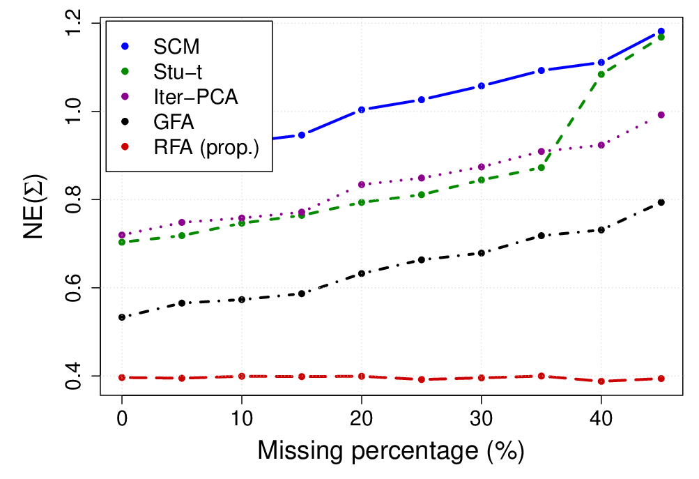
We compare our proposed RFA methods in covariance matrix estimation with sample covariance matrix (SCM), Student’s $t$ (Stu-t) estimation (without FA structure) [6], GFA, and iterative PCA (Iter-PCA) estimation. The results shown below are averaged over $100$ different realizations of $\mathbf{X}$ following Gaussian distribution. In Fig. 5, we change the sample number $n$ but fixing $p=100$ . All methods show better performance when $n$ goes large while our proposed RFA method always gives the best result. In Fig. 5, we randomly pick some rows of $\mathbf{X}$ and element-wisely add outliers drawn from $\mathcal{N}\left(0,50\right)$ . It is significant that our proposed RFA method can still hold a good estimation while the results from non-robust estimation methods are totally destroyed. The results owe to the robustness of Student’s $t$ assumption in resisting the outliers. In Fig. 5, we randomly pick some rows of $\mathbf{X}$ and randomly set $10\%$ values be missing for each row. Our proposed robust FA algorithm will be directly fed with incomplete data while for other methods we need to manually remove the rows containing the missing values. It is impressive that our proposed robust FA method can keep the lowest and almost unchanged performance.

5.2 Real Data

In this Section, we show the performance of our proposed algorithm based on the backtest with real financial data. We randomly choose $50$ stocks for $10$ times from Standard & Poor’s 500 list and 2 years ( $2\times 252$ ) continuous historical daily prices data between 01 Dec 2008 and 01 Dec 2018. Then for each resampling dataset, we perform the rolling window backtest with lookback window length set to $100$ days and test window be $5$ days. The rebalance is assumed to be done everyday without transaction cost. To fairly compare the estimation performance, we are particularly interested in the global minimum variance portfolio (GMVP): minimize $\mathbf{w}^{T}\mathbf{\Sigma}\mathbf{w}$ with constraint $\mathbf{1}^{T}\mathbf{w}=1$ , where $\mathbf{\Sigma}$ is the covariance matrix obtained from various methods. We respectively set $r=2$ and $r=4$ in Fig. 7 and 7. It turns out that our proposed RFA method can achieve smaller out-of-sample risk with less uncertainty.

Figure 6: Portfolio risk (

r=2

Figure 7: Portfolio risk (

r=4

6 Conclusion

In this paper, we have proposed the RFA algorithm to obtain the MLE of the multivariate Student’s $t$ distribution with FA structure imposed. The algorithm was based on the EM framework and had great estimation accuracy and robustness to outliers and missing values. The backtest over real financial data has shown advantages and practical usefulness of our proposed RFA algorithm.

References

[1] Dempster, A.P., Laird, N.M., Rubin, D.B.: Maximum likelihood from incomplete data via the EM algorithm. Journal of the Royal Statistical Society. Series B pp. 1–38 (1977)
[2] Feng, Y., Palomar, D.P.: A signal processing perspective on financial engineering. Foundations and Trends® in Signal Processing (2016)
[3] Heckman, L., Narayanan, S.R., Patel, S.A.: Country and industry importance in european returns. Available at SSRN 169455 (1999)
[4] Khamaru, K., Mazumder, R.: Computation of the maximum likelihood estimator in low-rank factor analysis. arXiv preprint arXiv:1801.05935 (2018)
[5] Lewis, A.S.: Derivatives of spectral functions. Mathematics of Operations Research 21(3), 576–588 (1996)
[6] Liu, C., Rubin, D.B.: ML estimation of the $t$ distribution using EM and its extensions, ECM and ECME. Statistica Sinica pp. 19–39 (1995)
[7] Liu, C., Rubin, D.B., Wu, Y.N.: Parameter expansion to accelerate EM: the PX-EM algorithm. Biometrika 85(4), 755–770 (1998)
[8] Moon, T.K.: The expectation-maximization algorithm. IEEE Signal Processing Magazine 13(6), 47–60 (1996)
[9] Ramírez, D., Santamaria, I., Van Vaerenbergh, S., Scharf, L.L.: An alternating optimization algorithm for two-channel factor analysis with common and uncommon factors. pp. 1743–1747 (2018)
[10] Santamaria, I., Scharf, L.L., Via, J., Wang, H., Wang, Y.: Passive detection of correlated subspace signals in two MIMO channels. IEEE Transactions on Signal Processing 65(20), 5266–5280 (2017)
[11] Sardarabadi, A.M., van der Veen, A.J.: Complex factor analysis and extensions. IEEE Transactions on Signal Processing 66(4), 954–967 (2018)
[12] Sun, Y., Babu, P., Palomar, D.P.: Majorization-minimization algorithms in signal processing, communications, and machine learning. IEEE Transactions on Signal Processing 65(3), 794–816 (2017)
[13] Ten Berge, J.M., Snijders, T.A., Zegers, F.E.: Computational aspects of the greatest lower bound to the reliability and constrained minimum trace factor analysis. Psychometrika 46(2), 201–213 (1981)
[14] Tsay, R.S.: Analysis of financial time series, vol. 543. John Wiley & Sons (2005)
[15] Wang, W.L., Liu, M., Lin, T.I.: Robust skew- $t$ factor analysis models for handling missing data. Statistical Methods & Applications 26(4), 649–672 (2017)
[16] Zhang, J., Li, J., Liu, C.: Robust factor analysis using the multivariate t-distribution. Statistica Sinica 24(1), 291–312 (2014)