TORM: Fast and Accurate Trajectory Optimization of
Redundant Manipulator given an End-Effector Path
Abstract
A redundant manipulator has multiple inverse kinematics solutions per end-effector pose. Accordingly, there can be many trajectories for joints that follow a given end-effector path in the Cartesian space. In this paper, we present a trajectory optimization of a redundant manipulator (TORM) to synthesize a trajectory that follows a given end-effector path accurately, while achieving smoothness and collision-free manipulation. Our method holistically incorporates three desired properties into the trajectory optimization process by integrating the Jacobian-based inverse kinematics solving method and an optimization-based motion planning approach. Specifically, we optimize a trajectory using two-stage gradient descent to reduce potential competition between different properties during the update. To avoid falling into local minima, we iteratively explore different candidate trajectories with our local update. We compare our method with state-of-the-art methods in test scenes including external obstacles and two non-obstacle problems. Our method robustly minimizes the pose error in a progressive manner while satisfying various desirable properties.
I INTRODUCTION
Remote control of various robots has been one of the main challenges in the robotics, while it is commonly used for cases where it is difficult or dangerous for a human to perform tasks [1, 2]. In this remote control scenario, a robot has to follow the task command accurately while considering its surrounding environment and constraints of the robot itself.
In the case of a redundant manipulator that this paper focuses on, a sequence of finely-specified joint configurations is required to follow the end-effector path in a Cartesian space accurately. Traditionally, inverse kinematics (IK) has been used to determine joint configurations given an end-effector pose. The traditional IK, however, cannot consider the continuity of configurations, collision avoidance, and kinematic singularities that arise when considering to follow the end-effector path.
Path-wise IK approaches [3, 4] solve this problem using non-linear optimization by considering aforementioned constraints. These approaches avoid self-collisions using a neural network, but they do not deal with collisions for external obstacles. On the other hand, prior methods [5, 6] based on motion planning approach consider external obstacles and use IK solutions to synthesize a trajectory that is following the desired path in Cartesian space. By simply using IK solutions, however, these methods have time or structural difficulties in getting a highly-accurate solution (Sec. II-B).

Main Contributions. In this work, we present a trajectory optimization of a redundant manipulator (TORM) for synthesizing a trajectory that is accurately following a given path as well as smooth and collision-free against the robot itself and external obstacles (Fig. 1). Our method incorporates these properties into the optimization process by holistically integrating the Jacobian-based IK solving method and an optimization-based motion planning approach (Sec. III-A). For the effective optimization, we consider different properties of our objectives through a two-stage update manner, which alternates making a constraint-satisfying trajectory and following a given end-effector path accurately (Sec. III-B). To avoid local minima within our optimization process, we perform iterative exploration by considering other alternative trajectories and progressively identifying a better trajectory (Sec. III-C).
To compare our method with the state-of-the-art methods, RelaxedIK [3], Stampede [4] and the work of Holladay et al. [6], we test two scenes with external obstacles and two non-obstacle problems (Sec. IV-A). Overall, we observe that our method achieves more accurate solutions given the equal planning time over the tested prior methods. Also, our method robustly minimizes the pose error reasonably fast with the anytime property, which quickly finds an initial trajectory and refines the trajectory [7] (Sec. IV-B). This result is mainly resulted by the holistic optimization process. The synthesized results of tested problems and real robot verifications can be seen in the attached video.
II RELATED WORK
In this section, we discuss prior studies in the fields of inverse kinematics and motion planning for following the desired end-effector path.
II-A Inverse Kinematics
Inverse kinematics (IK) has been studied widely to find a joint configuration from an end-effector pose [8]. In the case of a redundant manipulator, where our target robots belong to, there can be multiple joint configurations from a single end-effector pose. For this problem, several techniques for quickly finding solutions have been proposed [9, 10]. In particular, task-priority IK algorithms [11, 12, 13] prioritize solutions based on an objective function for each purpose, e.g., kinematic singularity or constraint task.
Most methods that synthesize a trajectory geometrically constrained for an end-effector pose use the Jacobian matrix for finding a feasible solution [14, 15, 16, 17]. Unfortunately, the Jacobian matrix is the first derivative of the vector-valued function with multiple variables and thus it can cause false-negative failures by getting stuck in local minima or convergence failures due to the limits of the joint angle [18].
Trac-IK [18] points out the problem and improves success rates by using randomly selected joint configurations and sequential quadratic programming. Nonetheless, its solutions do not guarantee continuity of a sequence of joint configurations to make a feasible trajectory [3]. In summary, the traditional IK approaches have different strengths and weaknesses for synthesizing a feasible trajectory.
To get alleviated solutions, many studies have present optimization techniques with objective functions for synthesizing a feasible trajectory with matching end-effector poses. Luo and Hauser [19] use a geometric and temporal optimization to generate a dynamically-feasible trajectory from a sketch input. Recently, Rakita et al. [3] proposed a real-time approach using a weighted-sum non-linear optimization, called RelaxedIK, to solve the IK problem for a sequence of motion inputs. Since the collision checking has a relatively large computational overhead, RelaxedIK uses a neural network for fast self-collision avoidance.
Based on RelaxedIK, two studies [4, 20] are proposed for synthesizing a highly-accurate trajectory on off-line. One of them is Stampede [4], which finds an optimal trajectory using a dynamic programming algorithm in a discrete-space-graph that is built by samples of IK solutions. The other work [20] generates multiple candidate trajectories from multiple starting configurations and then selects the best trajectory with a user guide by allowing a deviation if there are risks of self-collisions or kinematic singularities [20].
The aforementioned methods, called path-wise IK methods, optimize joint configurations at finely divided end-effector poses. These optimization methods synthesize an accurate and feasible trajectory satisfied with several constraints, i.e., continuity of configurations, collision avoidance, and kinematic singularities. Inspired by this strategy, we propose a trajectory optimization of a redundant manipulator (TORM) to get a collision-free and highly-accurate solution. Unlike prior path-wise IK works, however, our method considers self-collision as well as external obstacles, thanks to a tight integration of an efficient collision avoidance method using a signed distance field.
II-B Motion Planning for Following an End-effector Path
Motion planning involves a collision-free trajectory from a start configuration to a goal configuration. Based on the framework of motion planning, Holladay et al. [5, 6] present two methods to follow the desired end-effector path in Cartesian space. One [5] uses an optimization-based method, specifically Trajopt [21], by applying the discrete Fréchet distance that approximately measures the similarity of two curves. Although the optimization-based motion planning approaches quickly find a collision-free trajectory using efficient collision avoidance methods, these approaches can be stuck in local minima due to several constraints (e.g., joint limits and collisions). To assist its optimizer, this approach separately plans a trajectory by splitting the end-effector path as a set of waypoints and then sampling an IK solution at each pose.
Its subsequent work [6] points out the limitation of the prior work that is sampling only one IK solution for each pose. Considering this property, it presents a sampling-based approach that iteratively updates a layered graph by sampling new waypoints and IK solutions. However, this method needs a lot of planning time to get a highly-accurate solution, even with lazy collision checking to reduce the computational overhead.
Even though these methods find a collision-free trajectory by utilizing a motion planning approach and random IK solutions, it is hard to get a highly-accurate solution due to time or structural constraints. To overcome these difficulties, our method incorporates the Jacobian-based IK solving method into our optimization process, instead of using only IK solutions. The aforementioned path-wise IK approaches also use the objective function to minimize the end-effector pose error, but do not combine it with the objective function to avoid external obstacles. On the other hand, our approach holistically integrates these different objectives and constraints within an optimization framework, inspired by an optimization-based motion planning approach, CHOMP [22], and effectively computes refined trajectories based on our two-stage gradient descent.
III Trajectory optimization
The problem we aims to solve is finding a trajectory, , of a redundant manipulator for a given end-effector path, . The trajectory is a sequence of joint configurations, and the end-effector path, , is defined in the 6-dimensional Cartesian space.
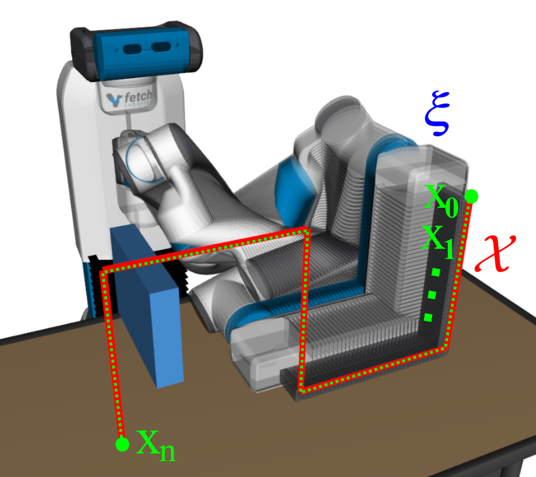
We solve the problem by applying the waypoint parameterization [23] of the path that finely splits the given end-effector path, ; is an end-effector pose. We then compute the joint configurations for end-effector poses . As a result, the trajectory is approximated as: , where is the degree of freedom (DoF) of a manipulator; is a start configuration and is a goal configuration for the computed trajectory of joint configurations. Main notations are summarized in Table I.
Our target robot is a redundant manipulator that has multiple joint configurations given an end-effector pose; if , it has infinitely many valid solutions. Among many candidates, we quickly optimize a set of joint configurations as a trajectory to follow the given end-effector path accurately, while avoiding collisions for external obstacles and the robot itself (Fig. 2).
To achieve our goal, we present a trajectory optimization of a redundant manipulator (TORM), inspired by an optimization-based motion planning approach, specifically, CHOMP [22], for finding a collision-free trajectory from the start to the goal configurations. Since CHOMP not only quickly optimizes a trajectory using gradient descent, but also efficiently avoids collisions by incorporating the objective function, we choose CHOMP as a base trajectory optimization method of our approach.
Overall, we first define our own objective function, which has a new path following objective (Sec. III-A). We repeatedly generate different trajectories (Sec. III-C), which are refined by minimizing our objective function, based on our two-stage gradient descent (Sec. III-B).
III-A Objective Function
We solve our problem by modeling an objective function holistically integrating three different properties that are 1) matching the end-effector pose, 2) avoiding collisions, and 3) achieving smoothness:
| (1) |
where is a regularization constant. is introduced to minimize the pose error between the target and current end-effector poses, and is defined using the squared Euclidean distance:
| (2) |
where computes the end-effector pose at the joint configurations using forward kinematics (FK).
quantitatively measures proximity to external obstacles using a signed distance field that can be calculated from the geometry of workspace obstacles. The robot body is simplified into spheres, which serve as conservative bounding volumes for efficient computation. Overall, can be calculated highly fast and is formulated as:
| (3) | ||||
where is partial forward kinematics, i.e., a position of a body point in the workspace at a configuration and is an obstacle cost computed from the signed distance field. At a high level, it approximately measures the sum of penetration depths between the robot body and the obstacles.
measures dynamical quantities, i.e., the squared sum of derivatives to encourage the smoothness between joint configurations:
| (4) |
| Notation | Description |
|---|---|
| Target end-effector poses that are finely divided from | |
| the given end-effector path | |
| Set of joint configurations corresponding to | |
| Joint configuration on the trajectory | |
| at -th end-effector pose | |
| Jacobian matrix, i.e., | |
| Set of body points in the workspace approximating | |
| the geometric shape of the manipulator | |
| Partial forward kinematics from the manipulator base to | |
| a body point at a configuration |
III-B Two-Stage Gradient Descent Update
We iteratively update the trajectory to minimize the cost of the objective function consisting of three different terms. To minimize the cost, our update rule is based on the gradient descent technique adopted in many optimization methods. The functional gradient of the obstacle term, , pushes the robot out of obstacles, and the functional gradient of the smooth term, , keeps the continuity between joint configurations.
Both and are responsible for synthesizing a feasible trajectory, whereas the functional gradient of the pose term, , is responsible for matching the end-effector poses . Even though we can update the trajectory by considering the three functional gradients simultaneously, we found that it can lead to conflicts between each functional gradient.
To alleviate this problem, we present a two-stage gradient descent (TSGD) that consists of two parts of updating to make a feasible trajectory and updating the trajectory to match closer to . The TSGD is repeated in which each odd iteration updates the trajectory using and , and in which even iteration updates the trajectory using :
| (5) |
where is a learning rate, and is from an equally transformed representation of the smooth term, ; acts to retain smoothness and to accelerate the optimization by having a small amount of impact on the overall trajectory [22]. Since and have a correlation between consecutive joint configurations, it is effective for updating the trajectory with covariant gradient descent using . On the other hand, does not consider consecutive joint configurations, thus we do not use . We set TSGD to perform iterative updates for refining a trajectory on average.
Our goal is to avoid collisions and to follow the given end-effector path in the Cartesian workspace, while we achieve the goal through the manipulation of joint configurations in the configuration space (C-space). As a result, while and are computed in workspace using FK, and should be defined in C-space for calculating the change of joint configurations.
Since of Eq. 2 can be represented as , we can derive the functional gradient of the pose term, , by the following:
| (6) |
where is the Jacobian matrix.
can be derived as the following [22]:
| (7) |
where is equal to , to , is the normalized velocity vector, and is the curvature vector. Since is already represented in C-space, is represented simply as .
Once a start configuration is given, we iteratively update from its next configuration, , to the goal configuration , based on our TSGD. In our problem, however, the start configuration may not be given, while an end-effector path is given.
III-C Iterative Exploration with Local Update
We can optimize a trajectory based on our update rule (Sec. III-B), but there is a probability that the updated trajectory is sub-optimal due to the local natures of our update method. Furthermore, there can be many surrounding local minima in our solution space, since we incorporate three different properties of constraints into the objective function.
To avoid getting stuck in local minima, we perform iterative exploration with local updates. Note that a redundant manipulator can have multiple joint configurations at a single pose, thus we can construct many candidate trajectories. By utilizing this property, we generate different new trajectories, which are locally refined based on our two-stage gradient descent (Sec. III-B).
Our algorithm iteratively performs two parts: exploring a new trajectory, , and locally refining the trajectory. When a new trajectory that is also locally refined has a lower cost to the existing one, we use it to the current trajectory; if the new trajectory violates the constraints, we reject it and thus do not use it as the current trajectory (Sec. III-D). The update part locally refines the trajectory using our two-stage gradient descent (Sec. III-B). This process continues until satisfying a given condition, e.g., running time or cost.

Exploring and generating a new trajectory. Each exploration part generates a new trajectory . We strive for finding a potentially good trajectory for our local optimization, which considers our objectives with smoothness, avoiding obstacles, and following a given path. Because merely connecting start and goal configuration can result in a sub-optimal solution, especially in cases of complex scenarios (e.g., Fig. 3 and environments with external obstacles) [5].
Overall, we consider random configurations and choose one that minimizes our objective function in a greedy manner for generating an initial trajectory. As the first step, we extract sub-sampled poses, , at intervals from the end-effector poses , since working with more poses tends to increase the complexity of generating a trajectory (Fig. 3); we set to . In the next step, we find suitable joint configurations at the sub-sampled poses. For the first sub-sampled pose as the start end-effector pose , we simply compute a random IK solution at the pose, if a start configuration is not given. For its next pose, we compute random IK solutions at the pose and greedily select one that minimizes our objective function when connecting it with the configuration of the previous pose; we set to . Lastly, we connect chosen joint configurations through linear interpolation for generating a new trajectory, which is then locally refined by our two-stage gradient descent.
III-D Trajectory Constraints
During the optimization process, we may find a low cost solution, but it can violate several constraints. For example, a trajectory can have collisions with obstacles or self-collisions, even though the trajectory accurately follows the given end-effector pose. Hence, we check collisions every time we find a better trajectory during our iterative exploration.
In addition to the collision checking, a manipulator commonly has several constraints that are satisfying lower and upper limits of joints, velocity limits, and kinematic singularities for joints. In the case of lower and upper limits of joints, it is traditionally handled by performing projection that resets the violating joints value to its limit value. To retain smoothness, we use a smooth projection used by CHOMP [22] during the update process. The smooth projection uses the Riemannian metric . In other words, an updated trajectory, , is defined as , where is the vector of joint values, and is a scale constant. This process is repeated until there is no violation.
For other constraints like the velocity limit, we check them together while checking collisions. The velocity limit for joints is checked by computing the velocities of joints between and for a given time interval, . Another constraint is the kinematic singularity that is a point where the robot is unstable, and it can occur when the Jacobian matrix loses full rank. To check kinematic singularities, we use the manipulability measure [24] used by RelaxedIK [3]. At a high level, it avoids making the manipulability measure less than a certain value that is computed by random samples. Note that our method returns the lowest cost trajectory guaranteed through checking constraints for constructing a feasible trajectory.


IV Experiments and Analysis
We use the Fetch robot, whose manipulator arm has 7-DoF for various tests. We report the average performance by performing tests with a machine that has 3.4 GHz Intel i7-6700 CPU and 16 GB RAM. Also, we set = , = , = and = , where is the number of the end-effector poses .
In this setting, the two-stage gradient descent, generating new trajectory, and checking constraints of our method take 67%, 32%, and 1% of the overall running time; the two-stage gradient descent is frequently iterated to refine the trajectory, as the main update operation.
In this experiment, we compute the distance between end-effector poses using a weight sum of the Euclidean distances of the translational and rotational parts, which was used in the work of Holladay et al. [6]; the weight of the rotational distance over the translational distance is .
Results with the real Fetch robot is shown in the accompanying video.
IV-A Experiment setting
We prepare two problems with external obstacles and two non-obstacle problems to evaluate and compare our method with state-of-the-art methods, RelaxedIK [3], Stampede [4], and the work of Holladay et al. [6]. In this section, we call the work of Holladay et al. [6] EIGS taken from their paper title.
Two problems with obstacles (Fig. 4) are the square tracing with the table and the “S” tracing with the table and blue box. At these problems, we do not test for RelaxedIK and Stampede, since these prior methods did not consider external obstacles. To compare ours against those prior methods, we prepare two non-obstacle problems, rotating degrees in the direction of pitch and yaw, and writing “hello” (Fig. 5), by adapting problems used in those methods; we just change writing “icra” to “hello”.
In two problems including external obstacles, we fix the start configuration located close to the obstacles, as shown the Fig. 4(b) and Fig. 4(d). On the other hand, we do not fix the start configuration for non-obstacle problems.
We used the code of RelaxedIK and Stampede that are provided by authors through their websites. For RelaxedIK, Stampede, and our method, the end-effector paths of all problems are finely divided and are fed into all the tested methods; in our experiment, the distance between two divided end-effector poses is about , following the protocol adopted in [4]. On the other hand, EIGS initially splits the end-effector path and gradually breaks down the path during the planning.
| Pose error | TL | IST | PT | ||||
| Average | Min. | Max. | |||||
| Square tracing | EIGS | 5.99e-3 | 3.92e-3 | 8.68e-3 | 23.2 | 7.1 | 50 |
| w/ obs. (n = 304) | Ours | 1.91e-5 | 1.01e-5 | 7.65e-5 | 9.5 | 5.2 | |
| “S” tracing | EIGS | 6.50e-3 | 4.56e-3 | 1.06e-2 | 20.5 | 7.0 | 50 |
| w/ obs. (n = 300) | Ours | 2.40e-5 | 6.08e-6 | 8.50e-5 | 7.8 | 5.2 | |
| Rotation task | RelaxedIK | 5.36e-2 | 4.13e-2 | 1.90e-1 | 11.1 | - | 5.2 |
| w/o obs. | Stampede | 9.42e-5 | 8.72e-5 | 9.95e-5 | 12.2 | 43 | |
| (n = 208) | EIGS | 1.07e-2 | 7.53e-3 | 1.82e-2 | 16.0 | 11 | 43 |
| Ours | 7.99e-5 | 6.83e-5 | 1.21e-4 | 13.8 | 1.8 | ||
| Writing “hello” | RelaxedIK | 5.25e-2 | 4.86e-2 | 5.99e-2 | 22.1 | - | 15 |
| w/o obs. | Stampede | 5.21e-5 | 4.93e-5 | 6.03e-5 | 24.2 | 50 | |
| (n = 496) | EIGS | 2.02e-2 | 1.71e-2 | 2.36e-2 | 35.2 | 24 | 50 |
| Ours | 5.11e-5 | 4.77e-5 | 6.38e-5 | 26.4 | 5.2 | ||
- 1
TL: Trajectory length (rad). IST: Initial solution time (s). PT: Planning time (s).
IV-B Evaluation
We mainly evaluate whether the synthesized trajectory accurately follows the given end-effector path. Note that reported results were extracted from feasible trajectories satisfying the given constraints (Sec. III-D).
Fig. 6 and Table II show the overall results for different methods. Fig. 6 shows the trajectory quality of different methods, as we have more planning time up to the maximum planning budget of seconds. On the other hand, Table II shows a snaptshot result of the trajetory computed at the maximum planing time budget. For the rotation task with obstacles, we report results by seconds, which is the initial solution time of Stampede, instead of seconds; within seconds, Stampede computed only a single trajectory at seconds. Note that in the case of RelaxedIK, a real-time planner, it quickly synthesizes one trajectory at one execution, but its computed trajectory tends to be low-quality.
Comparison with state-of-the-art methods. Fig. 6 shows how different methods compute a trajectory. EIGS and our method are improving its quality as we have more planning time, since they have the anytime property.
EIGS refines a trajectory by progressively sampling new waypoints and IK solutions. Nonetheless, our method improves the quality of the trajectory over EIGS, as we have more planning time (Fig. 6). This improvement is mainly because our method incorporates the IK solving method into the optimization process (Eq. 6), instead of simply using IK solutions.
In Table II, EIGS shows the longest length of the computed trajectory on average for all problems; we measure the length of a trajectory using the Euclidean distance. EIGS does not consider the distance in C-space, since it only check the similarity measure of two curves using the discrete Fréchet distance [6]. On the other hand, other methods take into account the smoothness between joint configurations and thus generate shorter trajectories than EIGS.
Stampede is also a sampling-based approach like EIGS, but it generates a highly-accurate solution on average (Table II). Stampede does not deal with external obstacles, but uses a neural network to check self-collision quickly. However, it takes a long time to get an initial solution, because it has to samples IK solutions at all the end-effector poses (Table II). These results show that Stampede and EIGS have different pros and cons. Nevertheless, our method shows anytime property as well as highly-accurate solutions (Fig. 6).
RelaxedIK is a real-time planner, thus it quickly finds a solution (Table II). However, its accuracy is much lower than other methods; see Fig. 5 and Fig. 6. In conclusion, RelaxedIK shows real-time performance by quickly optimizing the joint configuration for one pose, but it is difficult to obtain a highly-accurate trajectory.
Overall, our method finds an initial solution quite quickly with a high pose error, but improves its quality as we have more planning time (Fig. 6). Also, our method has a lower pose error on average than other methods, as shown in Table II. These results support that our optimization process efficiently reduces the pose error, while satisfying several constraints. The max. pose errors of our method are lower than others, except Stampede. Since our algorithm has randomness when we get IK solutions at sub-sampled poses, its max. errors can be higher than Stampede. Fortunately, our method shows the smallest min. error, resulting in the best accuracy on average. This is thanks to the fast computation of the functional gradient of our objectives, leading to find a highly-accurate solution escaping from local minima given the planning time.
| Pose error | TL | IST | PT | ||||
| Average | Min. | Max. | |||||
| Square | Ours w/o TSGD | 2.46e-3 | 2.19e-3 | 2.84e-3 | 9.2 | 5.2 | 50 |
| tracing | Ours w/o IE | 1.67e-4 | 1.29e-5 | 2.48e-3 | 9.7 | 5.2 | |
| w/ obs. | Ours | 1.91e-5 | 1.01e-5 | 7.65e-5 | 9.5 | 5.2 | |
| “S” | Ours w/o TSGD | 2.37e-3 | 1.75e-3 | 3.78e-3 | 8.1 | 5.2 | 50 |
| tracing | Ours w/o IE | 1.56e-3 | 1.12e-5 | 2.75e-2 | 7.7 | 5.2 | |
| w/ obs. | Ours | 2.40e-5 | 6.08e-6 | 8.50e-5 | 7.8 | 5.2 | |
| Rotation | Ours w/o TSGD | 9.87e-3 | 1.95e-3 | 1.87e-2 | 12.1 | 2.4 | 50 |
| task | Ours w/o IE | 8.66e-3 | 7.01e-5 | 1.65e-2 | 14.3 | 1.8 | |
| w/o obs. | Ours | 7.67e-5 | 6.72e-5 | 9.87e-5 | 13.9 | 1.8 | |
| Writing | Ours w/o TSGD | 9.68e-3 | 9.25e-3 | 1.04e-2 | 25.4 | 5.3 | 50 |
| “hello” | Ours w/o IE | 5.99e-4 | 5.07e-5 | 9.83e-3 | 27.0 | 5.2 | |
| w/o obs. | Ours | 5.11e-5 | 4.77e-5 | 6.38e-5 | 26.4 | 5.2 | |
- 1
TL: Trajectory length (rad). IST: Initial solution time (s). PT: Planning time (s).
Ablated methods for our method. To see the benefits of our proposed methods, we conduct ablabation study of our method by disabling the two-stage gradient descents (TSGD) and instead updating three functional gradients at once. We also test our methods without the iterative exploration (IE) that just tests a single trajectory updated by TSGD.
The results of ablated methods for our method show a similar performance trend regardless of external obstacles. Also, all of the methods find an initial solution almost at a similar time (Fig. 6). Excluding the TSGD has a higher pose error on average than our full method, and also has the highest min. pose error among tests, compared to other ablated methods (Table III). These results demonstrate that the different functional gradients conflict with each other. Therefore, the TSGD prevents the competition of different functional gradients and is useful to get a highly-accurate solution.
Fig. 6 shows that excluding the IE (the sky-blue line) does not reduce the pose error after certain seconds (e.g., seconds in Fig. 6(d)). This is because it was stuck in a local minimum and thus did not find a better solution as we have more planning time. As a result, excluding the IE has the largest difference between the min. and max. pose errors, as shown in Table III.
In conclusion, these results show that our method with the TSGD and IE synthesizes highly-accurate trajectories, while effectively getting out of local minima.
V Conclusion and Limitations
In this paper, we have presented the trajectory optimization of a redundant manipulator (TORM) that holistically incorporates three important properties into the trajectory optimization process by integrating the Jacobian-based IK solving method and an optimization-based motion planning approach. Given different properties, we have suggested the two-stage gradient descent to follow a given end-effector path and to make a feasible trajectory. We have also performed iterative exploration to avoid local minima. We have shown the benefits of our method over the state-of-the-art techniques in environments w/ and w/o external obstacles. Our method has robustly minimized the pose error in a progressive manner and achieved the highly-accurate trajectory at a reasonable time compared to other methods. Further, we have verified the feasibility of our synthesized trajectory using the real, Fetch manipulator.
While our method finds an accurate solution reasonably fast, there is no theoretical analysis of the error reduction rate of our approach. While the theoretical analysis could be challenging, it would shed light on deeply understanding the proposed approach in various aspects. Finally, we would like to efficiently handle dynamic environments by computing signed distance functions in real-time.
Acknowledgment
We would like to thank anonymous reviewers for constructive comments. This work was supported by SW Starlab program (IITP-2015-0-00199) and NRF/MSIT (No.2019R1A2C3002833).
References
- [1] Kapil D Katyal, Christopher Y Brown, Steven A Hechtman, Matthew P Para, Timothy G McGee, Kevin C Wolfe, Ryan J Murphy, Michael DM Kutzer, Edward W Tunstel, Michael P McLoughlin, et al., “Approaches to robotic teleoperation in a disaster scenario: From supervised autonomy to direct control”, in IEEE/RSJ International Conference on Intelligent Robots and Systems. IEEE, 2014, pp. 1874–1881.
- [2] Philip Long, Tarik Keleştemur, Aykut Özgün Önol, and Taşkin Padir, “optimization-based human-in-the-loop manipulation using joint space polytopes”, in IEEE International Conference on Robotics and Automation. IEEE, 2019, pp. 204–210.
- [3] Daniel Rakita, Bilge Mutlu, and Michael Gleicher, “RelaxedIK: Real-time synthesis of accurate and feasible robot arm motion.”, in Robotics: Science and Systems, 2018.
- [4] Daniel Rakita, Bilge Mutlu, and Michael Gleicher, “STAMPEDE: A discrete-optimization method for solving pathwise-inverse kinematics”, in IEEE International Conference on Robotics and Automation. IEEE, 2019, pp. 3507–3513.
- [5] Rachel M Holladay and Siddhartha S Srinivasa, “Distance metrics and algorithms for task space path optimization”, in IEEE/RSJ International Conference on Intelligent Robots and Systems. IEEE, 2016, pp. 5533–5540.
- [6] Rachel Holladay, Oren Salzman, and Siddhartha Srinivasa, “Minimizing task-space fréchet error via efficient incremental graph search”, IEEE Robotics and Automation Letters, vol. 4, no. 2, pp. 1999–2006, 2019.
- [7] Sertac Karaman, Matthew R Walter, Alejandro Perez, Emilio Frazzoli, and Seth Teller, “Anytime motion planning using the rrt”, in IEEE International Conference on Robotics and Automation. IEEE, 2011, pp. 1478–1483.
- [8] Samuel R Buss, “Introduction to inverse kinematics with jacobian transpose, pseudoinverse and damped least squares methods”, IEEE Journal of Robotics and Automation, vol. 17, no. 1-19, pp. 16, 2004.
- [9] Rosen Diankov, “Automated construction of robotic manipulation programs”, 2010.
- [10] Anirban Sinha and Nilanjan Chakraborty, “Geometric search-based inverse kinematics of 7-dof redundant manipulator with multiple joint offsets”, in IEEE International Conference on Robotics and Automation. IEEE, 2019, pp. 5592–5598.
- [11] Pasquale Chiacchio, Stefano Chiaverini, Lorenzo Sciavicco, and Bruno Siciliano, “Closed-loop inverse kinematics schemes for constrained redundant manipulators with task space augmentation and task priority strategy”, The International Journal of Robotics Research, vol. 10, no. 4, pp. 410–425, 1991.
- [12] Stefano Chiaverini, “Singularity-robust task-priority redundancy resolution for real-time kinematic control of robot manipulators”, IEEE Transactions on Robotics and Automation, vol. 13, no. 3, pp. 398–410, 1997.
- [13] Oussama Kanoun, Florent Lamiraux, and Pierre-Brice Wieber, “Kinematic control of redundant manipulators: Generalizing the task-priority framework to inequality task”, IEEE Transactions on Robotics, vol. 27, no. 4, pp. 785–792, 2011.
- [14] Mike Stilman, “Task constrained motion planning in robot joint space”, in IEEE/RSJ International Conference on Intelligent Robots and Systems. IEEE, 2007, pp. 3074–3081.
- [15] Dmitry Berenson, Siddhartha S Srinivasa, Dave Ferguson, and James J Kuffner, “Manipulation planning on constraint manifolds”, in IEEE International Conference on Robotics and Automation. IEEE, 2009, pp. 625–632.
- [16] Nikolaus Vahrenkamp, Dmitry Berenson, Tamim Asfour, James Kuffner, and Rüdiger Dillmann, “Humanoid motion planning for dual-arm manipulation and re-grasping tasks”, in IEEE/RSJ International Conference on Intelligent Robots and Systems. IEEE, 2009, pp. 2464–2470.
- [17] Tobias Kunz and Mike Stilman, “Manipulation planning with soft task constraints”, in IEEE/RSJ International Conference on Intelligent Robots and Systems. IEEE, 2012, pp. 1937–1942.
- [18] Patrick Beeson and Barrett Ames, “TRAC-IK: An open-source library for improved solving of generic inverse kinematics”, in IEEE International Conference on Humanoid Robots. IEEE, 2015, pp. 928–935.
- [19] Jingru Luo and Kris Hauser, “Interactive generation of dynamically feasible robot trajectories from sketches using temporal mimicking”, in IEEE International Conference on Robotics and Automation. IEEE, 2012, pp. 3665–3670.
- [20] Pragathi Praveena, Daniel Rakita, Bilge Mutlu, and Michael Gleicher, “User-guided offline synthesis of robot arm motion from 6-dof paths”, in IEEE International Conference on Robotics and Automation. IEEE, 2019, pp. 8825–8831.
- [21] John Schulman, Jonathan Ho, Alex X Lee, Ibrahim Awwal, Henry Bradlow, and Pieter Abbeel, “Finding locally optimal, collision-free trajectories with sequential convex optimization”, in Robotics: Science and Systems. Citeseer, 2013, vol. 9, pp. 1–10.
- [22] Matt Zucker, Nathan Ratliff, Anca D Dragan, Mihail Pivtoraiko, Matthew Klingensmith, Christopher M Dellin, J Andrew Bagnell, and Siddhartha S Srinivasa, “CHOMP: Covariant hamiltonian optimization for motion planning”, The International Journal of Robotics Research, vol. 32, no. 9-10, pp. 1164–1193, 2013.
- [23] Tamar Flash and Renfrey B Potts, “Communication: Discrete trajectory planning”, The International Journal of Robotics Research, vol. 7, no. 5, pp. 48–57, 1988.
- [24] Tsuneo Yoshikawa, “Manipulability of robotic mechanisms”, The International Journal of Robotics Research, vol. 4, no. 2, pp. 3–9, 1985.