跳到论文正文
W Papers独立论文阅读器 arXiv:1909.12509 论文正文 计算阅读时间 · 0%
引用这篇论文根据当前论文元数据生成,正式投稿前建议核对。


License: arXiv.org perpetual non-exclusive license
arXiv:1909.12509v3 [hep-ph] 25 Jan 2020

Study on possible molecular states composed of Λc​D¯\Lambda_{c}\bar{D} (Λb​B\Lambda_{b}B) and Σc​D¯\Sigma_{c}\bar{D} (Σb​B\Sigma_{b}B) within the Bethe-Salpeter framework

Hong-Wei Ke1 , Mei Li1, Xiao-Hai Liu1 and Xue-Qian Li2 Note: Corresponding author, khw020056@tju.edu.cn Note: xiaohai.liu@tju.edu.cn Note: lixq@nankai.edu.cn Affiliation: 1 School of Science, Tianjin University, Tianjin 300072, China
2 School of Physics, Nankai University, Tianjin 300071, China
Abstract

Pc​(4312)P_{c}(4312) observed by the LHCb collaboration is confirmed as a pentaquark and its structure, production, and decay behaviors attract great attention from theorists and experimentalists. Since its mass is very close to sum of Σc\Sigma_{c} and D¯\bar{D} masses, it is naturally tempted to be considered as a molecular state composed of Σc\Sigma_{c} and D¯\bar{D}. Moreover, Pc​(4312)P_{c}(4312) is observed in the channel with J/ψ​pJ/\psi p final state, requiring that isospin conservation Pc​(4312)P_{c}(4312) is an isospin-1/2 eigenstate. In literature, several groups used various models to estimate its spectrum. We systematically study the pentaquarks within the framework of the Bethe-Salpeter equation; thus Pc​(4312)P_{c}(4312) is an excellent target because of the available data. We calculate the spectrum of Pc​(4312)P_{c}(4312) in terms of the Bethe-Salpter equations and further study its decay modes. Some predictions on other possible pentaquark states that can be tested in future experiments are made.

pacs
12.39.Mk, 12.40.-y ,14.40.Nd

I Introduction

Due to the innovation of experimental techniques and facilities as well as the advances in theory of recent years several exotic states have been experimentally observed and theoretically studied. Indeed, more constituents would cause more ambiguities, unlike the simplest q​q¯q\bar{q} for mesons and q​q​qqqq for baryons. The inner structures of the exotic states are still not clear yet, those discoveries stir up large numbers of discussionsChen:2016spr. Indeed the theoretical exploration is crucial for getting a better understanding of the quark model and obtaining valuable information about non-perturbative physics. Definitely, to complete the theoretical job achieving more accurate data would compose the key.

Some hidden charm or bottom states were measured in two-meson final statesChoi:2003ue; Abe:2007jn; Choi:2005; Choi:2007wga; Aubert:2005rm; Ablikim:2013emm; Ablikim:2013wzq; Ablikim:2013mio; Liu:2013dau; Collaboration:2011gja. They are regarded as tetraquark states or meson-meson molecular states. In 2003 a baryon was measured by LEPSNakano:2003qx which was conjectured as a pentaquark, however later the allegation was negated by further more accurate experiments. Breaking the frustration on existence of pentaquark which was predicted by Gell-Mann in his first paper on quark model, the LHCb collaboration reported two pentaquark states observed in Λb\Lambda_{b} decays where peaks appear at the J/ψ​pJ/\psi p final statesAaij:2015tga.

Recently another narrow pentaquark state Pc​(4312)P_{c}(4312)Aaij:2019vzc has also been observed in the J/ψ​pJ/\psi p mass spectrum. Its mass and width are 4311.9±0.7−0.6+6.84311.9\pm 0.7^{+6.8}_{-0.6} MeV and 9.8±2.7−4.5+3.79.8\pm 2.7^{+3.7}_{-4.5} MeV respectively. Since its mass is very close to the sum of Σc\Sigma_{c} and D¯\bar{D} masses, it is natural to regard it as a molecular state of Σc​D¯\Sigma_{c}\bar{D}Chen:2019bip; Liu:2019tjn; Xiao:2019aya; Liu:2019zvb; He:2019ify; Xiao:2019mst; Zhang:2019xtu; Wang:2019hyc; Xu:2019zme; Wang:2019got; Chen:2019asm; Lin:2019qiv. Furthermore its width is rather wide in accordance with the property of molecular states, so the phenomenon further supports the proposal of its molecular structure. Some other theorists conjecture Pc​(4312)P_{c}(4312) as a compact pentaquark.Cheng:2019obk; Wang:2019got instead. In Ref. Fernandez-Ramirez:2019koa the authors think the interaction between Σc\Sigma_{c} and D¯\bar{D} is too weak to bind them into a bound state. It is worth deeper explorations about whether the molecule picture is reasonable. In this work we will calculate the mass spectrum of Pc​(4312)P_{c}(4312) based on the assumption that it is a stable bound state of Σc\Sigma_{c} and D¯\bar{D}. Additionally we also study other possible bound states of Λc​D¯\Lambda_{c}\bar{D}, Λb​B\Lambda_{b}B and Σb​B\Sigma_{b}B and see if they can be formed.

We will employ the Bethe-Salpeter (B-S) equation to study the possible bound state which consists of a baryon and a meson. The B-S equation is a relativistic equation to deal with the bound state and established on the basis of quantum field theorySalpeter:1952ib. Initially, people used the B-S equation to study the bound state of two fermionsChang:2004im; Chang:2005sd and the system of one-fermion-one-bosonGuo:1998ef. In Ref.Guo:2007mm; Feng:2011zzb the authors employed the Bethe-Salpeter equation to study the K​K¯K\bar{K} and B​K¯B\bar{K} molecular states and their decays. With the same approach we studied the molecular state of B​πB\piKe:2018jql, D(∗)​D(∗)D^{(*)}D^{(*)} and B(∗)​B(∗)B^{(*)}B^{(*)}Ke:2012gm. Recently the approach is extended to explore double charmed baryonsWeng:2010rb; Li:2019ekr and pentaquarks which are assumed to be two-body bound systems. In Ref.Wang:2019krq the authors studied possible bound states of Λ\Lambda (Σ\Sigma) and K¯\bar{K}. In this work we will employ a similar approach to study the possible bound states of Σc​D¯\Sigma_{c}\bar{D}, Λc​D¯\Lambda_{c}\bar{D}, Λb​B\Lambda_{b}B and Σb​B\Sigma_{b}B.

At present, pentaquark states Pc​(4312)P_{c}(4312), Pc​(4380)P_{c}(4380), Pc​(4440)P_{c}(4440) and Pc​(4457)P_{c}(4457) have been measured in decays of Λb\Lambda_{b} where the pentaquark states peak up at the invariant mass spectrum of J/ψ​pJ/\psi p, so their isospin is 12\frac{1}{2} because of isospin conservation. Thus we require that the two hadron constituents reside in an isospin eigenstate. Instead, for the Λc​D¯\Lambda_{c}\bar{D} (as well Λb​B\Lambda_{b}B) system its isospin must be 12\frac{1}{2} but the Σc​D¯\Sigma_{c}\bar{D} ( or Σb​B\Sigma_{b}B) system may reside in either isospin 12\frac{1}{2} or 32\frac{3}{2}. Certainly, for a bound system with spin-parity 12−\frac{1}{2}^{-} the two constituents are in the SSwave.

For carrying on our calculation the interactions between two constituents are needed. According to the quantum field theory two particles interact via exchanging certain mediate particles. Since two constituents in a pentaquark are color-singlet hadrons the exchanged particles are some light hadrons such as ρ\rho or (and) ω\omega etc.. The effective interactions are deduced from the chiral LagrangianRonchen:2012eg; Shen:2016tzq; He:2017aps which we list in Appendix A. With the effective interactions we obtain the kernel and establish the corresponding B-S equation.

With a reasonable parameter set, the B-S equation is solved. For a spin-isospin eigenstate, if the equation does not possess a solution, then we would conclude that the corresponding bound state should not exist in nature; on the contrary, a solution of the B-S equation implies the bound state being formed. At the same time the B-S wave function is obtained and we are able to use the corresponding formula for calculating the rates of strong decay Pc​(4312)→proton+𝒱P_{c}(4312)\to{\rm proton}+\mathcal{V} (vector) which can be compared with the data.

This paper is organized as follows: after this introduction we will derive the B-S equations related to possible bound states composed of a baryon and a meson and the formula for its strong decays. Then in section III we will solve the B-S equation numerically and present our results by figures and tables. Section IV is devoted to a brief summary.

II The bound states of Λc​D¯\Lambda_{c}\bar{D} and Σc​D¯\Sigma_{c}\bar{D}

Refer to caption
(a)  
Refer to caption
(b)  
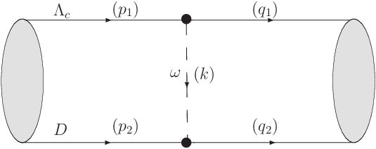
Figure 1: the bound states of Λc​D¯\Lambda_{c}\bar{D} (a) and Σc​D¯\Sigma_{c}\bar{D} (b)formed by exchanging light vector meson(s) .

Since the newly found pentaquarks Pc​(4312)P_{c}(4312), Pc​(4380),Pc​(4440)P_{c}(4380),P_{c}(4440) and Pc​(4457)P_{c}(4457) are all hadrons containing hidden charms(or hidden bottoms) and their masses are close to the sums of the masses of several real hadrons, we will focus on the molecular structures composed of one charmed (bottomed) baryon and an anti-charmed(anti-bottomed) meson. Concretely, in this paper we study Λc​D¯\Lambda_{c}\bar{D}, Σc​D¯\Sigma_{c}\bar{D}, Λb​B\Lambda_{b}B and Σb​B\Sigma_{b}B systems whose spin-parity is 12−\frac{1}{2}^{-} i.e. the spatial wave function is in SSwave. In this section as an example we only formulate the corresponding quantities for Λc​D¯\Lambda_{c}\bar{D} and Σc​D¯\Sigma_{c}\bar{D} systems. These formulas can be equally applied to Λb​B\Lambda_{b}B and Σb​B\Sigma_{b}B systems.

II.1 The isospin states of Λc​D¯\Lambda_{c}\bar{D} and Σc​D¯\Sigma_{c}\bar{D}

The isospin structure of the possible bound state of Λc​D¯\Lambda_{c}\bar{D} is

|12,12⟩=|ΛcD¯0⟩.\displaystyle|\frac{1}{2},\frac{1}{2}\rangle=|\Lambda_{c}\bar{D}^{0}\rangle. (1)

We will use Pc⁡(12,12)′P^{\prime}_{c(\frac{1}{2},\frac{1}{2})} to denote this resonance.

Instead, the possible bound states of Σc​D¯\Sigma_{c}\bar{D} should be in three isospin assignments i.e. |I,I3⟩|I,I_{3}\rangle are |12,±12⟩|\frac{1}{2},\pm\frac{1}{2}\rangle |32,±12⟩|\frac{3}{2},\pm\frac{1}{2}\rangle and |32,±32⟩|\frac{3}{2},\pm\frac{3}{2}\rangle. Let us work out the explicit isospin states

|12,12⟩=23|Σc+⁣+D−⟩−13|Σc+D¯0⟩,\displaystyle|\frac{1}{2},\frac{1}{2}\rangle=\sqrt{\frac{2}{3}}|\Sigma_{c}^{++}D^{-}\rangle-\sqrt{\frac{1}{3}}|\Sigma_{c}^{+}\bar{D}^{0}\rangle, (2)
|32,12⟩=13|Σc+⁣+D−⟩+23|Σc+D¯0⟩,\displaystyle|\frac{3}{2},\frac{1}{2}\rangle=\sqrt{\frac{1}{3}}|\Sigma_{c}^{++}D^{-}\rangle+\sqrt{\frac{2}{3}}|\Sigma_{c}^{+}\bar{D}^{0}\rangle, (3)

and

|32,32⟩=|Σc+⁣+D¯0⟩.\displaystyle|\frac{3}{2},\frac{3}{2}\rangle=|\Sigma_{c}^{++}\bar{D}^{0}\rangle. (4)

The states |12,−12⟩|\frac{1}{2},-\frac{1}{2}\rangle, |32,−12⟩|\frac{3}{2},-\frac{1}{2}\rangle and |32,−32⟩|\frac{3}{2},-\frac{3}{2}\rangle are just the charge conjugate states of |12,12⟩|\frac{1}{2},\frac{1}{2}\rangle, |32,12⟩|\frac{3}{2},\frac{1}{2}\rangle and |32,12⟩|\frac{3}{2},\frac{1}{2}\rangle, therefore their hadronic properties are the same. We use Pc⁡(12,12)P_{c(\frac{1}{2},\frac{1}{2})}, Pc⁡(32,12)P_{c(\frac{3}{2},\frac{1}{2})} and Pc⁡(32,32)P_{c(\frac{3}{2},\frac{3}{2})} to denote the three isospin states of Σc​D¯\Sigma_{c}\bar{D}: |12,12⟩|\frac{1}{2},\frac{1}{2}\rangle, |32,12⟩|\frac{3}{2},\frac{1}{2}\rangle and |32,32⟩|\frac{3}{2},\frac{3}{2}\rangle respectively for latter discussions.

In order to discuss the Isospin factors in the B-S equation we define the fields of baryons and mesons in the expressionsWang:2019krq:

ℬ1​(x)=∫d4​q(2​π)4​2​mℬ+⁣+​(aℬ−⁣−​e−i​q​x+aℬ+⁣+†​ei​q​x),\displaystyle\mathcal{B}_{1}(x)=\int{d^{4}{q}\over(2\pi)^{4}\sqrt{2m_{\mathcal{B^{++}}}}}(a_{\mathcal{B}^{--}}e^{-iqx}+a^{\dagger}_{\mathcal{B}^{++}}e^{iqx}),
ℬ2​(x)=∫d4​q(2​π)4​2​mℬ+​(aℬ−​e−i​q​x+aℬ+†​ei​q​x),\displaystyle\mathcal{B}_{2}(x)=\int{d^{4}{q}\over(2\pi)^{4}\sqrt{2m_{\mathcal{B^{+}}}}}(a_{\mathcal{B}^{-}}e^{-iqx}+a^{\dagger}_{\mathcal{B}^{+}}e^{iqx}),
ℳ1​(x)=∫d4​q(2​π)4​2​mℳ+​(aℳ+​e−i​q​x+aℳ−†​ei​q​x),\displaystyle\mathcal{M}_{1}(x)=\int{d^{4}{q}\over(2\pi)^{4}\sqrt{2m_{\mathcal{M^{+}}}}}(a_{\mathcal{M}^{+}}e^{-iqx}+a^{\dagger}_{\mathcal{M}^{-}}e^{iqx}),
ℳ2​(x)=∫d4​q(2​π)4​2​mℳ0​(aℳ0​e−i​q​x+aℳ¯0†​ei​q​x),\displaystyle\mathcal{M}_{2}(x)=\int{d^{4}{q}\over(2\pi)^{4}\sqrt{2m_{\mathcal{M}^{0}}}}(a_{\mathcal{M}^{0}}e^{-iqx}+a^{\dagger}_{\bar{\mathcal{M}}^{0}}e^{iqx}), (5)

where ℬ\mathcal{B} represents Λc\Lambda_{c} or Σc\Sigma_{c} and ℳ\mathcal{M} denotes DD.

II.2 The Bethe-Salpeter (B-S) equation for 12−\frac{1}{2}^{-} molecular state

In the effective theory a meson and a baryon can interact via exchanging hadrons. The Feynman diagram at the leading order is depicted in Fig. 1 (It is noted, the diagram where the exchanged hadron is a heavy baryon, is ignored at the leading order). The relative and total momenta of the bound state in the equations are defined as

p=η2​p1−η1​p2,q=η2​q1−η1​q2,P=p1+p2=q1+q2,\displaystyle p=\eta_{2}p_{1}-\eta_{1}p_{2}\,,\quad q=\eta_{2}q_{1}-\eta_{1}q_{2}\,,\quad P=p_{1}+p_{2}=q_{1}+q_{2}\,, (6)

where pp and qq are the relative momenta at the two sides of the effective vertex, p1p_{1} (q1q_{1}) and p2p_{2} (q2q_{2}) are those momenta of the constituents, PP is the total momentum of the bound state, kk is the momentum of the exchanged meson, ηi=mi/(m1+m2)\eta_{i}=m_{i}/(m_{1}+m_{2}) and mi​(i=1,2)m_{i}\,(i=1,2) is the mass of the iith constituent meson.

The bound state composed of a baryon and a meson can be written as

χP​(x1,x2)=⟨0|T​ℬ​(x1)​ℳ​(x2)|P⟩.\displaystyle\chi_{P}(x_{1},x_{2})=\langle 0|T\mathcal{B}(x_{1})\mathcal{M}(x_{2})|P\rangle. (7)

The B-S wave function is a Fourier transformation of that in momentum space

χP​(x1,x2)=e−i​P​X​∫d4​q(2​π)4​χP​(p).\displaystyle\chi_{P}(x_{1},x_{2})=e^{-iPX}\int\frac{d^{4}q}{(2\pi)^{4}}\chi_{P}(p). (8)

By the so-called ladder approximation the corresponding B-S equation was deduced in earlier references as

χP(p)=SB(p1)∫d4​q(2​π)4K(P,p,q)χP(q)SM(p2),\displaystyle\chi_{{P}}({p})=S_{B}(p_{1})\int{d^{4}{q}\over(2\pi)^{4}}\,K(P,p,q)\chi_{{}_{P}}(q)S_{M}(p_{2})\,, (9)

where SB​(p1)S_{B}(p_{1}) is the propagator of the baryon (Λc\Lambda_{c} or Σc\Sigma_{c}), SM​(p2)S_{M}(p_{2}) is that of the meson ( D¯\bar{D}) and K⁡(P,p,q)K(P,p,q) is the kernel which can be obtained by calculating the Feynman diagram in Fig. 1. For later convenience the relative momentum pp is decomposed into the longitudinal plp_{l} (≡p⋅v\equiv p\cdot v) and transverse projection ptμp^{\mu}_{t} (≡pμ−pl​vμ\equiv p^{\mu}-p_{l}v^{\mu})=(0, 𝐩T\mathbf{p}_{T}) according to the momentum of the bound state PP (v=PMv=\frac{P}{M}).

SB​(η1​P+p)=i[(η1M+pl)v/+pt/+m1](η1​M+pl+ωl−i​ϵ)​(η1​M+pl−ωl+i​ϵ),\displaystyle S_{B}(\eta_{1}P+p)=\frac{i[(\eta_{1}M+p_{l})v\!\!\!/\penalty+p_{t}\!\!\!/\penalty+m_{1}]}{(\eta_{1}M+p_{l}+\omega_{l}-i\epsilon)(\eta_{1}M+p_{l}-\omega_{l}+i\epsilon)}, (10)
SM​(η2​P−p)=i(η2​M−pl+ω2−i​ϵ)​(η2​M−pl−ω2+i​ϵ),\displaystyle S_{M}(\eta_{2}P-p)=\frac{i}{(\eta_{2}M-p_{l}+\omega_{2}-i\epsilon)(\eta_{2}M-p_{l}-\omega_{2}+i\epsilon)}, (11)

where MM is the total energy of the bound state, ωi=pl2+mi2\omega_{i}=\sqrt{{p_{l}}^{2}+m_{i}^{2}} and m1m_{1} (m2m_{2}) is the mass of the baryon (meson).

By the Feynman diagram the kernel K⁡(P,p,q)K(P,p,q) is written as

K⁡(P,p,q)=−CI,Iz​gℳ​ℳ​𝒱​gℬ​ℬ​𝒱​(γα−κℬ​ℬ​ρ2​mℬ​σα​β​kβ)​(p2+q2)μ​Δα​μ​(k,mV)​F2​(k),\displaystyle K(P,p,q)=-C_{I,I_{z}}g_{\mathcal{MMV}}g_{\mathcal{BBV}}(\gamma^{\alpha}-\frac{\kappa_{\mathcal{BB}\rho}}{2m_{\mathcal{B}}}\sigma^{\alpha\beta}k_{\beta})(p_{2}+q_{2})^{\mu}\Delta_{\alpha\mu}(k,m_{V})F^{2}(k), (12)

where mVm_{V} is the mass of the exchanged meson, gM​M​Vg_{MMV}, gB​B​Vg_{BBV} and κB​B​ρ\kappa_{BB\rho} are the concerned coupling constants, CI,IzC_{I,I_{z}} is the isospin coefficient which is given in Appendix B and Δα​μ​(k,mV)=(−gα​μ+kα​kμ/mv2)/(k2−mv2)\Delta_{\alpha\mu}(k,m_{V})=(-g_{\alpha\mu}+k_{\alpha}k_{\mu}/m_{v}^{2})/(k^{2}-m_{v}^{2}). Apparently the contribution of the tensor term is much smaller than that of the first term, thus we can ignore it in practical computations. Indeed, a numerical estimate verifies this allegation.

Since the constituents of the molecule (meson and baryon) are not point particles, a form factor at each effective vertex should be introduced. The form factor suggested by many researchers is of the form:

F⁡(𝐤,mV2)=Λ2−mV2Λ2+𝐤2,𝐤=𝐩−𝐩′,\displaystyle F({\bf k},m_{\rm V}^{2})={\Lambda^{2}-m_{\rm V}^{2}\over\Lambda^{2}+{\bf k}^{2}}\,,\quad{\bf k}={\bf p}-{\bf p}^{\prime}\,, (13)

where Λ\Lambda is a cutoff parameter. Since the form factor is not derived from a fundamental principle, the concerned cutoff parameter is neither determined theoretically, thus until now we know little about the cutoff parameter Λ\Lambda. In some Refs.Meng:2007tk; Cheng:2004ru; Liu:2006df; Ke:2010aw the form factor is parameterized as λ​ΛQ​C​D+mV\lambda\Lambda_{QCD}+m_{V} with ΛQ​C​D=220\Lambda_{QCD}=220 MeV and the dimensionless parameter λ\lambda is of order of unit. We will employ the expression Λ=λ​ΛQ​C​D+mV\Lambda=\lambda\Lambda_{QCD}+m_{V} in our calculation.

The three-dimensional B-S wave function is obtained after integrating over plp_{l}

χP​(pt)=∫d​pl2​π​χP​(p).\displaystyle\chi_{{P}}({p_{t}})=\int\frac{dp_{l}}{2\pi}\chi_{{P}}({p}). (14)

For the SSwave system, the spatial wave function can be easily derived Wang:2019krq; Weng:2010rb; Li:2019ekr

χP(pt)=[f1(|𝐩T|)+f2(|𝐩T|)pt/]u(v,s),\displaystyle\chi_{{P}}({p_{t}})=[f_{1}(|\mathbf{p}_{T}|)+f_{2}(|\mathbf{p}_{T}|)p_{t}\!\!\!/\penalty]u(v,s), (15)

where f1​(|𝐩T|)f_{1}(|\mathbf{p}_{T}|) and f2​(|𝐩T|)f_{2}(|\mathbf{p}_{T}|) are the radial wave functions, u⁡(v,s)u(v,s), vv and ss are the spinor, velocity and total spin of the pentaquark respectively.

Substituting Eq. (12) into Eq. (9) and employing the so-called covariant instantaneous approximation where ql=plq_{l}=p_{l} i.e. plp_{l} takes the place of qlq_{l} in the kernel K⁡(P,p,q)K(P,p,q), K⁡(P,p,q)K(P,p,q) no longer depends on q1q_{1}. Then we are performing a series of manipulations: integrate over qlq_{l} on the right side of Eq. (9); multiply ∫d​pl(2​π)\int\frac{dp_{l}}{(2\pi)} on the both sides of Eq. (9), and integrate over plp_{l} on the left side using Eq. (9). Finally, substituting Eq. (15) we obtain

[f1(|𝐩T|)+f2(|𝐩T|)pt/]u(v,s)=−∫d​pl(2​π)∫d3​𝐪T(2​π)3iCI,IzgM​M​VgB​B​V[(η1M+pl)v/+pt/+m1][(η1M+pl)2−ω2l+iϵ][(η1M−pl)2−ω22+iϵ)]\displaystyle[f_{1}(|\mathbf{p}_{T}|)+f_{2}(|\mathbf{p}_{T}|)p_{t}\!\!\!/\penalty]u(v,s)=-\int\frac{dp_{l}}{(2\pi)}\int\frac{d^{3}\mathbf{q}_{T}}{(2\pi)^{3}}\frac{iC_{I,I_{z}}g_{MMV}g_{BBV}[(\eta_{1}M+p_{l})v\!\!\!/\penalty+p_{t}\!\!\!/\penalty+m_{1}]}{[(\eta_{1}M+p_{l})^{2}-\omega^{2}_{l}+i\epsilon][(\eta_{1}M-p_{l})^{2}-\omega^{2}_{2}+i\epsilon)]}
{−κ[2(η2M−pl)v/−pt/−qt/](pt/−qt/)−(pt/−qt/)[2(η2M−pl)v/−pt/−qt/]4​mB​[−(𝐩T−𝐪T)2−mV2]+\displaystyle\{-\frac{\kappa[2(\eta_{2}M-p_{l})v\!\!\!/\penalty-p_{t}\!\!\!/\penalty-q_{t}\!\!\!/\penalty](p_{t}\!\!\!/\penalty-q_{t}\!\!\!/\penalty)-(p_{t}\!\!\!/\penalty-q_{t}\!\!\!/\penalty)[2(\eta_{2}M-p_{l})v\!\!\!/\penalty-p_{t}\!\!\!/\penalty-q_{t}\!\!\!/\penalty]}{4m_{B}[-(\mathbf{p}_{T}-\mathbf{q}_{T})^{2}-m_{V}^{2}]}+
2(η2M−pl)v/−pt/−qt/−(pt/−qt/)(𝐩T2−𝐪T2)/mV2−(𝐩T−𝐪T)2−mV2}F2(k,mV)[f1(|𝐪T|)+f2(|𝐪T|)qt/]u(v,s).\displaystyle\frac{2(\eta_{2}M-p_{l})v\!\!\!/\penalty-p_{t}\!\!\!/\penalty-q_{t}\!\!\!/\penalty-(p_{t}\!\!\!/\penalty-q_{t}\!\!\!/\penalty)(\mathbf{p}_{T}^{2}-\mathbf{q}_{T}^{2})/m_{V}^{2}}{-(\mathbf{p}_{T}-\mathbf{q}_{T})^{2}-m_{V}^{2}}\}F^{2}(k,m_{V})[f_{1}(|\mathbf{q}_{T}|)+f_{2}(|\mathbf{q}_{T}|)q_{t}\!\!\!/\penalty]u(v,s). (16)

Now let us finally fix the expressions of f1​(|𝐩T|)f_{1}(|\mathbf{p}_{T}|) and f2​(|𝐩T|)f_{2}(|\mathbf{p}_{T}|). Multiplying u¯​(v,s)\bar{u}(v,s) on both sides of Eq.(II.2), we get an expression which only contains f1f_{1} whereas multiplying u¯(v,s)pt/\bar{u}(v,s)p_{t}\!\!\!/\penalty to the expression, f2f_{2} is obtained, then by taking a trace, the resultant formulas are

f1(|𝐩T|)=−∫d​pl(2​π)∫d3​𝐪T(2​π)3i​CI,Iz​gM​M​V​gB​B​V​F2​(k,mV)[(η1​M+pl)2−ωl2+i​ϵ]​[(η1​M−pl)2−ω22+i​ϵ]\displaystyle f_{1}(|\mathbf{p}_{T}|)=-\int\frac{dp_{l}}{(2\pi)}\int\frac{d^{3}\mathbf{q}_{T}}{(2\pi)^{3}}\frac{iC_{I,I_{z}}g_{MMV}g_{BBV}F^{2}(k,m_{V})}{[(\eta_{1}M+p_{l})^{2}-\omega^{2}_{l}+i\epsilon][(\eta_{1}M-p_{l})^{2}-\omega^{2}_{2}+i\epsilon]}
{𝐩T⋅𝐪T+𝐩T2+2​(m1+pl+M​η1)​(M​η2−pl)+(𝐩T2−𝐩T⋅𝐪T)​(𝐩T2−𝐪T2)/mV2−(𝐩T−𝐪T)2−mV2f1(|𝐪T|)+\displaystyle\{\frac{{\mathbf{p}_{T}\cdot\mathbf{q}_{T}}+{\mathbf{p}_{T}}^{2}+2({m_{1}}+{p_{l}}+M{\eta_{1}})(M{\eta_{2}}-{p_{l}})+{({\mathbf{p}_{T}}^{2}-{\mathbf{p}_{T}\cdot\mathbf{q}_{T}})({\mathbf{p}_{T}}^{2}-{\mathbf{q}_{T}}^{2})}/{{m_{V}}^{2}}}{-(\mathbf{p}_{T}-\mathbf{q}_{T})^{2}-m_{V}^{2}}f_{1}(|\mathbf{q}_{T}|)+
(𝐩T2−𝐪T2)​(𝐩T⋅𝐪T−𝐪T2)​(m1+pl+M​η1)mV2+(m1+M​η1+pl)​(𝐩T⋅𝐪T+𝐪T2)+2​(M​η2−pl)​𝐩T⋅𝐪T−(𝐩T−𝐪T)2−mV2​f2​(|𝐪T|)\displaystyle\frac{\frac{({\mathbf{p}_{T}}^{2}-{\mathbf{q}_{T}}^{2})(\mathbf{p}_{T}\cdot\mathbf{q}_{T}-{\mathbf{q}_{T}}^{2})({m_{1}}+{p_{l}}+M{\eta_{1}})}{{m_{V}}^{2}}+(m_{1}+M\eta_{1}+p_{l})({\mathbf{p}_{T}\cdot\mathbf{q}_{T}}+{\mathbf{q}_{T}}^{2})+2(M{\eta_{2}}-p_{l})\mathbf{p}_{T}\cdot\mathbf{q}_{T}}{-(\mathbf{p}_{T}-\mathbf{q}_{T})^{2}-m_{V}^{2}}f_{2}(|\mathbf{q}_{T}|)
+κmB​[𝐩T⋅𝐪T2−𝐩T2​𝐪T2+(m1+pl+M​η1)​(𝐪T2−𝐩T⋅𝐪T)​(pl−M​η2)]​f2​(|𝐪T|)[−(𝐩T−𝐪T)2−mV2]\displaystyle+\frac{\kappa}{m_{B}}\frac{[{{\mathbf{p}_{T}\cdot\mathbf{q}_{T}}}^{2}-{\mathbf{p}_{T}}^{2}{\mathbf{q}_{T}}^{2}+(m_{1}+p_{l}+M\eta_{1})({\mathbf{q}_{T}}^{2}-{\mathbf{p}_{T}\cdot\mathbf{q}_{T}})(p_{l}-M\eta_{2})]f_{2}(|\mathbf{q}_{T}|)}{[-(\mathbf{p}_{T}-\mathbf{q}_{T})^{2}-m_{V}^{2}]}
−κmB(𝐩T⋅𝐪T−𝐩T2)​(pl−M​η2)​f1​(|𝐪T|)[−(𝐩T−𝐪T)2−mV2]}.\displaystyle-\frac{\kappa}{m_{B}}\frac{({\mathbf{p}_{T}\cdot\mathbf{q}_{T}}-{\mathbf{p}_{T}}^{2})({p_{l}}-M{\eta_{2}})f_{1}(|\mathbf{q}_{T}|)}{[-(\mathbf{p}_{T}-\mathbf{q}_{T})^{2}-m_{V}^{2}]}\}. (17)
f2(|𝐩T|)𝐩T2=−∫d​pl(2​π)∫d​𝐪T(2​π)3−i​CI,Iz​gM​M​V​gB​B​V​F2​(k,mV)[(η1​M+pl)2−ωl2+i​ϵ]​[(η1​M−pl)2−ω22+i​ϵ]\displaystyle f_{2}(|\mathbf{p}_{T}|){\mathbf{p}_{T}}^{2}=-\int\frac{dp_{l}}{(2\pi)}\int\frac{d\mathbf{q}_{T}}{(2\pi)^{3}}\frac{-iC_{I,I_{z}}g_{MMV}g_{BBV}F^{2}(k,m_{V})}{[(\eta_{1}M+p_{l})^{2}-\omega^{2}_{l}+i\epsilon][(\eta_{1}M-p_{l})^{2}-\omega^{2}_{2}+i\epsilon]}
{−𝐩T2​(𝐩T⋅𝐪T+𝐪T2)+2​𝐩T⋅𝐪T​(m1−pl−M​η1)​(M​η2−pl)+𝐩T2​(𝐪T2−𝐩T⋅𝐪T)​(𝐩T2−𝐪T2)mV2−(𝐩T−𝐪T)2−mV2f2(|𝐪T|)+\displaystyle\{\frac{{-{\mathbf{p}_{T}}^{2}(\mathbf{p}_{T}\cdot\mathbf{q}_{T}}+{\mathbf{q}_{T}}^{2})+2{\mathbf{p}_{T}\cdot\mathbf{q}_{T}}({m_{1}}-{p_{l}}-M{\eta_{1}})(M{\eta_{2}}-{p_{l}})+{\mathbf{p}_{T}}^{2}\frac{({\mathbf{q}_{T}}^{2}-{\mathbf{p}_{T}\cdot\mathbf{q}_{T}})({\mathbf{p}_{T}}^{2}-{\mathbf{q}_{T}}^{2})}{{{m_{V}}}^{2}}}{-(\mathbf{p}_{T}-\mathbf{q}_{T})^{2}-m_{V}^{2}}f_{2}(|\mathbf{q}_{T}|)+
(𝐩T2−𝐪T2)​(𝐩T⋅𝐪T−𝐩T2)​(−m1+pl+M​η1)mV2+(m1−M​η1+pl)​(𝐩T⋅𝐪T+𝐩T2)−2​M​η2​𝐩T2−2​pl​𝐩T⋅𝐪T−(𝐩T−𝐪T)2−mV2​f1​(|𝐪T|)\displaystyle\frac{\frac{({\mathbf{p}_{T}}^{2}-{\mathbf{q}_{T}}^{2})(\mathbf{p}_{T}\cdot\mathbf{q}_{T}-{\mathbf{p}_{T}}^{2})(-{m_{1}}+{p_{l}}+M{\eta_{1}})}{{{m_{V}}}^{2}}+(m_{1}-M\eta_{1}+p_{l})({\mathbf{p}_{T}\cdot\mathbf{q}_{T}}+{\mathbf{p}_{T}}^{2})-2M{\eta_{2}}{\mathbf{p}_{T}}^{2}-2p_{l}\mathbf{p}_{T}\cdot\mathbf{q}_{T}}{-(\mathbf{p}_{T}-\mathbf{q}_{T})^{2}-m_{V}^{2}}f_{1}(|\mathbf{q}_{T}|)
−κmB​[(M​η2−p​l)​𝐩T⋅𝐪T​𝐩T2−𝐩T⋅𝐪T2​(m1−pl−M​η1)+𝐩T2​𝐪T2​(m1−M)]​f2​(|𝐪T|)[−(𝐩T−𝐪T)2−mV2]\displaystyle-\frac{\kappa}{m_{B}}\frac{[({M\eta_{2}}-{pl}){\mathbf{p}_{T}\cdot\mathbf{q}_{T}}{\mathbf{p}_{T}}^{2}-{\mathbf{p}_{T}\cdot\mathbf{q}_{T}}^{2}({m_{1}}-{p_{l}}-M{\eta_{1}})+{\mathbf{p}_{T}}^{2}{\mathbf{q}_{T}}^{2}({m_{1}}-M)]f_{2}(|\mathbf{q}_{T}|)}{[-(\mathbf{p}_{T}-\mathbf{q}_{T})^{2}-m_{V}^{2}]}
−κmB(𝐩T⋅𝐪T−𝐩T2)​(pl−M​η2)​(m1−pl−M​η1)​f1​(|𝐪T|)[−(𝐩T−𝐪T)2−mV2]}.\displaystyle-\frac{\kappa}{m_{B}}\frac{({\mathbf{p}_{T}\cdot\mathbf{q}_{T}}-{\mathbf{p}_{T}}^{2})({p_{l}}-M{\eta_{2}})(m_{1}-p_{l}-M\eta_{1})f_{1}(|\mathbf{q}_{T}|)}{[-(\mathbf{p}_{T}-\mathbf{q}_{T})^{2}-m_{V}^{2}]}\}. (18)

To extract f1​(|𝐩T|)f_{1}(|\mathbf{p}_{T}|) and f2​(|𝐩T|)f_{2}(|\mathbf{p}_{T}|) from the above equations, instead of the procedure adopted in earlier works, we multiply u¯​(v)\bar{u}(v) from the right side of the equation and sum over the spin projections of u⁡(v)u(v), then taking a trace of the modified equation, the job is done. The advantage of this procedure is to keep the equation of motion v/u⁡(v,s)=u⁡(v,s)v\!\!\!/\penalty u(v,s)=u(v,s).

Now we perform an integral over plp_{l} on the right side of Eqs. (II.2) and (II.2) where four poles exist at −η1​M−ω1+i​ϵ-\eta_{1}M-\omega_{1}+i\epsilon, −η1​M+ω1−i​ϵ-\eta_{1}M+\omega_{1}-i\epsilon, η2​M+ω2−i​ϵ\eta_{2}M+\omega_{2}-i\epsilon and η2​M−ω2+i​ϵ\eta_{2}M-\omega_{2}+i\epsilon. By choosing an appropriate contour (II.2) and (II.2) we calculate the residuals at pl=−η1​M−ω1+i​ϵp_{l}=-\eta_{1}M-\omega_{1}+i\epsilon and pl=η2​M−ω2+i​ϵp_{l}=\eta_{2}M-\omega_{2}+i\epsilon. The coupled equations after the contour integrations are collected in the appendix [Eqs. (C) and (C) ]. Then one can carry out the azimuthal integration and reduce Eqs. (C) and (C) to one-dimensional integral equations

f1​(|𝐩T|)=∫d​|𝐪T|​[A11​(|𝐪T|,|𝐩T|)​f1​(|𝐪T|)+A12​(|𝐪T|,|𝐩T|)​f2​(|𝐪T|)]\displaystyle f_{1}(|\mathbf{p}_{T}|)=\int{d|\mathbf{q}_{T}|}[A_{11}(|\mathbf{q}_{T}|,|\mathbf{p}_{T}|)f_{1}(|\mathbf{q}_{T}|)+A_{12}(|\mathbf{q}_{T}|,|\mathbf{p}_{T}|)f_{2}(|\mathbf{q}_{T}|)]
f2​(|𝐩T|)=∫d​|𝐪T|​[A21​(|𝐪T|,|𝐩T|)​f1​(|𝐪T|)+A22​(|𝐪T|,|𝐩T|)​f2​(|𝐪T|)],\displaystyle f_{2}(|\mathbf{p}_{T}|)=\int{d|\mathbf{q}_{T}|}[A_{21}(|\mathbf{q}_{T}|,|\mathbf{p}_{T}|)f_{1}(|\mathbf{q}_{T}|)+A_{22}(|\mathbf{q}_{T}|,|\mathbf{p}_{T}|)f_{2}(|\mathbf{q}_{T}|)], (19)

where A11A_{11}, A12A_{12}, A21A_{21} and A22A_{22} are presented in the appendix [see Eqs. (C), (C), (C) and (C)].

II.3 The normalization condition for the B-S wave function

The normalization condition for the B-S wave function of a bound state isGuo:2007mm; Weng:2010rb

i​∫d4​p​d4​q(2​π)8​χ¯P​(p)​∂∂P0​[I⁡(P,p,q)+K⁡(P,p,q)]​χP​(q)=1,\displaystyle i\int\frac{d^{4}pd^{4}q}{(2\pi)^{8}}\bar{\chi}_{P}(p)\frac{\partial}{\partial P_{0}}[I(P,p,q)+K(P,p,q)]\chi_{P}(q)=1, (20)

where P0P_{0} is the energy of the bound state and the spinor relation ∑su⁡(v,s)​u¯​(v,s)=v/+12\sum_{s}u(v,s)\bar{u}(v,s)=\frac{v\!\!\!/\penalty+1}{2} is used. I⁡(P,p,q)I(P,p,q) is the reciprocal of the four-point propagator

I⁡(P,p,q)=δ4​(p−q)(2​π)4​[Sℬ​(p1)]−1​[Sℳ​(p2)]−1.\displaystyle I(P,p,q)=\frac{\delta^{4}(p-q)}{(2\pi)^{4}}[S_{\mathcal{B}}(p_{1})]^{-1}[S_{\mathcal{M}}(p_{2})]^{-1}. (21)

For the molecular sates composed of two mesons the second term in the normalization condition is several orders smaller than the first term Ke:2012gm; Ke:2018jql; thus we have all every reason to believe that the rule also applies to the case where the molecule is composed of a baryon and a meson, consequently the term ∂∂P0​K​(P,p,q)\frac{\partial}{\partial P_{0}}K(P,p,q) can be ignored and then

−∫d4​p(2​π)4χ¯P(p)η1v/[Sℳ(p2)]−1χP(q)−∫d4​p(2​π)4χ¯P(p)2η2p2⋅v[Sℬ(p1)]−1χP(q)=1.\displaystyle-\int\frac{d^{4}p}{(2\pi)^{4}}\bar{\chi}_{P}(p)\eta_{1}v\!\!\!/\penalty[S_{\mathcal{M}}(p_{2})]^{-1}\chi_{P}(q)-\int\frac{d^{4}p}{(2\pi)^{4}}\bar{\chi}_{P}(p)2\eta_{2}p_{2}\cdot v[S_{\mathcal{B}}(p_{1})]^{-1}\chi_{P}(q)=1. (22)

Let us define the transverse projections of the B-S wave function as follows:

αP​(p)=−i​[Sℬ​(p1)]−1​χP​(q)​[Sℳ​(p2)]−1,\displaystyle\alpha_{P}(p)=-i[S_{\mathcal{B}}(p_{1})]^{-1}\chi_{P}(q)[S_{\mathcal{M}}(p_{2})]^{-1},
βP​(p)=−i​[Sℳ​(p2)]−1​χ¯P​(q)​[Sℬ​(p1)]−1,\displaystyle\beta_{P}(p)=-i[S_{\mathcal{M}}(p_{2})]^{-1}\bar{\chi}_{P}(q)[S_{\mathcal{B}}(p_{1})]^{-1}, (23)

the normalization condition is

−∫d4​p(2​π)4Tr[αP(p)βP(p)Sℬ(p1)η1v/Sℬ(p1)Sℳ(p2)]\displaystyle-\int\frac{d^{4}p}{(2\pi)^{4}}{\rm Tr}[\alpha_{P}(p)\beta_{P}(p)S_{\mathcal{B}}(p_{1})\eta_{1}v\!\!\!/\penalty S_{\mathcal{B}}(p_{1})S_{\mathcal{M}}(p_{2})]
−∫d4​p(2​π)4Tr[αP(p)βP(p)2η2p2⋅vSℬ(p1)Sℳ(p1)Sℳ(p1)]=1.\displaystyle-\int\frac{d^{4}p}{(2\pi)^{4}}{\rm Tr}[\alpha_{P}(p)\beta_{P}(p)2\eta_{2}p_{2}\cdot vS_{\mathcal{B}}(p_{1})S_{\mathcal{M}}(p_{1})S_{\mathcal{M}}(p_{1})]=1. (24)

Substituting the expression χ¯P​(p)\bar{\chi}_{P}(p) [Eq. (9)] into Eqs. (II.3) under the covariant instantaneous approximation one can obtain the expressions of αP​(p)\alpha_{P}(p) and βP​(p)\beta_{P}(p), for example

αP(p)=−∫d3​𝐪T(2​π)3CI,Izgℳ​ℳ​𝒱gℬ​ℬ​𝒱{2(η2M−pl)v/−pt/−qt/−(pt/−qt/)(𝐩T2−𝐪T2)/mV2−(𝐩T−𝐪T)2−mV2\displaystyle\alpha_{P}(p)=-\int\frac{d^{3}\mathbf{q}_{T}}{(2\pi)^{3}}{C_{I,I_{z}}g_{\mathcal{MMV}}g_{\mathcal{BBV}}\{\frac{2(\eta_{2}M-p_{l})v\!\!\!/\penalty-p_{t}\!\!\!/\penalty-q_{t}\!\!\!/\penalty-(p_{t}\!\!\!/\penalty-q_{t}\!\!\!/\penalty)(\mathbf{p}_{T}^{2}-\mathbf{q}_{T}^{2})/m_{V}^{2}}{-(\mathbf{p}_{T}-\mathbf{q}_{T})^{2}-m_{V}^{2}}}
κ[2(η2M−pl)v/−pt/−qt/](pt/−qt/)−(pt/−qt/)[2(η2M−pl)v/−pt/−qt/]4​mB​[−(𝐩T−𝐪T)2−mV2]\displaystyle\-\frac{\kappa[2(\eta_{2}M-p_{l})v\!\!\!/\penalty-p_{t}\!\!\!/\penalty-q_{t}\!\!\!/\penalty](p_{t}\!\!\!/\penalty-q_{t}\!\!\!/\penalty)-(p_{t}\!\!\!/\penalty-q_{t}\!\!\!/\penalty)[2(\eta_{2}M-p_{l})v\!\!\!/\penalty-p_{t}\!\!\!/\penalty-q_{t}\!\!\!/\penalty]}{4m_{B}[-(\mathbf{p}_{T}-\mathbf{q}_{T})^{2}-m_{V}^{2}]}
}F2(k,mV)[f1(|𝐪T|)+f2(|𝐪T|)qt/]u(v,s).\displaystyle\}F^{2}(k,m_{V})[f_{1}(|\mathbf{q}_{T}|)+f_{2}(|\mathbf{q}_{T}|)q_{t}\!\!\!/\penalty]u(v,s). (25)

and αP​(p)\alpha_{P}(p) and βP​(p)\beta_{P}(p) can be parameterized into

αP(p)=[h1(|𝐩T|)+h2(|𝐩T|)pt/]u(v,s),\displaystyle\alpha_{P}(p)=[h_{1}(|\mathbf{p}_{T}|)+h_{2}(|\mathbf{p}_{T}|)p_{t}\!\!\!/\penalty]u(v,s),
βP(p)=u¯(v,s)[h1(|𝐩T|)+h2(|𝐩T|)pt/],\displaystyle\beta_{P}(p)=\bar{u}(v,s)[h_{1}(|\mathbf{p}_{T}|)+h_{2}(|\mathbf{p}_{T}|)p_{t}\!\!\!/\penalty], (26)

with

h1(|𝐩T|)=−∫d3​𝐪T(2​π)3{2​f1​(𝐪T)​(M​η2−pl)+f2​(|𝐪T|)​[𝐪T2+𝐩T⋅𝐪T+(𝐩T2−𝐪T2)​(𝐩T⋅𝐪T−𝐪T2)mV2]−(𝐩T−𝐪T)2−mV2\displaystyle h_{1}(|\mathbf{p}_{T}|)=-\int\frac{d^{3}\mathbf{q}_{T}}{(2\pi)^{3}}\{\frac{{2{f_{1}(\mathbf{q}_{T})}(M{\eta_{2}}-{p_{l}})+f_{2}(|\mathbf{q}_{T}|)}[{\mathbf{q}_{T}^{2}}+\mathbf{p}_{T}\cdot\mathbf{q}_{T}+\frac{({\mathbf{p}_{T}^{2}}-{\mathbf{q}_{T}^{2}})(\mathbf{p}_{T}\cdot\mathbf{q}_{T}-{\mathbf{q}_{T}^{2}})}{{{m_{V}}}^{2}}]}{-(\mathbf{p}_{T}-\mathbf{q}_{T})^{2}-m_{V}^{2}}
+4κ[f2(|𝐪T|)((Mη2−pl)(𝐩T⋅𝐪T−𝐪T2)]4​mB​[−(𝐩T−𝐪T)2−mV2]}CI,Izgℳ​ℳ​𝒱gℬ​ℬ​𝒱F2(k,mV),\displaystyle+\frac{4\kappa[f_{2}(|\mathbf{q}_{T}|)((M{\eta_{2}}-p_{l})(\mathbf{p}_{T}\cdot\mathbf{q}_{T}-{\mathbf{q}_{T}^{2}})]}{4m_{B}[-(\mathbf{p}_{T}-\mathbf{q}_{T})^{2}-m_{V}^{2}]}\}{C_{I,I_{z}}g_{\mathcal{MMV}}g_{\mathcal{BBV}}}F^{2}(k,m_{V}),
h2(|𝐩T|)=−∫d3​𝐪T(2​π)3{f1​(𝐪T)​((𝐩T⋅𝐪T−𝐩T2)​(𝐩T2−𝐪T2)mV2−𝐩T⋅𝐪T−𝐩T2)+2​f2​(𝐪T)​(pl−M​η2)​𝐩T⋅𝐪T𝐩T2​[−(𝐩T−𝐪T)2−mV2]\displaystyle h_{2}(|\mathbf{p}_{T}|)=-\int\frac{d^{3}\mathbf{q}_{T}}{(2\pi)^{3}}\{\frac{f_{1}(\mathbf{q}_{T})(\frac{(\mathbf{p}_{T}\cdot\mathbf{q}_{T}-{\mathbf{p}_{T}^{2}})(\mathbf{p}_{T}^{2}-\mathbf{q}_{T}^{2})}{{{m_{V}}}^{2}}-\mathbf{p}_{T}\cdot\mathbf{q}_{T}-{\mathbf{p}_{T}^{2}})+2f_{2}(\mathbf{q}_{T})({p_{l}}-M{\eta_{2}})\mathbf{p}_{T}\cdot\mathbf{q}_{T}}{\mathbf{p}_{T}^{2}[-(\mathbf{p}_{T}-\mathbf{q}_{T})^{2}-m_{V}^{2}]}
+4​κ​([f2​(𝐪T)​(𝐩T2​𝐪T2−𝐩T⋅𝐪T2)+f1​(𝐪T)​(𝐩T⋅𝐪T−𝐩T2)​(pl−M​η2)]CLOSE4​mB​𝐩T2​[−(𝐩T−𝐪T)2−mV2]}\displaystyle+\frac{4\kappa([f_{2}(\mathbf{q}_{T})({\mathbf{p}_{T}^{2}}{\mathbf{q}_{T}^{2}}-{\mathbf{p}_{T}\cdot\mathbf{q}_{T}}^{2})+f_{1}(\mathbf{q}_{T})(\mathbf{p}_{T}\cdot\mathbf{q}_{T}-{\mathbf{p}_{T}^{2}})({p_{l}}-M{\eta_{2}})]}{4m_{B}\mathbf{p}_{T}^{2}[-(\mathbf{p}_{T}-\mathbf{q}_{T})^{2}-m_{V}^{2}]}\}
CI,Iz​gℳ​ℳ​𝒱​gℬ​ℬ​𝒱​F2​(k,mV),\displaystyle{C_{I,I_{z}}g_{\mathcal{MMV}}g_{\mathcal{BBV}}F^{2}(k,m_{V})}, (27)

Substituting Eqs. (10), (11) and equation group (II.3) into Eq. (II.3) we obtain

i∫d4​p(2​π)42{h12[m12+pl2+𝐩T2+2Mplη1+M2η12+2m1(pl+Mη1)]+\displaystyle i\int\frac{d^{4}p}{(2\pi)^{4}}2\{{{h_{1}}}^{2}[{{m_{1}}}^{2}+{{p_{l}}}^{2}+{\mathbf{p}_{T}^{2}}+2M{p_{l}}{\eta_{1}}+M^{2}{{\eta_{1}}}^{2}+2{m_{1}}({p_{l}}+M{\eta_{1}})]+
h22𝐩T2(m12+pl2+𝐩T2+2Mplη1+M2η12−2m1(pl+Mη1))−4h1h2𝐩T2(pl+Mη1)}\displaystyle{{h_{2}}}^{2}{\mathbf{p}_{T}^{2}}({{m_{1}}}^{2}+{{p_{l}}}^{2}+{\mathbf{p}_{T}^{2}}+2M{p_{l}}{\eta_{1}}+M^{2}{{\eta_{1}}}^{2}-2{m_{1}}({p_{l}}+M{\eta_{1}}))-4{h_{1}}{h_{2}}{\mathbf{p}_{T}^{2}}({p_{l}}+M{\eta_{1}})\}
/{[(η1M+pl)2−ωl2+iϵ]2[(λ1M−pl)2−ω22+iϵ)]}\displaystyle/\{[(\eta_{1}M+p_{l})^{2}-\omega^{2}_{l}+i\epsilon]^{2}[(\lambda_{1}M-p_{l})^{2}-\omega^{2}_{2}+i\epsilon)]\}
+i∫d4​p(2​π)42[h12(m1+pl+Mη1)−2h1h2𝐩T2+h22𝐩T2(pl−m1+Mη1)]\displaystyle+i\int\frac{d^{4}p}{(2\pi)^{4}}2[{{h_{1}}}^{2}({m_{1}}+{p_{l}}+M{\eta_{1}})-2{h_{1}}{h_{2}}{\mathbf{p}_{T}^{2}}+{{h_{2}}}^{2}{\mathbf{p}_{T}^{2}}({p_{l}}-{m_{1}}+M{\eta_{1}})]
/{[(η1M+pl)2−ωl2+iϵ]2[(λ1M−pl)2−ω22+iϵ)]}=1.\displaystyle/\{[(\eta_{1}M+p_{l})^{2}-\omega^{2}_{l}+i\epsilon]^{2}[(\lambda_{1}M-p_{l})^{2}-\omega^{2}_{2}+i\epsilon)]\}=1. (28)

After the contour integration on plp_{l} and the azimuthal integration the normalization condition can be calculated numerically and the values of f1​(|𝐩T|)f_{1}(|\mathbf{p}_{T}|) and f2​(|𝐩T|)f_{2}(|\mathbf{p}_{T}|) are fixed at the same time.

II.4 the decay of Pc→𝒱P_{c}\to\mathcal{V}+proton

Now we investigate the strong decays of PcP_{c} in terms of the framework formulated above.

Refer to caption
(a)  
Refer to caption
(b)  
Figure 2: the decay of PcP_{c} by exchanging mesons .

The amplitudes corresponding to the two diagrams in Fig. 2 are,

𝒜a=CI​gℬ​ℬ′​D​gD​D​𝒱​∫d4​p(2​π)4​U¯ℬ′​γ5​χP​(p)​(k−p2)ν​ϵν​1k2−MD2​F2​(k,mD),\displaystyle\mathcal{A}_{a}=C_{I}{g_{\mathcal{B}\mathcal{B}^{\prime}D}g_{DD\mathcal{V}}}\int\frac{d^{4}p}{(2\pi)^{4}}\bar{U}_{\mathcal{B}^{\prime}}\gamma^{5}\chi_{P}(p)(k-p_{2})_{\nu}{\epsilon}^{\nu}\frac{1}{k^{2}-M^{2}_{D}}F^{2}(k,m_{D}), (29)
𝒜b\displaystyle\mathcal{A}_{b} =2​CI​gℬ​ℬ′​D∗​gD​D∗​𝒱​∫d4​p(2​π)4​U¯ℬ′​(γσ−κB​B​D∗2​mB​σσ​ω​kω)​χP​(p)​εα​β​μ​ν​kμ​q2α​ϵν\displaystyle=2C_{I}{g_{\mathcal{B}\mathcal{B}^{\prime}D^{*}}g_{DD^{*}\mathcal{V}}}\int\frac{d^{4}p}{(2\pi)^{4}}\bar{U}_{\mathcal{B}^{\prime}}(\gamma^{\sigma}-\frac{\kappa_{BBD^{*}}}{2m_{B}}\sigma^{\sigma\omega}k_{\omega})\chi_{P}(p)\varepsilon^{\alpha\beta\mu\nu}k_{\mu}{q_{2}}_{\alpha}{\epsilon_{\nu}} (31)
gσ​β−kβ​kσ/MD∗2k2−MD∗2​F2​(k,mD∗),\displaystyle\frac{g_{\sigma\beta}-k_{\beta}k_{\sigma}/M_{D^{*}}^{2}}{k^{2}-M^{2}_{D^{*}}}F^{2}(k,m_{D^{*}}),

where CIC_{I} is the isospin coefficient of the transition, k=p−(η2​q1−η1​q2)k=p-(\eta_{2}q_{1}-\eta_{1}q_{2}), ℬ\mathcal{B} denotes the charmed baryon in the molecular state: Σc\Sigma_{c} or Λc\Lambda_{c}; ϵ\epsilon is the polarization vector of 𝒱\mathcal{V} and ℬ′\mathcal{B^{\prime}} represents proton. We still take the approximation k0=0k_{0}=0 to carry out the calculation.

The total amplitude is

𝒜=𝒜a+𝒜b=u¯ℬ′​[γ5​g1​γμ+i​γ5​g2​σμ​ν​q2​ν+i​g3​γν​εμ​ν​α​β​Pα​q2​β]​u​(v)​ϵμ.\displaystyle\mathcal{A}=\mathcal{A}_{a}+\mathcal{A}_{b}=\bar{u}_{\mathcal{B}^{\prime}}[\gamma^{5}g_{1}\gamma^{\mu}+i\gamma^{5}g_{2}\sigma^{\mu\nu}q_{2\nu}+ig_{3}\gamma_{\nu}\varepsilon^{\mu\nu\alpha\beta}P_{\alpha}q_{2\beta}]u(v){\epsilon_{\mu}}. (32)

The factors g1g_{1}, g2g_{2} and g3g_{3} can be extracted from the expressions of 𝒜1\mathcal{A}_{1} and 𝒜2\mathcal{A}_{2}.

Then the partial width is expressed as

d​Γ=132​π2​|𝒜|2​|q2|M2​d​Ω.\displaystyle d\Gamma=\frac{1}{32\pi^{2}}|\mathcal{A}|^{2}\frac{|q_{2}|}{M^{2}}d\Omega. (33)

III numerical results

III.1 the numerical results

In order to solve the B-S equation numerically some parameters are needed. The mass mΛcm_{\Lambda_{c}}, mΣcm_{\Sigma_{c}}, mDm_{D}, mωm_{\omega}, mρm_{\rho} is taken from the databookPDG18. Following Ref.Ronchen:2012eg; Shen:2017ayv, we set the coupling constants gD​D​ω=gD​D​ρ=3.02g_{DD\omega}=g_{DD\rho}=3.02, gΛc​Λc​ω=8.125g_{\Lambda_{c}\Lambda_{c}\omega}=8.125, gΣc​Σc​ω=gΣc​Σc​ρ=7.475g_{\Sigma_{c}\Sigma_{c}\omega}=g_{\Sigma_{c}\Sigma_{c}\rho}=7.475, fΣc​Σc​ω=κ​gΣc​Σc​ω=9.9125f_{\Sigma_{c}\Sigma_{c}\omega}=\kappa g_{\Sigma_{c}\Sigma_{c}\omega}=9.9125, fΣc​Σc​ρ=κ​gΣc​Σc​ρ=9.9125f_{\Sigma_{c}\Sigma_{c}\rho}=\kappa g_{\Sigma_{c}\Sigma_{c}\rho}=9.9125 .

With these parameters and the corresponding isospin factors a complete B-S equation [the coupled equations (II.2)] is established. These coupled equations are complicated integral equations, thus to numerically solve them, the standard way is to discretize them, namely we would convert them into algebraic equations. Concretely, we set a reasonable finite range for |𝐩𝐓|\bf|p_{T}| and |𝐪𝐓|\bf|q_{T}|, and let the variables take nn ( nn=129 in our calculation) discrete values Q1Q_{1}, Q2Q_{2},…QnQ_{n} which distribute with equal gap from Q1Q_{1}=0.001 GeV to QnQ_{n}=2 GeV . The gap between two adjacent values is Δ​|𝐩𝐓|\Delta\bf|p_{T}|=(1.999/128) GeV. For clarity, we let nn values of f1​(|𝐩𝐓|)f_{1}({\bf|p_{T}|}) and nn values of f2​(|𝐩𝐓|)f_{2}({\bf|p_{T}|}) constitute a column matrix with 2​n2n rows and the 2​n2n elements f1​(|𝐪𝐓|)f_{1}({\bf|q_{T}|}), f2​(|𝐪𝐓|)f_{2}({\bf|q_{T}|}) construct another column matrix residing on the right side of the equation as shown below. The column matrix composed of f1​(|𝐩𝐓|)f_{1}({\bf|p_{T}|}) and f2​(|𝐩𝐓|)f_{2}({\bf|p_{T}|}) is associated with the right column matrix of f1​(|𝐪𝐓|)f_{1}({\bf|q_{T}|}) and f2​(|𝐪𝐓|)f_{2}({\bf|q_{T}|}) by a 2​n×2​n2n\times 2n matrix whose elements are the coefficients given in Eq. (II.2). The standard way to treat the equation is to let |𝐩𝐓|\bf|p_{T}| and |𝐪𝐓|\bf|q_{T}| take the same sequential values Q1Q_{1}, Q2Q_{2},…QnQ_{n} for discretizing the integral equation.

(f1​(Q1)...f1​(Q129)f2​(Q1)...f2​(Q129))=A⁡(Δ​E,λ)​(f1​(Q1)...f1​(Q129)f2​(Q1)...f2​(Q129)).\left(\begin{array}[]{c}f_{1}(Q_{1})\\ ...\\ f_{1}(Q_{129})\\ f_{2}(Q_{1})\\ ...\\ f_{2}(Q_{129})\end{array}\right)=A(\Delta E,\lambda)\left(\begin{array}[]{c}f_{1}(Q_{1})\\ ...\\ f_{1}(Q_{129})\\ f_{2}(Q_{1})\\ ...\\ f_{2}(Q_{129})\end{array}\right).

As a matter of fact, it is a homogeneous linear equation group. If it possesses non-trivial solutions, the necessary and sufficient condition is the coefficient determinant to be zero. In our case, it is |A⁡(Δ​E,λ)−I|=0|A(\Delta E,\lambda)-I|=0 (II is the unit matrix) where A⁡(Δ​E,λ)A(\Delta E,\lambda). Now we calculate the determinant of |A⁡(Δ​E,λ)−I||A(\Delta E,\lambda)-I| is a function of the binding energy Δ​E=m1+m2−M\Delta E=m_{1}+m_{2}-M and parameter λ\lambda. Our strategy is following: we arbitrarily vary Δ​E\Delta E within a possible range, by requiring |A⁡(Δ​E,λ)−I|=0|A(\Delta E,\lambda)-I|=0, we obtain a corresponding λ\lambda. In Ref.Meng:2007tk λ\lambda was fixed to be 3. In our earlier paperKe:2010aw we change the value of λ\lambda from 1 to 3 to explore possible dependence of the results on it, it seems that a value of λ\lambda within the range of 0∼40\sim 4 is reasonable for forming a bound state of two hadrons. Consequently, if the obtained λ\lambda is much beyond the range, we would conclude that the resonance cannot exist.

To get the wavefunction T⁡(f1​(Q1),f1​(Q−2)​…,f2​(Q1)​…​f2​(Q129)CLOSET(f_{1}(Q_{1}),f_{1}(Q-2)...,f_{2}(Q_{1})...f_{2}(Q_{129}), we adopt a special method. Namely, we suppose a matrix equation (A​(Δ​E,λ)i​j)​(f⁡(j))=β⁡(f⁡(i))(A(\Delta E,\lambda)_{ij})(f(j))=\beta(f(i)) which just is an eigenequation. In terms of the standard software, we can find all the possible “eigenvalues” β\beta, and among them only β=1\beta=1 is the solution we expect, then the corresponding wavefunction is gained which just is the solution of the B-S equation.

For |A⁡(Δ​E,λ)−I|=0|A(\Delta E,\lambda)-I|=0, inputting some binding energies, we would check whether we can obtain reasonable values for λ\lambda. If yes, we substitute the values of λ\lambda and the binding energy into the matrix equation to obtain the B-S wavefunctions. With this strategy, we investigate the molecular structure of Λc\Lambda_{c} and D¯\bar{D} as well as that of Σc\Sigma_{c} and D¯\bar{D}.

If the exchanging particles are limited to light vector meson, only ω\omega and ρ\rho can be exchanged between charmed baryons and DD. Of course, exchanging two ρ\rho mesons between Λc\Lambda_{c} (Σc\Sigma_{c}) and D¯\bar{D} can also induce a potential, but it undergoes a loop suppression, therefore, we do not consider that contribution.

As the first trial, let us study a simple compound, namely we explore the possible bound states of Λc\Lambda_{c} and D¯\bar{D} which is an I=12I=\frac{1}{2} state, therefore only ω\omega can be exchanged between Λc\Lambda_{c} and D¯\bar{D}. We find that there is no solution for the B-S equation, therefore we would conclude that the interaction induced by the single ω\omega exchange is repulsive.

With the same procedure, we study a molecule composed of Σc\Sigma_{c} and D¯\bar{D} whose isospin could be either 1/21/2 or 3/23/2 and the coefficient is C12,12=1C_{\frac{1}{2},\frac{1}{2}}=1. Since PC​(4312)P_{C}(4312) is observed in the J/ψ​pJ/\psi p portal, it is confirmed to be a state of I=1/2I=1/2. In this case both ω\omega and and ρ\rho exchanges between the two ingredients are allowed. The isospin factor for the ρ\rho exchange is −2-2, namely plays an opposite role to the ω\omega exchange. We try to solve the equation |A⁡(Δ​E,Λ)−I|=0|A(\Delta E,\Lambda)-I|=0 for some chosen Δ​E\Delta E and find a solution for Σc​D¯\Sigma_{c}\bar{D} with the quantum number I​(J)=12​(12)I(J)={1\over 2}({1\over 2}) where the factor λ\lambda can span a large range.

The result indicates that although, the ω\omega exchange contributes a repulsive interaction, for Σc​D¯\Sigma_{c}\bar{D} molecule, the total interaction can be attractive due to a larger contribution from the ρ\rho exchange. Numerically, the obtained values of λ\lambda and corresponding Δ​E\Delta E for Σc​D¯\Sigma_{c}\bar{D} system are presented in Table 1. Our numerical computation also confirms that the tensor coupling in the ℒℬ​ℬ​𝒱\mathcal{L}_{\mathcal{BBV}} has little effect on the results. For example setting Δ​E=8\Delta E=8 MeV one can fix λ=3.77\lambda=3.77 and 3.88 with and without the tensor contribution the obtained wave functions are very close to each other so we can safely ignore the tensor coupling in the vertex ℒℬ​ℬ​𝒱\mathcal{L}_{\mathcal{BBV}}. Apparently when Δ​E\Delta E is very small the obtained λ\lambda is smaller than 4, so Σc\Sigma_{c} and D¯\bar{D} should form a weak bound state. At present the pentaquark Pc​(4312)P_{c}(4312) has been experimentally observed in Λb→J/ψ​p​K\Lambda_{b}\to J/\psi pK portal, which is peaked at the invariant mass spectrum of J/ψ​pJ/\psi p and has the invariant mass of about 4312 MeV. Apparently its isospin is 12\frac{1}{2}, and the majority of authors Chen:2019bip; He:2019ify; Xiao:2019mst; Zhang:2019xtu; Wang:2019hyc; Xu:2019zme; Wang:2019got regarded this pentaquark as a bound state of Σc\Sigma_{c} and D¯\bar{D} and we agree with it.

Using the normalized wave functions the transition Pc⁡(12,12)→J/ψ+pP_{c(\frac{1}{2},\frac{1}{2})}\to J/\psi+p is calculable. The form factors defined in Eq. (32) with the coupling constants are evaluated: gℬ​ℬ′​D=2.7g_{\mathcal{B}\mathcal{B}^{\prime}D}=2.7, gℬ​ℬ′​D∗=3.0g_{\mathcal{B}\mathcal{B}^{\prime}D^{*}}=3.0, gD​D​ψ=7.4g_{DD\psi}=7.4, gD​D∗​ψ=2.5g_{DD^{*}\psi}=2.5 GeV-1Shen:2016tzq. We obtain g1=0.396g_{1}=0.396 GeV, g2=0.270g_{2}=0.270, g3=0.00632g_{3}=0.00632 GeV-1 and the decay width Γ[Pc⁡(12,12)→J/ψp]=3.66\Gamma[P_{c(\frac{1}{2},\frac{1}{2})}\to J/\psi p]=3.66 MeV. If the binding energy is 20 MeV, g1=0.412g_{1}=0.412 GeV, g2=0.282g_{2}=0.282, g3=0.00923g_{3}=0.00923 GeV-1 can be obtained and the estimated decay width is Γ[Pc⁡(12,12)→J/ψp]=3.90\Gamma[P_{c(\frac{1}{2},\frac{1}{2})}\to J/\psi p]=3.90 MeV. We notice that our results are close to that of Ref.Xiao:2019mst; Xu:2019zme, but the results given in Ref.Lin:2019qiv are 1-3 orders smaller than ours where different ultraviolet regulators are employed.

By our observation given above, for the state with I=32I=\frac{3}{2} the isospin factor is 1 for exchanging either ω\omega or ρ\rho, therefore the total interaction is repulsive, it means that Σc\Sigma_{c} and D¯\bar{D} cannot form a bound state with I=32I=\frac{3}{2}.

Table 1: the cutoff parameter λ\lambda and the corresponding binding energy Δ​E\Delta E for the bound state Σc​D¯\Sigma_{c}\bar{D} with I=12I=\frac{1}{2} and Iz=12I_{z}=\frac{1}{2}
Δ​E\Delta E MeV 2 8 20 30 40
λ\lambda 3.31 3.88 4.58 5.04 5.44
Refer to caption
Figure 3: The normalized wave function f1​(|𝐩T|)f_{1}(|\mathbf{p}_{T}|) and f2​(|𝐩T|)f_{2}(|\mathbf{p}_{T}|) for Pc⁡(12,12)P_{c(\frac{1}{2},\frac{1}{2})}

III.2 predictions about pentaquark PbP_{b}

The isospin of the Λb​B+\Lambda_{b}B^{+} system is

|12,12⟩=|ΛbB+⟩.\displaystyle|\frac{1}{2},\frac{1}{2}\rangle=|\Lambda_{b}B^{+}\rangle. (34)

The isospin of the Σb​B\Sigma_{b}B system can be |12,±12⟩|\frac{1}{2},\pm\frac{1}{2}\rangle |32,±12⟩|\frac{3}{2},\pm\frac{1}{2}\rangle and |32,±32⟩|\frac{3}{2},\pm\frac{3}{2}\rangle. Let us work on the isospin states

|12,12⟩=23|Σb+B0⟩−13|Σb0B+⟩,\displaystyle|\frac{1}{2},\frac{1}{2}\rangle=\sqrt{\frac{2}{3}}|\Sigma_{b}^{+}B^{0}\rangle-\sqrt{\frac{1}{3}}|\Sigma_{b}^{0}B^{+}\rangle, (35)
|32,12⟩=13|Σb+B0⟩+23|Σb0B+⟩,\displaystyle|\frac{3}{2},\frac{1}{2}\rangle=\sqrt{\frac{1}{3}}|\Sigma_{b}^{+}B^{0}\rangle+\sqrt{\frac{2}{3}}|\Sigma_{b}^{0}B^{+}\rangle, (36)

and

|32,32⟩=|Σb+B+⟩.\displaystyle|\frac{3}{2},\frac{3}{2}\rangle=|\Sigma_{b}^{+}B^{+}\rangle. (37)
Table 2: the cutoff parameter λ\lambda and the corresponding binding energy Δ​E\Delta E for the bound state Σb​B\Sigma_{b}B with I=12I=\frac{1}{2} and Iz=12I_{z}=\frac{1}{2}
Δ​E\Delta E 10 20 30 40 50
λ\lambda 2.13 2.51 2.82 3.09 3.35

Using the masses of Λb\Lambda_{b}, Σb\Sigma_{b} and BB presented in Ref.PDG18 and other parameters listed in previous sections, we solve those B-S equations. It is found that only the equation for the Σb​B\Sigma_{b}B system with I=12I=\frac{1}{2} has a solution. The binding energy and corresponding λ\lambda values are presented in Table 2. That implies that the bound state with I=12I=\frac{1}{2} can exist in the nature. Under the heavy quark symmetry we suppose that the couplings are unchanged when bb-hadrons replace cc-hadrons. We turn to study the transition Pb⁡(12,12)→Υ​pP_{b(\frac{1}{2},\frac{1}{2})}\to\Upsilon p. We obtain g1=0.00346g_{1}=0.00346 GeV, g2=0.252g_{2}=0.252, g3=0.0000911g_{3}=0.0000911 GeV-1 and predict the decay width Γ[Pb⁡(12,12)→Υp]=0.690\Gamma[P_{b(\frac{1}{2},\frac{1}{2})}\to\Upsilon p]=0.690 keV as the binding energy is 10 MeV. If Δ​E=20\Delta E=20 MeV the decay width Γ[Pb⁡(12,12)→Υp]=1.09\Gamma[P_{b(\frac{1}{2},\frac{1}{2})}\to\Upsilon p]=1.09 keV and g1=0.00435g_{1}=0.00435 GeV, g2=0.318g_{2}=0.318, g3=0.000149g_{3}=0.000149 GeV-1.

IV conclusion and discussion

Within the B-S framework we explore several bound states which are composed of a baryon and a meson. Their total spin and parity is 12−\frac{1}{2}^{-} i.e. the orbital angular momentum L=0L=0 (SS-wave). We try to solve the B-S equation for getting possible spatial wave functions for Λc​D¯\Lambda_{c}\bar{D}, Σc​D¯\Sigma_{c}\bar{D}, Λb​B\Lambda_{b}B and Σb​B\Sigma_{b}B systems. If the B-S equation for a supposed molecular structure has a stable solution, we would conclude that the concerned pentaquark could exist in the nature, oppositely, no-solution means the supposed pentaquark cannot appear as a resonance or the molecular state is not an appropriate structure. The solution can apply as a criterion for the structures of the pentaquark states which have already been or will be experimentally observed. In this scenario, the two constituents interact by exchanging light vector mesons. For the Λc​D¯\Lambda_{c}\bar{D} (Λb​B\Lambda_{b}B) system only ω\omega is the exchanged mediate meson, while for the Σc​D¯\Sigma_{c}\bar{D} system (Σb​B\Sigma_{b}B) both ω\omega and ρ\rho contribute. The chiral interaction determines if those molecular states can be formed.

For 12−\frac{1}{2}^{-} baryon (SS-wave), the B-S wave function possesses two scalar functions f1​(|𝐩𝐓|)f_{1}(|\mathbf{p_{T}}|) and f2​(|𝐩𝐓|)f_{2}(|\mathbf{p_{T}}|) which should be solved numerically. Discretizing the integral equations, we simplify the B-S equation into two coupled algebraic equations about f1​(|𝐩𝐓|)f_{1}(|\mathbf{p_{T}}|) and f2​(|𝐩𝐓|)f_{2}(|\mathbf{p_{T}}|).

As |𝐩𝐓|​(i=1,2)|\mathbf{p_{T}}|\;\;(i=1,2) takes nn discrete values the two coupled equations are converted into a matrix equation which can be easily solved numerically in terms of available softwares. When all known parameters are input there still is one undetermined parameter λ\lambda. Our strategy is inputting binding energies within a range and then fixing λ\lambda by solving the matrix equation. If λ\lambda is located in a reasonable range one can expect the bound state to exist. We find the B-S equation of the state Λc​D¯\Lambda_{c}\bar{D} system has no solution for λ\lambda when the binding energy takes experimentally allowed values. For the Σc​D¯\Sigma_{c}\bar{D} system there are three isospin eigenstates. Due to the isospin factors, the B-S equations for Pc⁡(12,12)P_{c(\frac{1}{2},\frac{1}{2})}, Pc⁡(32,12)P_{c(\frac{3}{2},\frac{1}{2})} and Pc⁡(32,32)P_{c(\frac{3}{2},\frac{3}{2})} are set. We find the equation for |12,12⟩|\frac{1}{2},\frac{1}{2}\rangle has a solution for λ\lambda falling into the reasonable range. It means that Pc​(4312)P_{c}(4312)is maybe a molecular state of Σc​D¯\Sigma_{c}\bar{D}. The decay width of Pc⁡(12,12)→J/ψ​pP_{c(\frac{1}{2},\frac{1}{2})}\to J/\psi p is calculated within this framework and we obtain it as about 3.66 MeV.

It is noted, we ignore the couple channel effects in the Bethe-Salpeter. We also note that if the couple channel interaction between Λc​D¯\Lambda_{c}\bar{D} and Σc​D¯\Sigma_{c}\bar{D} is taken into account, just as the authors of Ref.Shen:2017ayv did, a bound state of Λc​D¯\Lambda_{c}\bar{D} may exist via the coupled channel with Σc​D¯\Sigma_{c}\bar{D} (I=12\frac{1}{2}). In other words, there is a Λc​D¯\Lambda_{c}\bar{D} component in the physical state of Pc⁡(12,12)P_{c(\frac{1}{2},\frac{1}{2})}.

In this work, we study Λb​B\Lambda_{b}B and Σb​B\Sigma_{b}B systems and solve the B-S equations for Σb​B\Sigma_{b}B and Λb​B\Lambda_{b}B. Our conclusion is that the bound state Pb⁡(12,12)P_{b(\frac{1}{2},\frac{1}{2})} is still a promising pentaquark. The partial width Pb⁡(12,12)→Υ​pP_{b(\frac{1}{2},\frac{1}{2})}\to\Upsilon p is about 1.06 keV at Δ​E=20\Delta E=20 MeV, which will be checked by the future experiments.

Within the B-S framework, we systematically investigate the molecular structure of pentaquarks. We pay a special attention to Pc​(4312)P_{c}(4312) because it is experimentally well measured. From that study, we have accumulated valuable knowledge on probable molecular structure of pentaquarks which can be applied to the future research. Definitely, the discovery of pentaquarks opens a window for understanding the quark model established by Gell-Mann and several other predecessors. Deeper study on their structure and concerned effective interaction which binds the ingredients to form a molecule would greatly enrich our theoretical asset. So we will continue to do research along the line.

Acknowledgement

This work is supported by the National Natural Science Foundation of China (NNSFC) under Contract No. 11375128, , 11675082, 11735010 and 11975165.. We would like to thank professors Bing-Song Zou, Xiang Liu and Yu-Ming Wang, as well as Dr. Zhen-Yang Wang for their suggestions and useful discussions.

References

  • (1) H. X. Chen, W. Chen, X. Liu, Y. R. Liu and S. L. Zhu, Rept. Prog. Phys. 80, no. 7, 076201 (2017) doi:10.1088/1361-6633/aa6420 [arXiv:1609.08928 [hep-ph]].
  • (2) S. K. Choi et al. [Belle Collaboration], Phys. Rev. Lett. 91, 262001 (2003) [arXiv:hep-ex/0309032].
  • (3) K. Abe et al. [Belle Collaboration], Phys. Rev. Lett. 98, 082001 (2007) [arXiv:hep-ex/0507019].
  • (4) S. K. Choi et al. [Belle Collaboration], Phys. Rev. Lett. 94, 182002 (2005).
  • (5) S. K. Choi et al. [BELLE Collaboration], Phys. Rev. Lett. 100, 142001 (2008) [arXiv:0708.1790 [hep-ex]].
  • (6) B. Aubert et al. [BaBar Collaboration], Phys. Rev. Lett. 95, 142001 (2005) doi:10.1103/PhysRevLett.95.142001 [hep-ex/0506081].
  • (7) M. Ablikim et al. [BESIII Collaboration], Phys. Rev. Lett. 112, 132001 (2014) [arXiv:1308.2760 [hep-ex]].
  • (8) M. Ablikim et al. [BESIII Collaboration], Phys. Rev. Lett. 111, 242001 (2013) [arXiv:1309.1896 [hep-ex]].
  • (9) M. Ablikim et al. [BESIII Collaboration], Phys. Rev. Lett. 110, 252001 (2013) [arXiv:1303.5949 [hep-ex]].
  • (10) Z. Q. Liu et al. [Belle Collaboration], Phys. Rev. Lett. 110, 252002 (2013) [arXiv:1304.0121 [hep-ex]].
  • (11) I. Adachi [Belle Collaboration], arXiv:1105.4583 [hep-ex].
  • (12) T. Nakano et al. [LEPS Collaboration], Phys. Rev. Lett. 91, 012002 (2003) doi:10.1103/PhysRevLett.91.012002 [hep-ex/0301020].
  • (13) R. Aaij et al. [LHCb Collaboration], Phys. Rev. Lett. 115, 072001 (2015) doi:10.1103/PhysRevLett.115.072001 [arXiv:1507.03414 [hep-ex]].
  • (14) R. Aaij et al. [LHCb Collaboration], Phys. Rev. Lett. 122, no. 22, 222001 (2019) doi:10.1103/PhysRevLett.122.222001 [arXiv:1904.03947 [hep-ex]].
  • (15) H. X. Chen, W. Chen and S. L. Zhu, arXiv:1903.11001 [hep-ph].
  • (16) M. Z. Liu, Y. W. Pan, F. Z. Peng, M. S¨¢nchez S¨¢nchez, L. S. Geng, A. Hosaka and M. Pavon Valderrama, Phys. Rev. Lett. 122, no. 24, 242001 (2019) doi:10.1103/PhysRevLett.122.242001 [arXiv:1903.11560 [hep-ph]].
  • (17) C. W. Xiao, J. Nieves and E. Oset, Phys. Rev. D 100, no. 1, 014021 (2019) doi:10.1103/PhysRevD.100.014021 [arXiv:1904.01296 [hep-ph]].
  • (18) M. Z. Liu, T. W. Wu, M. S¨¢nchez S¨¢nchez, M. P. Valderrama, L. S. Geng and J. J. Xie, arXiv:1907.06093 [hep-ph].
  • (19) J. He, Eur. Phys. J. C 79, no. 5, 393 (2019) doi:10.1140/epjc/s10052-019-6906-1 [arXiv:1903.11872 [hep-ph]].
  • (20) C. J. Xiao, Y. Huang, Y. B. Dong, L. S. Geng and D. Y. Chen, Phys. Rev. D 100, no. 1, 014022 (2019) doi:10.1103/PhysRevD.100.014022 [arXiv:1904.00872 [hep-ph]].
  • (21) J. R. Zhang, arXiv:1904.10711 [hep-ph].
  • (22) Z. G. Wang and X. Wang, arXiv:1907.04582 [hep-ph].
  • (23) R. Chen, Z. F. Sun, X. Liu and S. L. Zhu, Phys. Rev. D 100, no. 1, 011502 (2019) doi:10.1103/PhysRevD.100.011502 [arXiv:1903.11013 [hep-ph]].
  • (24) Y. H. Lin and B. S. Zou, arXiv:1908.05309 [hep-ph].
  • (25) Y. J. Xu, C. Y. Cui, Y. L. Liu and M. Q. Huang, arXiv:1907.05097 [hep-ph].
  • (26) Z. G. Wang, arXiv:1905.02892 [hep-ph].
  • (27) J. B. Cheng and Y. R. Liu, arXiv:1905.08605 [hep-ph].
  • (28) C. Fern¨¢ndez-Ram¨ªrez et al. [JPAC Collaboration], arXiv:1904.10021 [hep-ph].
  • (29) E. E. Salpeter, Phys. Rev. 87, 328 (1952). doi:10.1103/PhysRev.87.328
  • (30) C. H. Chang, J. K. Chen, X. Q. Li and G. L. Wang, Commun. Theor. Phys. 43, 113 (2005) doi:10.1088/0253-6102/43/1/023 [hep-ph/0406050].
  • (31) C. H. Chang, C. S. Kim and G. L. Wang, Phys. Lett. B 623, 218 (2005) doi:10.1016/j.physletb.2005.07.059 [hep-ph/0505205].
  • (32) X. H. Guo, A. W. Thomas and A. G. Williams, Phys. Rev. D 59, 116007 (1999) doi:10.1103/PhysRevD.59.116007 [hep-ph/9805331].
  • (33) X. H. Guo and X. H. Wu, Phys. Rev. D 76 (2007) 056004 [arXiv:0704.3105 [hep-ph]].
  • (34) G. Q. Feng, Z. X. Xie and X. H. Guo, Phys. Rev. D 83 (2011) 016003.
  • (35) H. W. Ke and X. Q. Li, Eur. Phys. J. C 78, no. 5, 364 (2018) doi:10.1140/epjc/s10052-018-5834-9 [arXiv:1801.00675 [hep-ph]].
  • (36) H. W. Ke, X. Q. Li, Y. L. Shi, G. L. Wang and X. H. Yuan, JHEP 1204, 056 (2012) doi:10.1007/JHEP04(2012)056 [arXiv:1202.2178 [hep-ph]].
  • (37) M.-H. Weng, X.-H. Guo and A. W. Thomas, Phys. Rev. D 83, 056006 (2011) doi:10.1103/PhysRevD.83.056006 [arXiv:1012.0082 [hep-ph]].
  • (38) Q. Li, C. H. Chang, S. X. Qin and G. L. Wang, arXiv:1903.02282 [hep-ph].
  • (39) Z. Y. Wang, J. J. Qi, X. H. Guo and J. Xu, arXiv:1901.04474 [hep-ph].
  • (40) D. Ronchen et al., Eur. Phys. J. A 49, 44 (2013) doi:10.1140/epja/i2013-13044-5 [arXiv:1211.6998 [nucl-th]].
  • (41) C. W. Shen, F. K. Guo, J. J. Xie and B. S. Zou, Nucl. Phys. A 954, 393 (2016) doi:10.1016/j.nuclphysa.2016.04.034 [arXiv:1603.04672 [hep-ph]].
  • (42) J. He, Phys. Rev. D 95, no. 7, 074031 (2017) doi:10.1103/PhysRevD.95.074031 [arXiv:1701.03738 [hep-ph]].
  • (43) C. Meng and K. T. Chao, Phys. Rev. D 77, 074003 (2008) doi:10.1103/PhysRevD.77.074003 [arXiv:0712.3595 [hep-ph]].
  • (44) H. Y. Cheng, C. K. Chua and A. Soni, Phys. Rev. D 71, 014030 (2005) doi:10.1103/PhysRevD.71.014030 [hep-ph/0409317].
  • (45) X. Liu, B. Zhang and S. L. Zhu, Phys. Lett. B 645, 185 (2007) doi:10.1016/j.physletb.2006.12.031 [hep-ph/0610278].
  • (46) H. W. Ke, X. Q. Li and X. Liu, Phys. Rev. D 82, 054030 (2010) doi:10.1103/PhysRevD.82.054030 [arXiv:1006.1437 [hep-ph]].
  • (47) M. Tanabashi et al. [Particle Data Group], Phys. Rev. D 98, no. 3, 030001 (2018). doi:10.1103/PhysRevD.98.030001
  • (48) C. W. Shen, D. Rönchen, U. G. Meiβ\betaner and B. S. Zou, Chin. Phys. C 42, no. 2, 023106 (2018) doi:10.1088/1674-1137/42/2/023106 [arXiv:1710.03885 [hep-ph]].

Appendix A The effective interactions

The effective interactions can be found inRonchen:2012eg; Shen:2016tzq; He:2017aps

ℒ𝒫​𝒫​ρ=ig𝒫​𝒫​ρϕ𝒫ρμ⋅τ∂μϕ𝒫+c.c.,\displaystyle\mathcal{L}_{\mathcal{P}\mathcal{P}\rho}=ig_{\mathcal{P}\mathcal{P}\rho}\phi_{\mathcal{P}}{\rho}^{\mu}\cdot{\tau}\partial_{\mu}\phi_{\mathcal{P}}+c.c., (38)
ℒ𝒫​𝒫​𝒱=i​g𝒫​𝒫​𝒱​ϕ​(x)𝒫​∂μϕ​(x)𝒫​ϕ​(x)𝒱μ+c.c.,\displaystyle\mathcal{L}_{\mathcal{PPV}}=ig_{\mathcal{PPV}}\phi(x)_{\mathcal{P}}\partial_{\mu}\phi(x)_{\mathcal{P}}\phi(x)_{\mathcal{V}}^{\mu}+c.c., (39)
ℒℬ​ℬ​ρ=−gℬ​ℬ​ρψ¯ℬ(γμ−κℬ​ℬ​ρ2​mℬσμ​ν∂ν)ρμ⋅τψℬ,\displaystyle\mathcal{L}_{\mathcal{BB}\rho}=-g_{\mathcal{BB}\rho}\bar{\psi}_{\mathcal{B}}(\gamma^{\mu}-\frac{\kappa_{\mathcal{BB}\rho}}{2m_{\mathcal{B}}}\sigma^{\mu\nu}\partial_{\nu}){\rho}^{\mu}\cdot{\tau}\psi_{\mathcal{B}}, (40)
ℒℬ​ℬ​ω=−gℬ​ℬ​ωψ¯ℬ(γμ−κℬ​ℬ​ω2​mℬσμ​ν∂ν)ωμψℬ,\displaystyle\mathcal{L}_{\mathcal{BB}\omega}=-g_{\mathcal{BB}\omega}\bar{\psi}_{\mathcal{B}}(\gamma^{\mu}-\frac{\kappa_{\mathcal{BB}\omega}}{2m_{\mathcal{B}}}\sigma^{\mu\nu}\partial_{\nu})\omega^{\mu}\psi_{\mathcal{B}}, (41)
ℒ𝒱​𝒱​𝒫=i​g𝒱​𝒱​𝒫​εμ,ν,α,β​∂μϕ𝒱​(x)ν​∂αϕ𝒱​(x)β​ϕ𝒫​(x)+c.c.,\displaystyle\mathcal{L}_{\mathcal{VVP}}=ig_{\mathcal{VVP}}\varepsilon_{\mu,\nu,\alpha,\beta}\partial^{\mu}\phi_{\mathcal{V}}(x)^{\nu}\partial_{\alpha}\phi_{\mathcal{V}}(x)^{\beta}\phi_{\mathcal{P}}(x)+c.c., (42)
ℒℬ​ℬ​𝒫=i​gℬ​ℬ​𝒫​ψ¯ℬ​γ5​ψℬ,\displaystyle\mathcal{L}_{\mathcal{BBP}}=ig_{\mathcal{BBP}}\bar{\psi}_{\mathcal{B}}\gamma^{5}\psi_{\mathcal{B}}, (43)

where c.c.c.c. is the complex conjugate term, τ\tau is pauli matrix for I=12I=\frac{1}{2} and τx=12​(010101010)\tau_{x}=\frac{1}{\sqrt{2}}\left(\begin{array}[]{ccc}0&1&0\\ 1&0&1\\ 0&1&0\end{array}\right), τy=12​(0−i0i0−i0i0)\tau_{y}=\frac{1}{\sqrt{2}}\left(\begin{array}[]{ccc}0&-i&0\\ i&0&-i\\ 0&i&0\end{array}\right) and τz=12​(10000000−1)\tau_{z}=\frac{1}{\sqrt{2}}\left(\begin{array}[]{ccc}1&0&0\\ 0&0&0\\ 0&0&-1\end{array}\right) for I=1I=1. when ϕ𝒫=(D0D+)\phi_{\mathcal{P}}=\left(\begin{array}[]{c}D^{0}\\ D^{+}\end{array}\right) and ψℬ=(Σc+⁣+Σc+Σc0)\psi_{\mathcal{B}}=\left(\begin{array}[]{c}\Sigma_{c}^{++}\\ \Sigma_{c}^{+}\\ \Sigma_{c}^{0}\end{array}\right) the effective interactions are consistent with those in RefChen:2019asm.

Appendix B The isospin factors in the kernel

To gain the characteristic hadronic property of the pentaquark, one needs to project the bound states on the vacuum via the field operators ℬ1\mathcal{B}_{1}, ℬ2\mathcal{B}_{2}, ℳ1\mathcal{M}_{1} and ℳ2\mathcal{M}_{2} and

⟨0|T​ℬi​(x1)​ℳj​(x2)|P⟩I,I3=C(I,I3)i​j​χPI​(x1,x2),\displaystyle\langle 0|T\mathcal{B}_{i}(x_{1})\mathcal{M}_{j}(x_{2})|P\rangle_{I,I_{3}}=C^{ij}_{(I,I_{3})}\chi^{I}_{P}(x_{1},x_{2}), (44)

where χPI​(x1,x2)\chi^{I}_{P}(x_{1},x_{2}) is the B-S wave function for the bound state with isospin II. The isospin coefficients C(12,12)22C^{22}_{(\frac{1}{2},\frac{1}{2})} for Λc​D\Lambda_{c}D bound state is 1, the isospin coefficients for Σc​D\Sigma_{c}D bound states are

C(12,12)11=23,C(12,12)22=−13,C(32,12)11=23,C(32,12)22=13,C(32,32)12=1.\displaystyle C^{11}_{(\frac{1}{2},\frac{1}{2})}=\sqrt{\frac{2}{3}},\,\,C^{22}_{(\frac{1}{2},\frac{1}{2})}=-\sqrt{\frac{1}{3}},\,\,C^{11}_{(\frac{3}{2},\frac{1}{2})}=\sqrt{\frac{2}{3}},\,\,C^{22}_{(\frac{3}{2},\frac{1}{2})}=\sqrt{\frac{1}{3}},\,\,C^{12}_{(\frac{3}{2},\frac{3}{2})}=1. (45)

Then corresponding B-S equation was deduced in Ref.Wang:2019krq as

C(I,I3)i​jχPI(p)=Sℬ(p1)∫d4​q(2​π)3Ki​j,l​k(P,p,q)C(I,I3)l​kχPI(q)Sℳ(p2),\displaystyle C^{ij}_{(I,I_{3})}\chi^{I}_{{P}}({p})=S_{\mathcal{B}}(p_{1})\int{d^{4}{q}\over(2\pi)^{3}}\,K^{ij,lk}(P,p,q)C^{lk}_{(I,I_{3})}\chi^{I}_{{}_{P}}(q)S_{\mathcal{M}}(p_{2})\,, (46)

where Ki​j,l​k​(P,p,q)K^{ij,lk}(P,p,q) is still the kernel and its superscripts i​jij and l​klk denote the initial and final components.

For Λc​D¯\Lambda_{c}\bar{D}

χP(p)=Sℬ(p1)∫d4​q(2​π)3K22,22χP(q)Sℳ(p2),\displaystyle\chi_{{P}}({p})=S_{\mathcal{B}}(p_{1})\int{d^{4}{q}\over(2\pi)^{3}}\,K^{22,22}\chi_{{}_{P}}(q)S_{\mathcal{M}}(p_{2})\,, (47)

For I=12,Iz=12I=\frac{1}{2}\,,I_{z}=\frac{1}{2} state Σc​D¯\Sigma_{c}\bar{D} if the components are Σc+⁣+​D−\Sigma_{c}^{++}D^{-}

χP(p)=Sℬ(p1)∫d4​q(2​π)3(−K11,11−12K11,22)χP(q)Sℳ(p2),\displaystyle\chi_{{P}}({p})=S_{\mathcal{B}}(p_{1})\int{d^{4}{q}\over(2\pi)^{3}}\,(-K^{11,11}-\frac{1}{\sqrt{2}}K^{11,22})\chi_{{}_{P}}(q)S_{\mathcal{M}}(p_{2})\,, (48)

if the components are Σc+​D¯0\Sigma_{c}^{+}\bar{D}^{0}

χP(p)=Sℬ(p1)∫d4​q(2​π)3(K22,22−2K22,11)χP(q)Sℳ(p2),\displaystyle\chi_{{P}}({p})=S_{\mathcal{B}}(p_{1})\int{d^{4}{q}\over(2\pi)^{3}}\,(K^{22,22}-{\sqrt{2}}K^{22,11})\chi_{{}_{P}}(q)S_{\mathcal{M}}(p_{2})\,, (49)

so

χP(p)=Sℬ(p1)∫d4​q(2​π)3(−23K11,11−23K11,22+13K22,22−23K22,11)χP(q)Sℳ(p2),\displaystyle\chi_{{P}}({p})=S_{\mathcal{B}}(p_{1})\int{d^{4}{q}\over(2\pi)^{3}}\,(-\frac{2}{3}K^{11,11}-\frac{\sqrt{2}}{3}K^{11,22}+\frac{1}{3}K^{22,22}-\frac{\sqrt{2}}{3}K^{22,11})\chi_{{}_{P}}(q)S_{\mathcal{M}}(p_{2})\,, (50)

For I=32,Iz=12I=\frac{3}{2}\,,I_{z}=\frac{1}{2} Σc​D¯\Sigma_{c}\bar{D} state if the components are Σc+⁣+​D−\Sigma_{c}^{++}D^{-}

χP(p)=Sℬ(p1)∫d4​q(2​π)3(−K11,11+2K11,22)χP(q)Sℳ(p2),\displaystyle\chi_{{P}}({p})=S_{\mathcal{B}}(p_{1})\int{d^{4}{q}\over(2\pi)^{3}}\,(-K^{11,11}+{\sqrt{2}}K^{11,22})\chi_{{}_{P}}(q)S_{\mathcal{M}}(p_{2})\,, (51)

if the components are Σc+​D¯0\Sigma_{c}^{+}\bar{D}^{0}

χP(p)=Sℬ(p1)∫d4​q(2​π)3(K22,22+12K22,11)χP(q)Sℳ(p2),\displaystyle\chi_{{P}}({p})=S_{\mathcal{B}}(p_{1})\int{d^{4}{q}\over(2\pi)^{3}}\,(K^{22,22}+\frac{1}{\sqrt{2}}K^{22,11})\chi_{{}_{P}}(q)S_{\mathcal{M}}(p_{2})\,, (52)

so

χP(p)=Sℬ(p1)∫d4​q(2​π)3(−13K11,11+23K11,22+23K22,22+23K22,11)χP(q)Sℳ(p2).\displaystyle\chi_{{P}}({p})=S_{\mathcal{B}}(p_{1})\int{d^{4}{q}\over(2\pi)^{3}}\,(-\frac{1}{3}K^{11,11}+\frac{\sqrt{2}}{3}K^{11,22}+\frac{2}{3}K^{22,22}+\frac{\sqrt{2}}{3}K^{22,11})\chi_{{}_{P}}(q)S_{\mathcal{M}}(p_{2})\,. (53)

The sign “-” before K11,11K^{11,11} in Eq. (48) and (51) comes from the interactions in Appendix A. For Λc​D¯\Lambda_{c}\bar{D} state the two components interact only by exchanging ω\omega. However ω\omega and ρ\rho can contribute to the Σc​D¯\Sigma_{c}\bar{D} state. One also has K11,11​(ω)=K22,22​(ω)K^{11,11}(\omega)=K^{22,22}(\omega), K11,22​(ω)=K22,11​(ω)=0K^{11,22}(\omega)=K^{22,11}(\omega)=0, K11,22​(ρ)=K22,11​(ρ)=2​K11,11​(ρ)K^{11,22}(\rho)=K^{22,11}(\rho)=\sqrt{2}K^{11,11}(\rho) and K22,22​(ρ)=0K^{22,22}(\rho)=0. In the Eqs. (50) and (53) K11,11K^{11,11}, K11,22K^{11,22} and K22,11K^{22,11} can be changed into K11,11K^{11,11} and then the coefficient of K11,11K^{11,11} is just the isospin factor CI,Iz:C_{I,I_{z}}: C12,12=1,−2C_{\frac{1}{2},\frac{1}{2}}=1,-2 for ω\omega and ρ\rho, C32,12=C32,32=1,1C_{\frac{3}{2},\frac{1}{2}}=C_{\frac{3}{2},\frac{3}{2}}=1,1 for ω\omega and ρ\rho.

Appendix C The coupled equation of f1​(|𝐩T|)f_{1}(|\mathbf{p}_{T}|) and f2​(|𝐩T|)f_{2}(|\mathbf{p}_{T}|) after integrating over plp_{l} and some formulas for azimuthal integration

f1(|𝐩T|)=−∫d3​𝐪T(2​π)3CI,Iz​gℳ​ℳ​𝒱​gℬ​ℬ​𝒱​F2​(k,mV)2​ω1​(M+ω1+ω2)​(M+ω1−ω2)\displaystyle f_{1}(|\mathbf{p}_{T}|)=-\int\frac{d^{3}\mathbf{q}_{T}}{(2\pi)^{3}}\frac{C_{I,I_{z}}g_{\mathcal{MMV}}g_{\mathcal{BBV}}F^{2}(k,m_{V})}{2\omega_{1}(M+\omega_{1}+\omega_{2})(M+\omega_{1}-\omega_{2})}
{𝐩T⋅𝐪T+𝐩T2+2​(m1−ω1)​(M+ω1)+(𝐩T2−𝐩T⋅𝐪T)​(𝐩T2−𝐪T2)/mV2−(𝐩T−𝐪T)2−mV2f1(|𝐪T|)+\displaystyle\{\frac{{\mathbf{p}_{T}\cdot\mathbf{q}_{T}}+{\mathbf{p}_{T}}^{2}+2({m_{1}}-{\omega_{1}})(M+{\omega_{1}})+{({\mathbf{p}_{T}}^{2}-{\mathbf{p}_{T}\cdot\mathbf{q}_{T}})({\mathbf{p}_{T}}^{2}-{\mathbf{q}_{T}}^{2})}/{{m_{V}}^{2}}}{-(\mathbf{p}_{T}-\mathbf{q}_{T})^{2}-m_{V}^{2}}f_{1}(|\mathbf{q}_{T}|)+
(𝐩T2−𝐪T2)​(𝐩T⋅𝐪T−𝐪T2)​(m1−ωl)mV2+(m1−ω1)​(𝐩T⋅𝐪T+𝐪T2)+2​(M+ω1)​𝐩T⋅𝐪T−(𝐩T−𝐪T)2−mV2​f2​(|𝐪T|)\displaystyle\frac{\frac{({\mathbf{p}_{T}}^{2}-{\mathbf{q}_{T}}^{2})(\mathbf{p}_{T}\cdot\mathbf{q}_{T}-{\mathbf{q}_{T}}^{2})({m_{1}}-{\omega_{l}})}{{m_{V}}^{2}}+(m_{1}-\omega_{1})({\mathbf{p}_{T}\cdot\mathbf{q}_{T}}+{\mathbf{q}_{T}}^{2})+2(M+\omega_{1})\mathbf{p}_{T}\cdot\mathbf{q}_{T}}{-(\mathbf{p}_{T}-\mathbf{q}_{T})^{2}-m_{V}^{2}}f_{2}(|\mathbf{q}_{T}|)
−κ4​mB​−4​[𝐩T⋅𝐪T2−𝐩T2​𝐪T2+(m1−ω1)​(𝐩T⋅𝐪T−𝐪T2)​(ω1+M)]−(𝐩T−𝐪T)2−mV2​f2​(|𝐪T|)\displaystyle-\frac{\kappa}{4m_{B}}\frac{-4[{{\mathbf{p}_{T}\cdot\mathbf{q}_{T}}}^{2}-{\mathbf{p}_{T}}^{2}{\mathbf{q}_{T}}^{2}+(m_{1}-\omega_{1})({\mathbf{p}_{T}\cdot\mathbf{q}_{T}}-{\mathbf{q}_{T}}^{2})(\omega_{1}+M)]}{-(\mathbf{p}_{T}-\mathbf{q}_{T})^{2}-m_{V}^{2}}f_{2}(|\mathbf{q}_{T}|)
−κ4​mB4​(𝐩T2−𝐩T⋅𝐪T)​(M+ω1)−(𝐩T−𝐪T)2−mV2f1(|𝐪T|)}+\displaystyle-\frac{\kappa}{4m_{B}}\frac{4({{\mathbf{p}_{T}}^{2}-\mathbf{p}_{T}\cdot\mathbf{q}_{T}})(M+\omega_{1})}{-(\mathbf{p}_{T}-\mathbf{q}_{T})^{2}-m_{V}^{2}}f_{1}(|\mathbf{q}_{T}|)\}+
∫d3​𝐪T(2​π)3​CI,Iz​gℳ​ℳ​𝒱​gℬ​ℬ​𝒱​F2​(k,mV)2​ω2​(M+ω1−ω2)​(M−ω1−ω2)\displaystyle\int\frac{d^{3}\mathbf{q}_{T}}{(2\pi)^{3}}\frac{C_{I,I_{z}}g_{\mathcal{MMV}}g_{\mathcal{BBV}}F^{2}(k,m_{V})}{2\omega_{2}(M+\omega_{1}-\omega_{2})(M-\omega_{1}-\omega_{2})}
{𝐩T⋅𝐪T+𝐩T2+2​(m1−ω2+M)​ω2+(𝐩T2−𝐩T⋅𝐪T)​(𝐩T2−𝐪T2)/mV2−(𝐩T−𝐪T)2−mV2f1(|𝐪T|)+\displaystyle\{\frac{{\mathbf{p}_{T}\cdot\mathbf{q}_{T}}+{\mathbf{p}_{T}}^{2}+2({m_{1}}-{\omega_{2}}+M)\omega_{2}+{({\mathbf{p}_{T}}^{2}-{\mathbf{p}_{T}\cdot\mathbf{q}_{T}})({\mathbf{p}_{T}}^{2}-{\mathbf{q}_{T}}^{2})}/{{m_{V}}^{2}}}{-(\mathbf{p}_{T}-\mathbf{q}_{T})^{2}-m_{V}^{2}}f_{1}(|\mathbf{q}_{T}|)+
(𝐩T2−𝐪T2)​(𝐩T⋅𝐪T−𝐪T2)​(m1−ω2+M)mV2+(m1+M−ω2)​(𝐩T⋅𝐪T+𝐪T2)+2​ω2​𝐩T⋅𝐪T−(𝐩T−𝐪T)2−mV2​f2​(|𝐪T|)\displaystyle\frac{\frac{({\mathbf{p}_{T}}^{2}-{\mathbf{q}_{T}}^{2})(\mathbf{p}_{T}\cdot\mathbf{q}_{T}-{\mathbf{q}_{T}}^{2})({m_{1}}-{\omega_{2}}+M)}{{m_{V}}^{2}}+(m_{1}+M-\omega_{2})({\mathbf{p}_{T}\cdot\mathbf{q}_{T}}+{\mathbf{q}_{T}}^{2})+2\omega_{2}\mathbf{p}_{T}\cdot\mathbf{q}_{T}}{-(\mathbf{p}_{T}-\mathbf{q}_{T})^{2}-m_{V}^{2}}f_{2}(|\mathbf{q}_{T}|)
−κ4​mB​−4​[𝐩T⋅𝐪T2−𝐩T2​𝐪T2+(m1−ω2+M)​(𝐪T2−𝐩T⋅𝐪T)​(−ω2)]−(𝐩T−𝐪T)2−mV2​f2​(|𝐪T|)\displaystyle-\frac{\kappa}{4m_{B}}\frac{-4[{{\mathbf{p}_{T}\cdot\mathbf{q}_{T}}}^{2}-{\mathbf{p}_{T}}^{2}{\mathbf{q}_{T}}^{2}+(m_{1}-\omega_{2}+M)({\mathbf{q}_{T}}^{2}-{\mathbf{p}_{T}\cdot\mathbf{q}_{T}})(-\omega_{2})]}{-(\mathbf{p}_{T}-\mathbf{q}_{T})^{2}-m_{V}^{2}}f_{2}(|\mathbf{q}_{T}|)
−κ4​mB4​(𝐩T⋅𝐪T−𝐩T2)​(−ω2)−(𝐩T−𝐪T)2−mV2f1(|𝐪T|)}.\displaystyle-\frac{\kappa}{4m_{B}}\frac{4({\mathbf{p}_{T}\cdot\mathbf{q}_{T}}-{\mathbf{p}_{T}}^{2})(-\omega_{2})}{-(\mathbf{p}_{T}-\mathbf{q}_{T})^{2}-m_{V}^{2}}f_{1}(|\mathbf{q}_{T}|)\}. (54)
f2(|𝐩T|)𝐩T2=−∫d3​𝐪T(2​π)3−CI,Iz​gℳ​ℳ​𝒱​gℬ​ℬ​𝒱​F2​(k,mV)2​ω1​(M+ω1+ω2)​(M+ω1−ω2)\displaystyle f_{2}(|\mathbf{p}_{T}|){\mathbf{p}_{T}}^{2}=-\int\frac{d^{3}\mathbf{q}_{T}}{(2\pi)^{3}}\frac{-C_{I,I_{z}}g_{\mathcal{MMV}}g_{\mathcal{BBV}}F^{2}(k,m_{V})}{2\omega_{1}(M+\omega_{1}+\omega_{2})(M+\omega_{1}-\omega_{2})}
{−𝐩T2​(𝐩T⋅𝐪T+𝐪T2)+2​𝐩T⋅𝐪T​(m1+ω1)​(M+ω1)+𝐩T2​(𝐪T2−𝐩T⋅𝐪T)​(𝐩T2−𝐪T2)mV2−(𝐩T−𝐪T)2−mV2f2(|𝐪T|)+\displaystyle\{\frac{-{\mathbf{p}_{T}}^{2}(\mathbf{p}_{T}\cdot\mathbf{q}_{T}+{\mathbf{q}_{T}}^{2})+2{\mathbf{p}_{T}\cdot\mathbf{q}_{T}}({m_{1}}+{\omega_{1}})(M+{\omega_{1}})+{\mathbf{p}_{T}}^{2}\frac{({\mathbf{q}_{T}}^{2}-{\mathbf{p}_{T}\cdot\mathbf{q}_{T}})({\mathbf{p}_{T}}^{2}-{\mathbf{q}_{T}}^{2})}{{{m_{V}}}^{2}}}{-(\mathbf{p}_{T}-\mathbf{q}_{T})^{2}-m_{V}^{2}}f_{2}(|\mathbf{q}_{T}|)+
(𝐩T2−𝐪T2)​(𝐩T⋅𝐪T−𝐩T2)​(−m1−ω1)mV2+(m1−ω1)​(𝐩T⋅𝐪T+𝐩T2)−2​M​𝐩T2+2​ω1​𝐩T⋅𝐪T−(𝐩T−𝐪T)2−mV2​f1​(|𝐪T|)\displaystyle\frac{\frac{({\mathbf{p}_{T}}^{2}-{\mathbf{q}_{T}}^{2})(\mathbf{p}_{T}\cdot\mathbf{q}_{T}-{\mathbf{p}_{T}}^{2})(-{m_{1}}-{\omega_{1}})}{{{m_{V}}}^{2}}+(m_{1}-\omega_{1})({\mathbf{p}_{T}\cdot\mathbf{q}_{T}}+{\mathbf{p}_{T}}^{2})-2M{\mathbf{p}_{T}}^{2}+2\omega_{1}\mathbf{p}_{T}\cdot\mathbf{q}_{T}}{-(\mathbf{p}_{T}-\mathbf{q}_{T})^{2}-m_{V}^{2}}f_{1}(|\mathbf{q}_{T}|)
−κ4​mB​4​[(M+ω1)​𝐩T⋅𝐪T​𝐩T2−𝐩T⋅𝐪T2​(m1+ω1)+𝐩T2​𝐪T2​(m1−M)]−(𝐩T−𝐪T)2−mV2​f2​(|𝐪T|)\displaystyle-\frac{\kappa}{4m_{B}}\frac{4[({M}+{\omega_{1}}){\mathbf{p}_{T}\cdot\mathbf{q}_{T}}{\mathbf{p}_{T}}^{2}-{\mathbf{p}_{T}\cdot\mathbf{q}_{T}}^{2}({m_{1}}+{\omega_{1}})+{\mathbf{p}_{T}}^{2}{\mathbf{q}_{T}}^{2}({m_{1}}-M)]}{-(\mathbf{p}_{T}-\mathbf{q}_{T})^{2}-m_{V}^{2}}f_{2}(|\mathbf{q}_{T}|)
−κ4​mB4​(𝐩T⋅𝐪T−𝐩T2)​(−ω1−M)​(m1+ω1)−(𝐩T−𝐪T)2−mV2f1(|𝐪T|)}\displaystyle-\frac{\kappa}{4m_{B}}\frac{4({\mathbf{p}_{T}\cdot\mathbf{q}_{T}}-{\mathbf{p}_{T}}^{2})(-\omega_{1}-M)(m_{1}+\omega_{1})}{-(\mathbf{p}_{T}-\mathbf{q}_{T})^{2}-m_{V}^{2}}f_{1}(|\mathbf{q}_{T}|)\}
+∫d3​𝐪T(2​π)3−CI,Iz​gℳ​ℳ​𝒱​gℬ​ℬ​𝒱​F2​(k,mV)2​ω2​(M+ω1−ω2)​(M−ω1−ω2)\displaystyle+\int\frac{d^{3}\mathbf{q}_{T}}{(2\pi)^{3}}\frac{-C_{I,I_{z}}g_{\mathcal{MMV}}g_{\mathcal{BBV}}F^{2}(k,m_{V})}{2\omega_{2}(M+\omega_{1}-\omega_{2})(M-\omega_{1}-\omega_{2})}
{−𝐩T2​(𝐩T⋅𝐪T+𝐪T2)+2​𝐩T⋅𝐪T​(m1+ω2−M)​ω2+𝐩T2​(𝐪T2−𝐩T⋅𝐪T)​(𝐩T2−𝐪T2)mV2−(𝐩T−𝐪T)2−mV2f2(|𝐪T|)+\displaystyle\{\frac{-{\mathbf{p}_{T}}^{2}(\mathbf{p}_{T}\cdot\mathbf{q}_{T}+{\mathbf{q}_{T}}^{2})+2{\mathbf{p}_{T}\cdot\mathbf{q}_{T}}({m_{1}}+{\omega_{2}}-M)\omega_{2}+{\mathbf{p}_{T}}^{2}\frac{({\mathbf{q}_{T}}^{2}-{\mathbf{p}_{T}\cdot\mathbf{q}_{T}})({\mathbf{p}_{T}}^{2}-{\mathbf{q}_{T}}^{2})}{{{m_{V}}}^{2}}}{-(\mathbf{p}_{T}-\mathbf{q}_{T})^{2}-m_{V}^{2}}f_{2}(|\mathbf{q}_{T}|)+
(𝐩T2−𝐪T2)​(𝐩T⋅𝐪T−𝐩T2)​(M−m1−ω2)mV2+(m1−M−ω2)​(𝐩T⋅𝐪T+𝐩T2)+2​ω2​𝐩T⋅𝐪T−(𝐩T−𝐪T)2−mV2​f1​(|𝐪T|)\displaystyle\frac{\frac{({\mathbf{p}_{T}}^{2}-{\mathbf{q}_{T}}^{2})(\mathbf{p}_{T}\cdot\mathbf{q}_{T}-{\mathbf{p}_{T}}^{2})(M-{m_{1}}-{\omega_{2}})}{{{m_{V}}}^{2}}+(m_{1}-M-\omega_{2})({\mathbf{p}_{T}\cdot\mathbf{q}_{T}}+{\mathbf{p}_{T}}^{2})+2\omega_{2}\mathbf{p}_{T}\cdot\mathbf{q}_{T}}{-(\mathbf{p}_{T}-\mathbf{q}_{T})^{2}-m_{V}^{2}}f_{1}(|\mathbf{q}_{T}|)
−κ4​mB​4​[ω2​𝐩T⋅𝐪T​𝐩T2−𝐩T⋅𝐪T2​(m1+ω2−M)+𝐩T2​𝐪T2​(m1−M)]−(𝐩T−𝐪T)2−mV2​f2​(|𝐪T|)\displaystyle-\frac{\kappa}{4m_{B}}\frac{4[\omega_{2}{\mathbf{p}_{T}\cdot\mathbf{q}_{T}}{\mathbf{p}_{T}}^{2}-{\mathbf{p}_{T}\cdot\mathbf{q}_{T}}^{2}({m_{1}}+{\omega_{2}}-M)+{\mathbf{p}_{T}}^{2}{\mathbf{q}_{T}}^{2}({m_{1}}-M)]}{-(\mathbf{p}_{T}-\mathbf{q}_{T})^{2}-m_{V}^{2}}f_{2}(|\mathbf{q}_{T}|)
−κ4​mB4​(𝐩T⋅𝐪T−𝐩T2)​ω2​(M−m1−ω2)−(𝐩T−𝐪T)2−mV2f1(|𝐪T|)}.\displaystyle-\frac{\kappa}{4m_{B}}\frac{4({\mathbf{p}_{T}\cdot\mathbf{q}_{T}}-{\mathbf{p}_{T}}^{2})\omega_{2}(M-m_{1}-\omega_{2})}{-(\mathbf{p}_{T}-\mathbf{q}_{T})^{2}-m_{V}^{2}}f_{1}(|\mathbf{q}_{T}|)\}. (55)

Since d3​𝐪T=𝐪T2​sin​(θ)​d​|𝐪T|​d​θ​d​ϕd^{3}\mathbf{q}_{T}=\mathbf{q}_{T}^{2}{\rm sin}(\theta)d|\mathbf{q}_{T}|d\theta d\phi and 𝐩T⋅𝐪T=|𝐩T|​|𝐪T|​cos​(θ)\mathbf{p}_{T}\cdot\mathbf{q}_{T}=|\mathbf{p}_{T}||\mathbf{q}_{T}|{\rm cos}(\theta) one can carry out the azimuthal integration for Eqs. (C) and (C) analytically. Some useful integrations are defined as follow

J0≡∫0πsin⁡(θ)​𝑑θ​1−(𝐩T−𝐪T)2−mV2​[Λ2−mV2Λ2−(𝐩T−𝐪T)2]2\displaystyle J_{0}\equiv\int_{0}^{\pi}{\rm sin}(\theta)d\theta\frac{1}{-(\mathbf{p}_{T}-\mathbf{q}_{T})^{2}-m_{V}^{2}}[\frac{\Lambda^{2}-m^{2}_{V}}{\Lambda^{2}-{(\mathbf{p}_{T}-\mathbf{q}_{T})^{2}}}]^{2}
=∫0πsin⁡(θ)​d​θ−[𝐩T2+𝐪T2−2​|𝐩T|​|𝐪T|​cos​(θ)]−mV2​{Λ2−mV2Λ2−[𝐩T2+𝐪T2−2​|𝐩T|​|𝐪T|​cos​(θ)]}2\displaystyle=\int_{0}^{\pi}\frac{{\rm sin}(\theta)d\theta}{-[\mathbf{p}_{T}^{2}+\mathbf{q}_{T}^{2}-2|\mathbf{p}_{T}||\mathbf{q}_{T}|{\rm cos}(\theta)]-m_{V}^{2}}\{\frac{\Lambda^{2}-m^{2}_{V}}{\Lambda^{2}-{[\mathbf{p}_{T}^{2}+\mathbf{q}_{T}^{2}-2|\mathbf{p}_{T}||\mathbf{q}_{T}|{\rm cos}(\theta)]}}\}^{2}
=−2​(mV2−Λ2)[(|𝐩T|−|𝐪T|)2+Λ2]​[(|𝐩T|+|𝐪T|)2+Λ2]\displaystyle=-\frac{2(m_{V}^{2}-\Lambda^{2})}{[(|\mathbf{p}_{T}|-|\mathbf{q}_{T}|)^{2}+\Lambda^{2}][(|\mathbf{p}_{T}|+|\mathbf{q}_{T}|)^{2}+\Lambda^{2}]}
+12​|𝐩T|​|𝐪T|​{Ln⁡[(|𝐩T|+|𝐪T|)2+Λ2(|𝐩T|−|𝐪T|)2+Λ2]−Ln⁡[(|𝐩T|+|𝐪T|)2+mV2(|𝐩T|−|𝐪T|)2+mV2]},\displaystyle+\frac{1}{2|\mathbf{p}_{T}||\mathbf{q}_{T}|}\{{\rm Ln}[\frac{(|\mathbf{p}_{T}|+|\mathbf{q}_{T}|)^{2}+\Lambda^{2}}{(|\mathbf{p}_{T}|-|\mathbf{q}_{T}|)^{2}+\Lambda^{2}}]-{\rm Ln}[\frac{(|\mathbf{p}_{T}|+|\mathbf{q}_{T}|)^{2}+m_{V}^{2}}{(|\mathbf{p}_{T}|-|\mathbf{q}_{T}|)^{2}+m_{V}^{2}}]\}, (56)
J1≡∫0πsin⁡(θ)​𝑑θ​𝐩T⋅𝐪T−(𝐩T−𝐪T)2−mV2​[Λ2−mV2Λ2−(𝐩T−𝐪T)2]2\displaystyle J_{1}\equiv\int_{0}^{\pi}{\rm sin}(\theta)d\theta\frac{\mathbf{p}_{T}\cdot\mathbf{q}_{T}}{-(\mathbf{p}_{T}-\mathbf{q}_{T})^{2}-m_{V}^{2}}[\frac{\Lambda^{2}-m^{2}_{V}}{\Lambda^{2}-{(\mathbf{p}_{T}-\mathbf{q}_{T})^{2}}}]^{2}
=∫0π|𝐩T|​|𝐪T|​cos​(θ)​sin​(θ)​d​θ−[𝐩T2+𝐪T2−2​|𝐩T|​|𝐪T|​cos​(θ)]−mV2​{Λ2−mV2Λ2−[𝐩T2+𝐪T2−2​|𝐩T|​|𝐪T|​cos​(θ)]}2\displaystyle=\int_{0}^{\pi}\frac{|\mathbf{p}_{T}||\mathbf{q}_{T}|{\rm cos}(\theta){\rm sin}(\theta)d\theta}{-[\mathbf{p}_{T}^{2}+\mathbf{q}_{T}^{2}-2|\mathbf{p}_{T}||\mathbf{q}_{T}|{\rm cos}(\theta)]-m_{V}^{2}}\{\frac{\Lambda^{2}-m^{2}_{V}}{\Lambda^{2}-{[\mathbf{p}_{T}^{2}+\mathbf{q}_{T}^{2}-2|\mathbf{p}_{T}||\mathbf{q}_{T}|{\rm cos}(\theta)]}}\}^{2}
=−(mV2−Λ2)​(|𝐩T|2+|𝐪T|2+Λ2)[(|𝐩T|−|𝐪T|)2+Λ2]​[(|𝐩T|+|𝐪T|)2+Λ2]\displaystyle=-\frac{(m_{V}^{2}-\Lambda^{2})(|\mathbf{p}_{T}|^{2}+|\mathbf{q}_{T}|^{2}+\Lambda^{2})}{[(|\mathbf{p}_{T}|-|\mathbf{q}_{T}|)^{2}+\Lambda^{2}][(|\mathbf{p}_{T}|+|\mathbf{q}_{T}|)^{2}+\Lambda^{2}]}
+(|𝐩T|2+|𝐪T|2+mV2)4​|𝐩T|​|𝐪T|​{L​n​[(|𝐩T|+|𝐪T|)2+Λ2(|𝐩T|−|𝐪T|)2+Λ2]−L​n​[(|𝐩T|+|𝐪T|)2+mV2(|𝐩T|−|𝐪T|)2+mV2]},\displaystyle+\frac{(|\mathbf{p}_{T}|^{2}+|\mathbf{q}_{T}|^{2}+m_{V}^{2})}{4|\mathbf{p}_{T}||\mathbf{q}_{T}|}\{Ln[\frac{(|\mathbf{p}_{T}|+|\mathbf{q}_{T}|)^{2}+\Lambda^{2}}{(|\mathbf{p}_{T}|-|\mathbf{q}_{T}|)^{2}+\Lambda^{2}}]-Ln[\frac{(|\mathbf{p}_{T}|+|\mathbf{q}_{T}|)^{2}+m_{V}^{2}}{(|\mathbf{p}_{T}|-|\mathbf{q}_{T}|)^{2}+m_{V}^{2}}]\}, (57)
J2≡∫0πsin⁡(θ)​𝑑θ​(𝐩T⋅𝐪T)2−(𝐩T−𝐪T)2−mV2​[Λ2−mV2Λ2−(𝐩T−𝐪T)2]2\displaystyle J_{2}\equiv\int_{0}^{\pi}{\rm sin}(\theta)d\theta\frac{(\mathbf{p}_{T}\cdot\mathbf{q}_{T})^{2}}{-(\mathbf{p}_{T}-\mathbf{q}_{T})^{2}-m_{V}^{2}}[\frac{\Lambda^{2}-m^{2}_{V}}{\Lambda^{2}-{(\mathbf{p}_{T}-\mathbf{q}_{T})^{2}}}]^{2}
=∫0π|𝐩T|2​|𝐪T|2​cos2​(θ)​sin​(θ)​d​θ−[𝐩T2+𝐪T2−2​|𝐩T|​|𝐪T|​cos​(θ)]−mV2​{Λ2−mV2Λ2−[𝐩T2+𝐪T2−2​|𝐩T|​|𝐪T|​cos​(θ)]}2\displaystyle=\int_{0}^{\pi}\frac{|\mathbf{p}_{T}|^{2}|\mathbf{q}_{T}|^{2}{\rm cos}^{2}(\theta){\rm sin}(\theta)d\theta}{-[\mathbf{p}_{T}^{2}+\mathbf{q}_{T}^{2}-2|\mathbf{p}_{T}||\mathbf{q}_{T}|{\rm cos}(\theta)]-m_{V}^{2}}\{\frac{\Lambda^{2}-m^{2}_{V}}{\Lambda^{2}-{[\mathbf{p}_{T}^{2}+\mathbf{q}_{T}^{2}-2|\mathbf{p}_{T}||\mathbf{q}_{T}|{\rm cos}(\theta)]}}\}^{2}
=−(mV2−Λ2)​(|𝐩T|2+|𝐪T|2+Λ2)22​[(|𝐩T|−|𝐪T|)2+Λ2]​[(|𝐩T|+|𝐪T|)2+Λ2]\displaystyle=-\frac{(m_{V}^{2}-\Lambda^{2})(|\mathbf{p}_{T}|^{2}+|\mathbf{q}_{T}|^{2}+\Lambda^{2})^{2}}{2[(|\mathbf{p}_{T}|-|\mathbf{q}_{T}|)^{2}+\Lambda^{2}][(|\mathbf{p}_{T}|+|\mathbf{q}_{T}|)^{2}+\Lambda^{2}]}
+18​|𝐩T|​|𝐪T|{(|𝐩T|2+|𝐪T|2+2mV2−Λ2)(|𝐩T|2+|𝐪T|2+Λ2)Ln[(|𝐩T|+|𝐪T|)2+Λ2(|𝐩T|−|𝐪T|)2+Λ2]\displaystyle+\frac{1}{8|\mathbf{p}_{T}||\mathbf{q}_{T}|}\{(|\mathbf{p}_{T}|^{2}+|\mathbf{q}_{T}|^{2}+2m_{V}^{2}-\Lambda^{2})(|\mathbf{p}_{T}|^{2}+|\mathbf{q}_{T}|^{2}+\Lambda^{2}){\rm Ln}[\frac{(|\mathbf{p}_{T}|+|\mathbf{q}_{T}|)^{2}+\Lambda^{2}}{(|\mathbf{p}_{T}|-|\mathbf{q}_{T}|)^{2}+\Lambda^{2}}]
−(|𝐩T|2+|𝐪T|2+mV2)2Ln[(|𝐩T|+|𝐪T|)2+mV2(|𝐩T|−|𝐪T|)2+mV2]}.\displaystyle-(|\mathbf{p}_{T}|^{2}+|\mathbf{q}_{T}|^{2}+m_{V}^{2})^{2}{\rm Ln}[\frac{(|\mathbf{p}_{T}|+|\mathbf{q}_{T}|)^{2}+m_{V}^{2}}{(|\mathbf{p}_{T}|-|\mathbf{q}_{T}|)^{2}+m_{V}^{2}}]\}. (58)
A11​(𝐩𝐓,𝐪𝐓)=−𝐪T2(2​π)2​CI,Iz​gℳ​ℳ​𝒱​gℬ​ℬ​𝒱2​ω1​(M+ω1+ω2)​(M+ω1−ω2)\displaystyle A_{11}(\mathbf{p_{T}},\mathbf{q_{T}})=\frac{-\mathbf{q}_{T}^{2}}{(2\pi)^{2}}\frac{C_{I,I_{z}}g_{\mathcal{MMV}}g_{\mathcal{BBV}}}{2\omega_{1}(M+\omega_{1}+\omega_{2})(M+\omega_{1}-\omega_{2})}
{[J1+𝐩T2J0+2(m1−ω1)(M+ω1)J0+(𝐩T2J0−J1)(𝐩T2−𝐪T2)/mV2]f1(|𝐪T|)\displaystyle\{{[J_{1}+{\mathbf{p}_{T}}^{2}J_{0}+2({m_{1}}-{\omega_{1}})(M+{\omega_{1}})J_{0}+{({\mathbf{p}_{T}}^{2}J_{0}-J_{1})({\mathbf{p}_{T}}^{2}-{\mathbf{q}_{T}}^{2})}/{{m_{V}}^{2}}]}f_{1}(|\mathbf{q}_{T}|)
−κ4​mB[4(𝐩T2J0−J1)(Mη2+ω1)]f1(|𝐪T|)}+\displaystyle-\frac{\kappa}{4m_{B}}{[4({{\mathbf{p}_{T}}^{2}J_{0}-J_{1}})(M{\eta_{2}}+\omega_{1})]}f_{1}(|\mathbf{q}_{T}|)\}+
𝐪T2(2​π)2​CI,Iz​gℳ​ℳ​𝒱​gℬ​ℬ​𝒱2​ω2​(M+ω1−ω2)​(M−ω1−ω2)\displaystyle\frac{\mathbf{q}_{T}^{2}}{(2\pi)^{2}}\frac{C_{I,I_{z}}g_{\mathcal{MMV}}g_{\mathcal{BBV}}}{2\omega_{2}(M+\omega_{1}-\omega_{2})(M-\omega_{1}-\omega_{2})}
{[J1+𝐩T2J0+2(m1−ω2+M)ω2J0+(𝐩T2J0−J1)(𝐩T2−𝐪T2)/mV2]f1(|𝐪T|)\displaystyle\{{[J_{1}+{\mathbf{p}_{T}}^{2}J_{0}+2({m_{1}}-{\omega_{2}}+M)\omega_{2}J_{0}+{({\mathbf{p}_{T}}^{2}J_{0}-J_{1})({\mathbf{p}_{T}}^{2}-{\mathbf{q}_{T}}^{2})}/{{m_{V}}^{2}}]}f_{1}(|\mathbf{q}_{T}|)
−κ4​mB[4(J1−𝐩T2J0)(−ω2)]f1(|𝐪T|)}.\displaystyle-\frac{\kappa}{4m_{B}}{[4(J_{1}-{\mathbf{p}_{T}}^{2}J_{0})(-\omega_{2})]}f_{1}(|\mathbf{q}_{T}|)\}. (59)
A12​(𝐩𝐓,𝐪𝐓)=−𝐪T2(2​π)2​CI,Iz​gℳ​ℳ​𝒱​gℬ​ℬ​𝒱2​ω1​(M+ω1+ω2)​(M+ω1−ω2)\displaystyle A_{12}(\mathbf{p_{T}},\mathbf{q_{T}})=\frac{-\mathbf{q}_{T}^{2}}{(2\pi)^{2}}\frac{C_{I,I_{z}}g_{\mathcal{MMV}}g_{\mathcal{BBV}}}{2\omega_{1}(M+\omega_{1}+\omega_{2})(M+\omega_{1}-\omega_{2})}
{[(𝐩T2−𝐪T2)​(J1−𝐪T2​J0)​(m1−ωl)mV2+(m1−ω1)(J1+𝐪T2J0)+2(M+ω1)J1]f2(|𝐪T|)\displaystyle\{{[\frac{({\mathbf{p}_{T}}^{2}-{\mathbf{q}_{T}}^{2})(J_{1}-{\mathbf{q}_{T}}^{2}J_{0})({m_{1}}-{\omega_{l}})}{{m_{V}}^{2}}+(m_{1}-\omega_{1})(J_{1}+{\mathbf{q}_{T}}^{2}J_{0})+2(M+\omega_{1})J_{1}]}f_{2}(|\mathbf{q}_{T}|)
+κmB[J2−𝐩T2𝐪T2J0+(m1−ω1)(J1−𝐪T2J0)(ω1+M)]f2(|𝐪T|)}+\displaystyle+\frac{\kappa}{m_{B}}{[J_{2}-{\mathbf{p}_{T}}^{2}{\mathbf{q}_{T}}^{2}J_{0}+(m_{1}-\omega_{1})(J_{1}-{\mathbf{q}_{T}}^{2}J_{0})(\omega_{1}+M)]}f_{2}(|\mathbf{q}_{T}|)\}+
𝐪T2(2​π)2​CI,Iz​gℳ​ℳ​𝒱​gℬ​ℬ​𝒱2​ω2​(M+ω1−ω2)​(M−ω1−ω2)\displaystyle\frac{\mathbf{q}_{T}^{2}}{(2\pi)^{2}}\frac{C_{I,I_{z}}g_{\mathcal{MMV}}g_{\mathcal{BBV}}}{2\omega_{2}(M+\omega_{1}-\omega_{2})(M-\omega_{1}-\omega_{2})}
{[(𝐩T2−𝐪T2)​(J1−𝐪T2​J0)​(m1−ω2+M)mV2+(m1+M−ω2)(J1+𝐪T2J0)+2ω2J1]f2(|𝐪T|)\displaystyle\{{[\frac{({\mathbf{p}_{T}}^{2}-{\mathbf{q}_{T}}^{2})(J_{1}-{\mathbf{q}_{T}}^{2}J_{0})({m_{1}}-{\omega_{2}}+M)}{{m_{V}}^{2}}+(m_{1}+M-\omega_{2})(J_{1}+{\mathbf{q}_{T}}^{2}J_{0})+2\omega_{2}J_{1}]}f_{2}(|\mathbf{q}_{T}|)
+κmB[J2−𝐩T2𝐪T2J0+(m1−ω2+M)(𝐪T2J0−J1)(−ω2)]f2(|𝐪T|)}.\displaystyle+\frac{\kappa}{m_{B}}{[J_{2}-{\mathbf{p}_{T}}^{2}{\mathbf{q}_{T}}^{2}J_{0}+(m_{1}-\omega_{2}+M)({\mathbf{q}_{T}}^{2}J_{0}-J_{1})(-\omega_{2})]}f_{2}(|\mathbf{q}_{T}|)\}. (60)
A21​(𝐩𝐓,𝐪𝐓)​𝐩T2=𝐪T2(2​π)2​CI,Iz​gℳ​ℳ​𝒱​gℬ​ℬ​𝒱2​ω1​(M+ω1+ω2)​(M+ω1−ω2)\displaystyle A_{21}(\mathbf{p_{T}},\mathbf{q_{T}}){\mathbf{p}_{T}}^{2}=\frac{\mathbf{q}_{T}^{2}}{(2\pi)^{2}}\frac{C_{I,I_{z}}g_{\mathcal{MMV}}g_{\mathcal{BBV}}}{2\omega_{1}(M+\omega_{1}+\omega_{2})(M+\omega_{1}-\omega_{2})}
{[(𝐩T2−𝐪T2)​(J1−𝐩T2​J0)​(−m1−ω1)mV2+(m1−ω1)(J1+𝐩T2J0)−2M𝐩T2J0+2ω1J1]f1(|𝐪T|)\displaystyle\{[{\frac{({\mathbf{p}_{T}}^{2}-{\mathbf{q}_{T}}^{2})(J_{1}-{\mathbf{p}_{T}}^{2}J_{0})(-{m_{1}}-{\omega_{1}})}{{{m_{V}}}^{2}}+(m_{1}-\omega_{1})(J_{1}+{\mathbf{p}_{T}}^{2}J_{0})-2M{\mathbf{p}_{T}}^{2}J_{0}+2\omega_{1}J_{1}}]f_{1}(|\mathbf{q}_{T}|)
−κ4​mB[4​(J1−𝐩T2​J0)​(−ω1−M)​(m1+ω1)−(𝐩T−𝐪T)2−mV2]f1(|𝐪T|)}\displaystyle-\frac{\kappa}{4m_{B}}[\frac{4(J_{1}-{\mathbf{p}_{T}}^{2}J_{0})(-\omega_{1}-M)(m_{1}+\omega_{1})}{-(\mathbf{p}_{T}-\mathbf{q}_{T})^{2}-m_{V}^{2}}]f_{1}(|\mathbf{q}_{T}|)\}
+𝐪T2(2​π)2​CI,Iz​gℳ​ℳ​𝒱​gℬ​ℬ​𝒱2​ω2​(M+ω1−ω2)​(M−ω1−ω2)\displaystyle+\frac{\mathbf{q}_{T}^{2}}{(2\pi)^{2}}\frac{C_{I,I_{z}}g_{\mathcal{MMV}}g_{\mathcal{BBV}}}{2\omega_{2}(M+\omega_{1}-\omega_{2})(M-\omega_{1}-\omega_{2})}
{[(𝐩T2−𝐪T2)​(J1−𝐩T2​J0)​(M−m1−ω2)mV2+(m1−M−ω2)(J1+𝐩T2J0)+2ω2J1]f1(|𝐪T|)\displaystyle\{[{\frac{({\mathbf{p}_{T}}^{2}-{\mathbf{q}_{T}}^{2})(J_{1}-{\mathbf{p}_{T}}^{2}J_{0})(M-{m_{1}}-{\omega_{2}})}{{{m_{V}}}^{2}}+(m_{1}-M-\omega_{2})(J_{1}+{\mathbf{p}_{T}}^{2}J_{0})+2\omega_{2}J_{1}}]f_{1}(|\mathbf{q}_{T}|)
−κ4​mB[4(J1−𝐩T2J0)ω2(M−m1−ω2)]f1(|𝐪T|)}.\displaystyle-\frac{\kappa}{4m_{B}}{[4(J_{1}-{\mathbf{p}_{T}}^{2}J_{0})\omega_{2}(M-m_{1}-\omega_{2})]}f_{1}(|\mathbf{q}_{T}|)\}. (61)
A22​(𝐩𝐓,𝐪𝐓)​𝐩T2=𝐪T2(2​π)2​CI,Iz​gℳ​ℳ​𝒱​gℬ​ℬ​𝒱2​ω1​(M+ω1+ω2)​(M+ω1−ω2)\displaystyle A_{22}(\mathbf{p_{T}},\mathbf{q_{T}}){\mathbf{p}_{T}}^{2}=\frac{\mathbf{q}_{T}^{2}}{(2\pi)^{2}}\frac{C_{I,I_{z}}g_{\mathcal{MMV}}g_{\mathcal{BBV}}}{2\omega_{1}(M+\omega_{1}+\omega_{2})(M+\omega_{1}-\omega_{2})}
{[−𝐩T2(J1+𝐪T2J0)+2J1(m1+ω1)(M+ω1)+𝐩T2(𝐪T2​J0−J1)​(𝐩T2−𝐪T2)mV2]f2(|𝐪T|)\displaystyle\{[{-{\mathbf{p}_{T}}^{2}(J_{1}+{\mathbf{q}_{T}}^{2}J_{0})+2J_{1}({m_{1}}+{\omega_{1}})(M+{\omega_{1}})+{\mathbf{p}_{T}}^{2}\frac{({\mathbf{q}_{T}}^{2}J_{0}-J_{1})({\mathbf{p}_{T}}^{2}-{\mathbf{q}_{T}}^{2})}{{{m_{V}}}^{2}}}]f_{2}(|\mathbf{q}_{T}|)
−κ4​mB4[(M+ω1)𝐩T2J1−(m1+ω1)J2+𝐩T2𝐪T2(m1−M)J0]f2(|𝐪T|)}\displaystyle-\frac{\kappa}{4m_{B}}{4[({M}+{\omega_{1}}){\mathbf{p}_{T}}^{2}J_{1}-({m_{1}}+{\omega_{1}})J_{2}+{\mathbf{p}_{T}}^{2}{\mathbf{q}_{T}}^{2}({m_{1}}-M)J_{0}]}f_{2}(|\mathbf{q}_{T}|)\}
+𝐪T2(2​π)2​CI,Iz​gℳ​ℳ​𝒱​gℬ​ℬ​𝒱2​ω2​(M+ω1−ω2)​(M−ω1−ω2)\displaystyle+\frac{\mathbf{q}_{T}^{2}}{(2\pi)^{2}}\frac{C_{I,I_{z}}g_{\mathcal{MMV}}g_{\mathcal{BBV}}}{2\omega_{2}(M+\omega_{1}-\omega_{2})(M-\omega_{1}-\omega_{2})}
{[−𝐩T2(J1+𝐪T2J0)+2(m1+ω2−M)ω2J1+𝐩T2(𝐪T2​J0−J1)​(𝐩T2−𝐪T2)mV2]f2(|𝐪T|)\displaystyle\{[{-{\mathbf{p}_{T}}^{2}(J_{1}+{\mathbf{q}_{T}}^{2}J_{0})+2({m_{1}}+{\omega_{2}}-M)\omega_{2}J_{1}+{\mathbf{p}_{T}}^{2}\frac{({\mathbf{q}_{T}}^{2}J_{0}-J_{1})({\mathbf{p}_{T}}^{2}-{\mathbf{q}_{T}}^{2})}{{{m_{V}}}^{2}}}]f_{2}(|\mathbf{q}_{T}|)
−κ4​mB4[ω2𝐩T2J1−(m1+ω2−M)J2+𝐩T2𝐪T2(m1−M)J0]f2(|𝐪T|)}.\displaystyle-\frac{\kappa}{4m_{B}}{4[\omega_{2}{\mathbf{p}_{T}}^{2}J_{1}-({m_{1}}+{\omega_{2}}-M)J_{2}+{\mathbf{p}_{T}}^{2}{\mathbf{q}_{T}}^{2}({m_{1}}-M)J_{0}]}f_{2}(|\mathbf{q}_{T}|)\}. (62)