Dynamics in a time-discrete food-chain model with strong pressure on preys

Ll. Alsedà^1,4,2 , J. T. Lázaro^3,2 , R. Solé^5,6,7 , B. Vidiella^5,6 and J. Sardanyés^4,2 Address:

\phantom{a}{}^{1}

Departament de Matemàtiques, Edifici Cc, Facultat de Ciències, Universitat Autònoma de Barcelona 08193 Bellaterra (Barcelona), Spain Address:

\phantom{a}{}^{2}

Barcelona Graduate School of Mathematics (BGSMath), Campus de Bellaterra, Edifici Cc, Facultat de Ciències, Universitat Autònoma de Barcelona 08193 Bellaterra (Barcelona), Spain Address:

\phantom{a}{}^{3}

Departament de Matemàtiques, Universitat Politècnica de Catalunya, Av. Diagonal, 647, 08028 Barcelona, Spain Address:

\phantom{a}{}^{4}

Centre de Recerca Matemàtica, Campus de Bellaterra, Edifici Cc, Facultat de Ciències, Universitat Autònoma de Barcelona 08193 Bellaterra (Barcelona), Spain Address:

\phantom{a}{}^{5}

ICREA-Complex Systems Lab, Universitat Pompeu Fabra, Dr Aiguader 88, 08003 Barcelona, Spain Address:

\phantom{a}{}^{6}

Institut de Biologia Evolutiva, CSIC-UPF, Pg Maritim de la Barceloneta 37, 08003 Barcelona, Spain Address:

\phantom{a}{}^{7}

Santa Fe Institute, 1399 Hyde Park Road, Santa Fe NM 87501, USA

Abstract.

Ecological systems are complex dynamical systems. Modelling efforts on ecosystems’ dynamical stability have revealed that population dynamics, being highly nonlinear, can be governed by complex fluctuations. Indeed, experimental and field research has provided mounting evidence of chaos in species’ abundances, especially for discrete-time systems. Discrete-time dynamics, mainly arising in boreal and temperate ecosystems for species with non-overlapping generations, have been largely studied to understand the dynamical outcomes due to changes in relevant ecological parameters. The local and global dynamical behaviour of many of these models is difficult to investigate analytically in the parameter space and, typically, numerical approaches are employed when the dimension of the phase space is large. In this article we provide topological and dynamical results for a map modelling a discrete-time, three-species food chain with two predator species interacting on the same prey population. The domain where dynamics live is characterized, as well as the so-called escaping regions, for which the species go rapidly to extinction after surpassing the carrying capacity. We also provide a full description of the local stability of equilibria within a volume of the parameter space given by the prey’s growth rate and the predation rates. We have found that the increase of the pressure of predators on the prey results in chaos. The entry into chaos is achieved via a supercritical Neimarck-Sacker bifurcation followed by period-doubling bifurcations of invariant curves. Interestingly, an increasing predation directly on preys can shift the extinction of top predators to their survival, allowing an unstable persistence of the three species by means of periodic and strange chaotic attractors.

1. Introduction

Ecological systems display complex dynamical patterns both in space and time [1]. Although early work already pointed towards complex population fluctuations as an expected outcome of the nonlinear nature of species’ interactions [2, 3], the first evidences of chaos in species dynamics was not characterized until the late 1980’s and 1990’s [4, 5]. Since pioneering works on one-dimensional discrete models [6, 7, 8, 9] and on time-continuous ecological models e.g., with the so-called spiral chaos [10, 11] (already pointed out by Rössler in 1976 [12]), the field of ecological chaos experienced a strong debate and a rapid development [6, 7, 11, 13, 14, 15], with several key papers offering a compelling evidence of chaotic dynamics in Nature, from vertebrate populations [16, 13, 17, 18, 20, 19] to plankton dynamics [21] and insect species [4, 22, 5, 23].

Discrete-time models have played a key role in the understanding of complex ecosystems, especially for those organisms undergoing one generation per year i.e., univoltine species [6, 7, 9]. The reason for that is the yearly forcing, which effectively makes the population emerging one year to be a discrete function of the population of the previous year [23]. These dynamics apply for different organisms such as insects in temperate and boreal climates. For instance, the speckled wood butterfly (Pararge aegeria) is univoltine in its most northern range. Adult butterflies emerge in late spring, mate, and die shortly after laying the eggs. Then, their offspring grow until pupation, entering diapause before winter. New adults emerge the following year thus resulting in a single generation of butterflies per year [24]. Hence, discrete maps can properly represent the structure of species interactions and some studies have successfully provided experimental evidence for the proposed dynamics [4, 22, 5, 23].

Further theoretical studies incorporating spatial dynamics strongly expanded the reach of chaotic behaviour as an expected outcome of discrete population dynamics [25, 26]. Similarly, models incorporating evolutionary dynamics and mutational exploration of genotypes easily lead to strange attractors in continuous [27] and discrete [28] time. The so-called homeochaos has been identified in discrete multi-species models with victim-exploiter dynamics [30, 29].

The dynamical richness of discrete ecological models was early recognised [6, 7, 8, 31] and special attention has been paid to food chains incorporating three species in discrete systems [32, 33, 34]. However, few studies have analysed the full richness of the parameter space analytically, where a diverse range of qualitative dynamical regimes exist. In this paper we address this problem by using a simple trophic model of three species interactions that generalises a previous two-dimensional predator-prey model, given by the difference Equations (4.5) in [35] (see also [36]). The two-dimensional model assumes a food chain structure with an upper limit to the total population of preys, whose growth rate is affected by a single predator. The new three-dimensional model explored in this article introduces a new top predator species that consumes the predator and interferes in the growth of the preys.

We provide a full description of the local dynamics and the bifurcations in a wide region of the three-dimensional parameter space containing relevant ecological dynamics. This parameter cuboid is built using the prey’s growth rates and the two predation rates as axes. The first predation rate concerns to the predator that consumes the preys, while the second predator rate is the consumption of the first predator species by the top predator. As we will show, this model displays remarkable examples of strange chaotic attractors. The route to chaos associated to increasing predation strengths are shown to be given by period-doubling bifurcations of invariant curves, which arise via a supercritical Neimark-Sacker bifurcation.

2. Three species predator-prey map

Discrete-time dynamical systems are appropriate for describing the population dynamics of species with non-overlapping generations [4, 6, 7, 37, 24]. Such species
are found in temperate and boreal regions because of their seasonal environments. We here consider a food chain of three interacting species, each with non-overlapping generations, which undergoes intra-specific competition. We specifically consider a population of preys $x$ which is predated by a first predator with population $y.$ We also consider a third species given by a top predator $z$ that predates on the first predator $y$ , also interfering in the growth of prey’s population according to the side diagram. Examples of top-predator $\to$ predator $\to$ prey interactions in [Uncaptioned image]

univoltine populations can be found in ecosystems. For instance, the heteroptera species Picromerus bidens in northern Scandinavia [38], which predates the butterfly Pararge aegeria by consuming on its eggs. Also, other species such as spiders can act as top-predators (e.g., genus Clubiona sp., with a wide distribution in northern Europe and Greenland). The proposed model to study such ecological interactions can be described by the following system of nonlinear difference equations:

(1)

\begin{pmatrix}x_{n+1}\\ y_{n+1}\\ z_{n+1}\end{pmatrix}=T\begin{pmatrix}x_{n}\\ y_{n}\\ z_{n}\end{pmatrix}\phantom{x}\text{where}\phantom{x}T\begin{pmatrix}x\\ y\\ z\end{pmatrix}=\begin{pmatrix}\mu x(1-x-y-z)\\ \beta y(x-z)\\ \gamma yz\end{pmatrix}

and $x,y,z$ denote population densities with respect to a normalized carrying capacity for preys ( $K=1$ ). Observe that, in fact, if we do not normalize the carrying capacity the term $1-x-y$ in $T_{\mu,\beta}$ should read $\tfrac{1-x}{K-y}.$ Constants $\mu,\beta,\gamma$ are positive. In the absence of predation, as mentioned, preys grow logistically with an intrinsic reproduction rate $\mu.$ However, preys’ reproduction is decreased by the action of predation from both predators $y$ and $z.$ Parameter $\beta$ is the growth rate of predators $y$ , which is proportional to the consumption of preys. Finally, $\gamma$ is the growth rate of predators $z$ due to the consumption of species $y.$ Notice that predator $z$ also predates (interferes) on $x$ , but it is assumed that the increase in reproduction of the top predator $z$ is mainly given by the consumption of species $y.$

Model (1) is defined on the phase space, given by the simplex

\mathbb{U}:=\bigl\{(x,y,z)\in\mathbb{R}^{3}\,\colon x,y,z\geq 0\text{ and }x+y+z\leq 1\bigr\}

and, although it is meaningful for the parameters’ set

\{(\mu,\beta,\gamma)\in\mathbb{R}^{3}\,\colon\mu>0,\ \beta>0\text{ and }\gamma>0\}

of all positive parameters, we will restrict ourselves to the following particular cuboid

(2)

\mathsf{Q}=\left\{(\mu,\beta,\gamma)\in(0,4]\times[2.5,5]\times[5,9.4]\right\}

which exhibits relevant biological dynamics (in particular bifurcations and routes to chaos).

The next proposition lists some very simple dynamical facts about System (1) on the domain $\mathbb{U}$ with parameters in the cuboid $\mathsf{Q}.$ It is a first approximation to the understanding of the dynamics of this system.

A set $A\subset\mathbb{U}$ is called $T$ -invariant whenever $T(A)\subset A.$

Proposition 1.

The following statements hold for System (1) and all parameters $(\mu,\beta,\gamma)\in\mathsf{Q}.$

(a)

The point $(0,0,0)\in\mathbb{U}$ is a fixed point of $T$ which corresponds to extinction of the three species.
(b)

$T\bigl(\{(1,0,0)\}\bigr)=T\bigl(\{(0,y,0)\in\mathbb{U}\}\bigr)=T\bigl(\{(0,0,z)\in\mathbb{U}\}\bigr)=(0,0,0).$ That is, the point $(1,0,0)$ and every initial condition in $\mathbb{U}$ on the $y$ and $z$ axes lead to extinction in one iterate.
(c)

$T\bigl(\{(x,0,z)\in\mathbb{U}\}\bigr)\subset\{(x,0,0)\in\mathbb{U}\}\subset\{(x,0,z)\in\mathbb{U}\}.$ In particular the sets $\{(x,0,z)\in\mathbb{U}\}$ and $\{(x,0,0)\in\mathbb{U}\}$ are $T$ -invariant.

Proof.

Statements (a) and (b) follow straightforwardly. To prove (c) notice that $T\bigl((x,0,z)\bigr)=(\mu x(1-x-z),0,0)$ with $\mu\in(0,4],$ $x\geq 0$ and $x+z\leq 1.$ Hence,

0\leq\mu x(1-x-z)=\mu x(1-x)-\mu xz\leq 1-\mu xz\leq 1,

and thus $(\mu x(1-x-z),0,0)\in\mathbb{U}.$ ∎

An important natural question is: what is the (maximal) subset $\mathcal{S}$ of $\mathbb{U}$ where the Dynamical System associated to Model (1) is well defined for all times or iterates (i.e. $T^{n}\bigl((x,y,z)\bigr)\in\mathbb{U}$ for every $n\in\mathbb{N}$ and $(x,y,z)\in\mathcal{S}$ ). Such a set is called the dynamical domain or the invariant set of System (1). The domain $\mathcal{S}$ is at the same time complicate and difficult to characterize (see Figure 1).

Refer to caption — Figure 1. Plots of the intersection of $\mathcal{S}$ with the planes $y=\text{ctnt}$ for several choices of the planes and the parameters $\mu,$ $\beta$ and $\gamma.$ Points drawn in dark green color converge to the fixed point $(0,0,0)$ , points in red converge to the fixed point $\left(\tfrac{\mu-1}{\mu},0,0\right)$ , points in orange converge to the fixed point $\left(\beta^{-1},1-\mu^{-1}-\beta^{-1},0\right)$ , and points in black belong to the invariant set $\mathcal{S}$ but do not belong to the basin of attraction of any fixed point. The dashed magenta lines show the boundary of the cut of the plane $y=\text{ctnt}$ with the domain $\mathcal{E}.$

To get a, perhaps simpler, definition of the dynamical domain $\mathcal{S}$ we introduce the one-step escaping set $\Theta=\Theta(\mu,\beta,\gamma)$ of System (1) defined as the set of points $(x,y,z)\in\mathbb{U}$ such that $T\bigl((x,y,z)\bigr)\notin\mathbb{U},$ and the escaping set $\Gamma=\Gamma(\mu,\beta,\gamma)$ as the set of points $(x,y,z)\in\mathbb{U}$ such that $T^{n}\bigl((x,y,z)\bigr)\notin\mathbb{U}$ for some $n\geq 1.$ Clearly,

\Gamma=\mathbb{U}\cap\left(\bigcup_{n=0}^{\infty}T^{-n}\bigl(\Theta\bigr)\right).

Several examples of these escaping sets are displayed in the first row of Figure 2 for parameter values giving place to complex (apparently fractal) sets. Specifically, the shown escaping sets are coloured by the number of iterates (from $1$ to $50$ ) needed to leave the domain $\mathcal{S}$ (sum of the populations above the carrying capacity), after which populations jump to negative values (extinction), involving a catastrophic extinction. The associated time series are displayed below each panel in the second row in Figure 2. After an irregular dynamics the prey and predator populations become suddenly extinct, as indicated by the vertical rectangles at the end of the time series. We want to emphasise that these extinctions are due to the discrete nature of time. That is, they have nothing to do with the $\omega$ -limits of the dynamical system that are found within and at the borders of the simplex. For the sake of clarity, these results are illustrated setting the initial number of top predators to $z_{0}=0$ (see also Movie-1.mp4 for an animation on how the escaping sets change depending on the parameters). However, similar phenomena are found in the full simplex with an initial presence of all of the species.

The dynamical domain or invariant set of System (1) can also be defined as:

\mathcal{S}:=\mathbb{U}\setminus\Gamma=\mathbb{U}\setminus\bigcup_{n=0}^{\infty}T^{-n}\bigl(\Theta\bigr).

In other words, the initial conditions that do not belong to the dynamical domain $\mathcal{S}$ are, precisely, those that belong to the escaping set $\Gamma$ which consists of those initial conditions in $\mathbb{U}$ that stay in $\mathbb{U}$ for some iterates (and hence are well defined), and finally leave $\mathbb{U}$ in a catastrophic extinction that cannot be iterated (System (1) is not defined on it).

In general we have $\Gamma\supset\Theta\neq\emptyset$ and, hence, $\mathcal{S}\varsubsetneq\mathbb{U}$ (that is, $\mathbb{U}$ may not be the dynamical domain of System (1)). On the other hand, for every $\mu,\beta,\gamma>0,$ $\mathcal{S}$ is non-empty (it contains at least the point $(0,0,0)$ ) and $T$ -invariant. Hence

\mathcal{S}=\bigl\{T^{n}\bigl((x,y,z)\bigr)\,\colon(x,y,z)\in\mathcal{S}\text{ and }n\in\mathbb{N}\cup\{0\}\bigr\}.

Moreover, since the map $T$ is (clearly) non-invertible, a backward orbit of a point from $\mathcal{S}$ is not uniquely defined.

As we have pointed out, the domain $\mathcal{S}$ is at the same time complicate and difficult to characterize. However, despite of the fact that this knowledge is important for the understanding of the global dynamics, in this paper we will omit this challenging study and we will consider System (1) on the domain

\mathcal{E}=\{(x,0,z)\in\mathbb{U}\}\cup\{(x,y,z)\in\mathbb{U}\,\colon y>0\text{ and }x\geq z\}.

(see Figure 3) which is an approximation of $\mathcal{S}$ better than $\mathbb{U},$ as stated in the next proposition.

Figure 3. Plot of the domain

\mathcal{E}

. The “wall”

y=0

\{(x,0,z)\in\mathbb{U}\}

is drawn in blue. The face

z=0

\{(x,y,0)\in\mathbb{U}\}

is drawn in olive color; The face

x+y+z=1

\{(x,y,z)\in\mathbb{U}\,\colon y>0,\ x\geq z\text{ and }x+y+z=1\}

in magenta, and the face

x=z

\{(x,y,x)\in\mathbb{U}\,\colon y>0\}

in gray.

Proposition 2.

For System (1) and all parameters $(\mu,\beta,\gamma)\in\mathsf{Q}$ we have

\{(x,0,z)\in\mathbb{U}\}\cup\{(0,y,0)\in\mathbb{U}\}\subset\mathcal{S}\subset\mathcal{E}.

Proof.

The fact that $\{(x,0,z)\in\mathbb{U}\}\cup\{(0,y,0)\in\mathbb{U}\}\subset\mathcal{S}$ follows directly from Proposition 1. To prove the other inclusion observe that

\mathcal{E}=\mathbb{U}\setminus\{(x,y,z)\in\mathbb{U}\,\colon y>0\text{ and }z>x\},

and for every $(x,y,z)\in\mathbb{U}$ with $y>0$ and $z>x$ we have $\beta y(x-z)<0$ because $\beta>0.$ Consequently, $\{(x,y,z)\in\mathbb{U}\,\colon y>0\text{ and }z>x\}\subset\Theta,$ and hence,

\mathcal{S}=\mathbb{U}\setminus\bigcup_{n=0}^{\infty}T^{-n}\bigl(\Theta\bigr)\subset\mathbb{U}\setminus\Theta\subset\mathbb{U}\setminus\{(x,y,z)\in\mathbb{U}\,\colon y>0\text{ and }z>x\}=\mathcal{E}.

∎

3. Fixed points and local stability

This section is devoted to compute the biologically-meaningful fixed points of $T$ in $\mathcal{E},$ and to analyse their local stability. This study will be carried out in terms of the positive parameters $\mu,\beta,\gamma.$

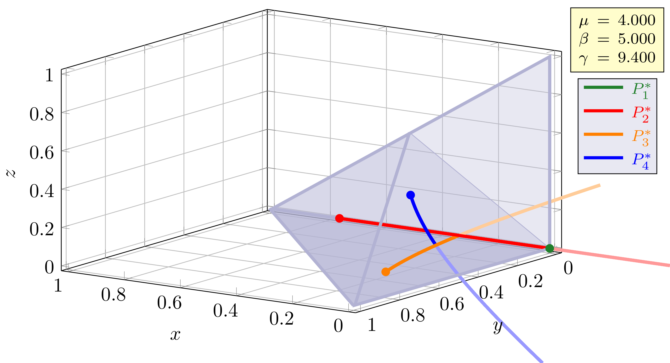
The dynamical system defined by (1) has the following four (biologically meaningful) fixed points in the domain $\mathcal{E}$ (see Figure 4):

	$\displaystyle P_{1}^{*}$	$\displaystyle=(0,0,0),$
	$\displaystyle P_{2}^{*}$	$\displaystyle=\left(\frac{\mu-1}{\mu},0,0\right),$
	$\displaystyle P_{3}^{*}$	$\displaystyle=\left(\frac{1}{\beta},1-\frac{1}{\mu}-\frac{1}{\beta},0\right),$
	$\displaystyle P_{4}^{*}$	$\displaystyle=\left(\frac{1}{2}\left(1-\mu^{-1}+\beta^{-1}-\gamma^{-1}\right),\frac{1}{\gamma},\frac{1}{2}\left(1-\mu^{-1}-\beta^{-1}-\gamma^{-1}\right)\right).$

Notice that the system admits a fifth fixed point $P_{5}^{*}=\left(0,\tfrac{1}{\gamma},-\tfrac{1}{\beta}\right),$ which is not biologically meaningful since it has a negative coordinate (recall that $\beta>0$ ), and thus it will not be taken into account in this study.

The fixed points $P_{1}^{*}$ , $P_{2}^{*}$ , and $P_{3}^{*}$ are boundary equilibria, while $P_{4}^{*}$ is a boundary equilibrium if $\mu^{-1}+\beta^{-1}+\gamma^{-1}=1$ and interior otherwise. The fixed point $P_{1}^{*}$ is the origin, representing the extinction of all the species. $P_{2}^{*}$ is a boundary fixed point, with absence of the two predator species. The point $P_{3}^{*}$ is the boundary fixed point in the absence of the top-level predator $z=0$ , while the point $P_{4}^{*}$ , when it is located in the interior of $\mathcal{E}$ , corresponds to a coexistence equilibrium.

The next lemma gives necessary and sufficient conditions in order that the fixed points $P_{1}^{*},P_{2}^{*},P_{3}^{*}$ , and $P_{4}^{*}$ are biologically meaningful (belong to the domain $\mathbb{U}$ and, hence, to $\mathcal{E}$ — see, for instance, Figure 4 and Movie-2.avi in the Supplementary Material; see also the right part of Figure 5).

Lemma 3.

The following statements hold for every parameters’ choice $(\mu,\beta,\gamma)\in\mathsf{Q}$ :

$P_{1}^{*}:$

The fixed point $P_{1}^{*}$ belongs to $\mathcal{E}.$
$P_{2}^{*}:$

The fixed point $P_{2}^{*}$ belongs to $\mathcal{E}$ if and only if $\mu\geq 1.$ Moreover, $P_{2}^{*}=P_{1}^{*}$ if and only if $\mu=1.$
$P_{3}^{*}:$

The fixed point $P_{3}^{*}$ belongs to $\mathcal{E}$ if and only if $\mu\geq\tfrac{\beta}{\beta-1}\geq\tfrac{5}{4}$ (which is equivalent to $\tfrac{1}{\mu}+\tfrac{1}{\beta}\leq 1$ ). Moreover, $P_{3}^{*}=P_{2}^{*}$ if and only if $\mu=\tfrac{\beta}{\beta-1}.$
$P_{4}^{*}:$

The fixed point $P_{4}^{*}$ belongs to $\mathcal{E}$ if and only if $\mu^{-1}+\beta^{-1}+\gamma^{-1}\leq 1$ (which is equivalent to $\mu\geq\tfrac{\beta\gamma}{(\beta-1)\gamma-\beta}$ ). Moreover, $P_{4}^{*}=P_{3}^{*}$ if and only if $\mu^{-1}+\beta^{-1}+\gamma^{-1}=1.$

Proof.

The statements concerning $P_{1}^{*}$ and $P_{2}^{*}$ follow straightforwardly from their formulae (see also Figure 4) since, for $\mu\geq 1,$ $\frac{\mu-1}{\mu}\in\left[0,\tfrac{3}{4}\right].$

For the fixed point $P_{3}^{*}$ when $\tfrac{1}{\mu}+\tfrac{1}{\beta}\leq 1$ we have $0<\frac{1}{\beta},$ $0\leq 1-\frac{1}{\mu}-\frac{1}{\beta},$ and $\frac{1}{\beta}+\left(1-\frac{1}{\mu}-\frac{1}{\beta}\right)=1-\frac{1}{\mu}<1.$ So,

P_{3}^{*}\in\{(x,y,0)\in\mathbb{R}^{3}\,\colon x,y\geq 0\text{ and }x+y\leq 1\}\subset\{(x,y,0)\in\mathcal{E}\}\subset\mathcal{E}.

Moreover, when $\tfrac{1}{\mu}+\tfrac{1}{\beta}=1$ we have

P_{3}^{*}=\left(\frac{1}{\beta},1-\frac{1}{\mu}-\frac{1}{\beta},0\right)=\left(1-\frac{1}{\mu},0,0\right)=P_{2}^{*}.

For the fixed point $P_{4}^{*}=\left(\tfrac{1}{2}\left(1-\mu^{-1}+\beta^{-1}-\gamma^{-1}\right),\tfrac{1}{\gamma},\tfrac{1}{2}\left(1-\mu^{-1}-\beta^{-1}-\gamma^{-1}\right)\right)$ when $\mu^{-1}+\beta^{-1}+\gamma^{-1}\leq 1$ we have

	$\displaystyle 0$	$\displaystyle<\frac{1}{\gamma},$
	$\displaystyle 0$	$\displaystyle\leq\frac{1}{2}\left(1-\mu^{-1}-\beta^{-1}-\gamma^{-1}\right),$
	$\displaystyle 0$	$\displaystyle<\beta^{-1}\leq\frac{1}{2}\left(1-\mu^{-1}+\beta^{-1}-\gamma^{-1}\right),\text{ and}$
		$\displaystyle\phantom{<}\frac{1}{2}\left(1-\mu^{-1}+\beta^{-1}-\gamma^{-1}\right)+\frac{1}{\gamma}+\frac{1}{2}\left(1-\mu^{-1}-\beta^{-1}-\gamma^{-1}\right)=1-\frac{1}{\mu}<1.$

So,

P_{4}^{*}\in\{(x,y,z)\in\mathbb{U}\,\colon y>0\text{ and }x\geq z\}\subset\mathcal{E}.

Moreover, when $\mu^{-1}+\beta^{-1}+\gamma^{-1}=1$ ( $1-\mu^{-1}-\beta^{-1}-\gamma^{-1}=0$ ) we have

		$\displaystyle\gamma^{-1}=1-\mu^{-1}-\beta^{-1},\text{ and}$
		$\displaystyle 1-\mu^{-1}+\beta^{-1}-\gamma^{-1}=1-\mu^{-1}-\beta^{-1}-\gamma^{-1}+2\beta^{-1}=2\beta^{-1}.$

So,

P_{4}^{*}=\left(\frac{1}{2}\left(1-\mu^{-1}+\beta^{-1}-\gamma^{-1}\right),\frac{1}{\gamma},\frac{1}{2}\left(1-\mu^{-1}-\beta^{-1}-\gamma^{-1}\right)\right)=\\ \left(\beta^{-1},1-\mu^{-1}-\beta^{-1},0\right)=P_{3}^{*}.

∎

Henceforth, this section will be devoted to the study of the local stability and dynamics around the fixed points $P_{1}^{*},\ldots,P_{4}^{*}$ for parameters moving in $\mathsf{Q}.$ This work is carried out by means of four lemmas (Lemmas 4 to 7). The information provided by them is summarized graphically in Figure 5 and Figure 6.

The study of the stability around the fixed points is based on the computation of the eigenvalues of its Jacobian matrix. In our case, the Jacobian matrix of map (1) at a point $(x,y,z)$ is

J(x,y,z)=\begin{pmatrix}\mu(1-2x-y-z)&-\mu x&-\mu x\\ \beta y&\beta(x-z)&-\beta y\\ 0&\gamma z&\gamma y\end{pmatrix}

and has determinant $\det(J(x,y,z))=\mu\beta\gamma xy(1-2x-2z).$ and has determinant $\det(J(x,y,z))=\mu\beta\gamma xy(1-2x-2z).$

The first one of these lemmas follows from a really simple computation.

Lemma 4.

The point $P_{1}^{*}=(0,0,0)$ is a boundary fixed point of system (1) for any positive $\mu$ , $\beta$ , $\gamma.$ Moreover, $P_{1}^{*}$ is:

•

non-hyperbolic when $\mu=1,$
•

a locally asymptotically stable sink node when $0<\mu<1$ , and
•

a saddle with an unstable manifold of dimension 1, locally tangent to the $x$ -axis, when $\mu>1.$

Proof.

The Jacobian matrix of system (1) at $P_{1}^{*}$ is

J(P_{1}^{*})=\begin{pmatrix}\mu&0&0\\ 0&0&0\\ 0&0&0\end{pmatrix},

which has an eigenvalue $\lambda_{1,1}=\mu$ with eigenvector $(1,0,0),$ and two eigenvalues $\lambda_{1,2}=\lambda_{1,3}=0$ with eigenvectors $(0,1,0)$ and $(0,0,1)$ (see Figure 5). Hereafter we will label the eigenvalues $j$ of a fixed point $P_{i}^{*}$ as $\lambda_{i,j}$ , with $i=1,\dots,4$ and $j=1,\dots,3.$ The assertion of the lemma follows from the Hartman-Grobman Theorem. ∎

Lemma 5.

The point $P_{2}^{*}=\left(1-\mu^{-1},0,0\right)$ is a boundary fixed point of the system (1) for all parameters such that $\mu^{-1}\leq 1.$ In particular, for all of the values of the parameters in $\mathsf{Q}$ , the fixed point $P_{2}^{*}$ is non-hyperbolic if and only if:

•

$\mu=1,$ that is, when $P_{2}^{*}=P_{1}^{*}$ ;
•

$\mu=\tfrac{\beta}{\beta-1}$ , that is, when $P_{2}^{*}=P_{3}^{*}$ ;
•

$\mu=3.$

The region of the parameter’s cuboid where $P_{2}^{*}$ is hyperbolic is divided into the following three layers:

$1<\mu<\tfrac{\beta}{\beta-1}$ :

$P_{2}^{*}$ is a locally asymptotically stable sink node, meaning that the two predator species go to extinction.
$\tfrac{\beta}{\beta-1}<\mu<3$ :

$P_{2}^{*}$ is a saddle with an unstable manifold of dimension 1 locally tangent to the $x$ -axis.
$3<\mu\leq 4$ :

$P_{2}^{*}$ is a saddle with an unstable manifold of dimension 2 locally tangent to the plane generated by the vectors $(1,0,0)$ and $\left(1,\tfrac{2-\mu}{\mu-1}-\tfrac{\beta}{\mu},0\right).$

From Lemma 4 it is clear that the fixed points $P_{1,2}^{*}$ and $P_{2,3}^{*}$ undergo a transcritical bifurcation at $\mu=1$ and $\mu=\tfrac{\beta}{\beta-1}$ (in other words, $\mu^{-1}+\beta^{-1}=1$ ), respectively.

Proof.

The Jacobian matrix of system (1) at $P_{2}^{*}$ is

J(P_{2}^{*})=\begin{pmatrix}2-\mu&1-\mu&1-\mu\\ 0&\beta\left(1-\tfrac{1}{\mu}\right)&0\\ 0&0&0\end{pmatrix},

which has:

•

an eigenvalue $\lambda_{2,1}=2-\mu$ with eigenvector $(1,0,0),$
•

an eigenvalue $\lambda_{2,2}=\beta\left(1-\tfrac{1}{\mu}\right)$ with eigenvector $\left(1,\tfrac{2-\mu}{\mu-1}-\tfrac{\beta}{\mu},0\right),$
•

and an eigenvalue $\lambda_{2,3}=0$ with eigenvector $\left(1,0,\tfrac{2-\mu}{\mu-1}\right).$

Moreover, for $1\leq\mu\leq 4$ we have $2-\mu\in[-2,1]$ and $\beta\left(1-\tfrac{1}{\mu}\right)\geq 0.$ Clearly (see Figure 5) one has:

•

$2-\mu=\pm 1$ if and only if $\mu=2\mp 1,$ and $\left\lvert 2-\mu\right\rvert<1$ if and only if $1<\mu<3;$
•

$\beta\left(1-\frac{1}{\mu}\right)=1$ if and only if $\mu=\tfrac{\beta}{\beta-1},$ and $0\leq\beta\left(1-\frac{1}{\mu}\right)<1$ if and only if $1\leq\mu<\tfrac{\beta}{\beta-1};$
•

$1<\tfrac{\beta}{\beta-1}<3$ for every $\beta\in[2.5,5].$

Then the lemma follows from the Hartman-Grobman Theorem. ∎

Lemma 6.

The point $P_{3}^{*}=\left(\beta^{-1},1-\beta^{-1}-\mu^{-1},0\right)$ is a boundary fixed point of the system (1) for all positive parameters such that $\mu^{-1}+\beta^{-1}\leq 1.$ In particular, for all the parameters in $\mathsf{Q}$ , the fixed point $P_{3}^{*}$ is non-hyperbolic if and only if:

•

$\mu=\tfrac{\beta}{\beta-1},$ that is, when $P_{3}^{*}=P_{2}^{*}$ ;
•

$\mu=\tfrac{\beta\gamma}{(\beta-1)\gamma-\beta}$ , that is, when $P_{3}^{*}=P_{4}^{*}$ ;
•

$\mu=\frac{\beta}{\beta-2}.$

The region in $\mathsf{Q}$ where $P_{3}^{*}$ is hyperbolic is divided into the following four layers:

$\tfrac{\beta}{\beta-1}<\mu\leq 2\beta\left(\beta-1-\sqrt{\beta(\beta-2)}\right)$ :

$P_{3}^{*}$ is a locally asymptotically stable sink node. Here preys $x$ and predators $y$ achieve a static equilibrium.
$2\beta\left(\beta-1-\sqrt{\beta(\beta-2)}\right)<\mu<\tfrac{\beta\gamma}{(\beta-1)\gamma-\beta}$ :

$P_{3}^{*}$ is a locally asymptotically stable spiral-node sink. Here preys $x$ and predators $y$ achieve also a static equilibrium, reached via damped oscillations.
$\tfrac{\beta\gamma}{(\beta-1)\gamma-\beta}<\mu<\min\left\{4,\frac{\beta}{\beta-2}\right\}$ :

$P_{3}^{*}$ is an unstable spiral-sink node-source.
$\min\left\{4,\frac{\beta}{\beta-2}\right\}<\mu\leq 4$ :

$P_{3}^{*}$ is an unstable spiral-node source.

From the previous calculations one has that the fixed points $P_{2,3}^{*}$ undergo a transcritical bifurcation at $\mu=\tfrac{\beta}{\beta-1}$ (see also Lemma 5) and $\mu=\tfrac{\beta\gamma}{(\beta-1)\gamma-\beta}$ , respectively¹¹ 1 In terms of inverses of the parameters, these identities read $\mu^{-1}+\beta^{-1}=1$ and $\mu^{-1}+\beta^{-1}+\gamma^{-1}=1.$ .

Proof of Lemma 6.

The Jacobian matrix of system (1) at $P_{3}^{*}$ is

J(P_{3}^{*})=\begin{pmatrix}1-\tfrac{\mu}{\beta}&-\tfrac{\mu}{\beta}&-\tfrac{\mu}{\beta}\\ \beta\left(1-\tfrac{1}{\mu}\right)-1&1&\beta\left(\tfrac{1}{\mu}-1\right)+1\\ 0&0&\gamma\left(1-\tfrac{1}{\beta}-\tfrac{1}{\mu}\right)\end{pmatrix},

and has eigenvalues

	$\displaystyle\lambda_{3,1}$	$\displaystyle=\gamma\left(1-\tfrac{1}{\beta}-\tfrac{1}{\mu}\right),\text{ and}$
	$\displaystyle\lambda_{3,2},\lambda_{3,3}$	$\displaystyle=1-\frac{\mu}{2\beta}\pm\frac{\sqrt{\left(\beta+\tfrac{\mu}{2}\right)^{2}-\beta^{2}\mu}}{\beta}.$

For $\tfrac{\beta}{\beta-1}\leq\mu\leq 4$ we have $\gamma\left(1-\tfrac{1}{\beta}-\tfrac{1}{\mu}\right)\geq 0$ and $\gamma\left(1-\tfrac{1}{\beta}-\tfrac{1}{\mu}\right)=1$ if and only if $\mu=\tfrac{\beta\gamma}{(\beta-1)\gamma-\beta}$ (see Figure 5). On the other hand, $\left(\beta+\tfrac{\mu}{2}\right)^{2}-\beta^{2}\mu=0$ if and only if $\mu=2\beta\left(\beta-1\pm\sqrt{\beta(\beta-2)}\right).$

Now let us study the relation between $\tfrac{\beta}{\beta-1},$ $2\beta\left(\beta-1\pm\sqrt{\beta(\beta-2)}\right),$ $\tfrac{\beta\gamma}{(\beta-1)\gamma-\beta}$ and $\frac{\beta}{\beta-2}.$ First we observe that, since $\beta\geq 2.5,$

2\beta\left(\beta-1+\sqrt{\beta(\beta-2)}\right)\geq 5(1.5+\sqrt{1.25})>13>4\geq\mu.

Consequently, we simultaneously have $\left(\beta+\tfrac{\mu}{2}\right)^{2}-\beta^{2}\mu=0$ and $\mu\leq 4$ if and only if $\mu=2\beta\left(\beta-1-\sqrt{\beta(\beta-2)}\right).$

Second, since $\beta(\beta-2)=(\beta-1)^{2}-1,$ it follows that

\beta(\beta-2)<(\beta-1)^{2}-1+\frac{1}{4(\beta-1)^{2}}=\left((\beta-1)-\tfrac{1}{2(\beta-1)}\right)^{2}.

Moreover, $\beta(\beta-2)>0$ and $(\beta-1)-\tfrac{1}{2(\beta-1)}>0$ (which follows from the inequality $2(\beta-1)^{2}>1$ ). So, the above inequality is equivalent to

\sqrt{\beta(\beta-2)}<(\beta-1)-\frac{1}{2(\beta-1)}\qquad\Longleftrightarrow\qquad\frac{1}{2(\beta-1)}<(\beta-1)-\sqrt{\beta(\beta-2)}

which, in turn, is equivalent to

\frac{\beta}{\beta-1}<2\beta\left(\beta-1-\sqrt{\beta(\beta-2)}\right).

Third, we will show that

(3)

2\beta\left(\beta-1-\sqrt{\beta(\beta-2)}\right)<\frac{\beta\gamma}{(\beta-1)\gamma-\beta}.

To this end observe that

(4)

\frac{\partial}{\partial\gamma}\frac{\gamma}{(\beta-1)\gamma-\beta}=-\frac{\beta}{((\beta-1)\gamma-\beta)^{2}}<0.

Hence, by replacing $9.4$ by $\tfrac{47}{5},$

\frac{47}{42\beta-47}=\frac{\tfrac{47}{5}}{\tfrac{47(\beta-1)}{5}-\beta}\leq\frac{\gamma}{(\beta-1)\gamma-\beta}.

So, to prove (3), it is enough to show that

\beta-1-\sqrt{\beta(\beta-2)}<\frac{47}{2(42\beta-47)}\leq\frac{1}{2\beta}\frac{\beta\gamma}{(\beta-1)\gamma-\beta}.

This inequality is equivalent to

\frac{84\beta^{2}-178\beta+47}{84\beta-94}=\beta-1-\frac{47}{84\beta-94}<\sqrt{\beta(\beta-2)}.

Since $\beta\geq 2.5,$ $\tfrac{84\beta^{2}-178\beta+47}{84\beta-94}$ is positive and thus, it is enough to prove that

\frac{(84\beta^{2}-178\beta+47)^{2}}{(84\beta-94)^{2}}<\beta(\beta-2),

which is equivalent to

0<\beta(\beta-2)(84\beta-94)^{2}-(84\beta^{2}-178\beta+47)^{2}=840\beta^{2}-940\beta-2209.

This last polynomial is positive for every

\beta>\frac{47\sqrt{235}+235}{420}\approx 2.27499\cdots\;.

This ends the proof of (3). On the other hand, since $\gamma\geq 5\geq\beta,$ we have $-\beta\gamma\leq-\beta^{2}$ which is equivalent to

\beta\gamma(\beta-2)=\beta^{2}\gamma-2\beta\gamma\leq\beta^{2}\gamma-\beta\gamma-\beta^{2}=\beta((\beta-1)\gamma-\beta),

and this last inequality is equivalent to

\frac{\beta\gamma}{(\beta-1)\gamma-\beta}\leq\frac{\beta}{\beta-2}

(with equality only when $\gamma=5=\beta$ ). Thus, summarizing, we have seen:

(5)

1<\frac{\beta}{\beta-1}<2\beta\left(\beta-1-\sqrt{\beta(\beta-2)}\right)<\frac{\beta\gamma}{(\beta-1)\gamma-\beta}\leq\frac{\beta}{\beta-2}

and the last inequality is an equality only when $\gamma=5=\beta.$

Next we study the modulus of the eigenvalues to determine the local stability of $P_{3}^{*}.$ First observe (see Figure 5) that $\left\lvert\lambda_{3,1}\right\rvert=\left\lvert\gamma\left(1-\tfrac{1}{\beta}-\tfrac{1}{\mu}\right)\right\rvert<1$ if and only if $\tfrac{\beta}{\beta-1}<\mu<\tfrac{\beta\gamma}{(\beta-1)\gamma-\beta}.$ On the other hand, on $\tfrac{\beta}{\beta-1}<\mu\leq 2\beta\left(\beta-1-\sqrt{\beta(\beta-2)}\right),$ the discriminant $\left(\beta+\tfrac{\mu}{2}\right)^{2}-\beta^{2}\mu$ is non-negative and the eigenvalues $\lambda_{3,2}$ and $\lambda_{3,3}$ are real. Moreover, $\beta>2$ is equivalent to $-\beta\mu>\beta\mu-\beta^{2}\mu$ and this to

\left(\beta-\tfrac{\mu}{2}\right)^{2}>\left(\beta+\tfrac{\mu}{2}\right)^{2}-\beta^{2}\mu\quad\Leftrightarrow\quad\beta-\frac{\mu}{2}>\sqrt{\left(\beta+\tfrac{\mu}{2}\right)^{2}-\beta^{2}\mu}

(observe that $\beta-\tfrac{\mu}{2}>0$ because $\beta>2$ and $\mu\leq 4,$ and recall that $\left(\beta+\tfrac{\mu}{2}\right)^{2}-\beta^{2}\mu$ is non-negative in the selected region). The last inequality above is equivalent to

1-\frac{\mu}{2\beta}>\frac{\sqrt{\left(\beta+\tfrac{\mu}{2}\right)^{2}-\beta^{2}\mu}}{\beta}\quad\Leftrightarrow\quad 0<1-\frac{\mu}{2\beta}-\frac{\sqrt{\left(\beta+\tfrac{\mu}{2}\right)^{2}-\beta^{2}\mu}}{\beta}=\lambda_{3,3}.

On the other hand, the following equivalent expressions hold:

	$\displaystyle\frac{\beta}{\beta-1}<\mu\Leftrightarrow\beta^{2}<\mu\beta(\beta-1)\Leftrightarrow\left(\beta+\tfrac{\mu}{2}\right)^{2}-\beta^{2}\mu=\beta^{2}+\frac{\mu^{2}}{4}+\mu\beta-\mu\beta^{2}<\frac{\mu^{2}}{4}$
	$\displaystyle\frac{\sqrt{\left(\beta+\tfrac{\mu}{2}\right)^{2}-\beta^{2}\mu}}{\beta}<\frac{\mu}{2\beta}\Leftrightarrow\lambda_{3,2}=1-\frac{\mu}{2\beta}+\frac{\sqrt{\left(\beta+\tfrac{\mu}{2}\right)^{2}-\beta^{2}\mu}}{\beta}<1.$

Summarizing, when $\tfrac{\beta}{\beta-1}<\mu\leq 2\beta\left(\beta-1-\sqrt{\beta(\beta-2)}\right)$ we have

0<\lambda_{3,3}=1-\frac{\mu}{2\beta}-\frac{\sqrt{\left(\beta+\tfrac{\mu}{2}\right)^{2}-\beta^{2}\mu}}{\beta}\leq 1-\frac{\mu}{2\beta}+\frac{\sqrt{\left(\beta+\tfrac{\mu}{2}\right)^{2}-\beta^{2}\mu}}{\beta}=\lambda_{3,2}<1.

Consequently, $P_{3}^{*}$ is a locally asymptotically stable sink node by (5), meaning that top predators ( $z$ ) go to extinction and the other two species persist.

Now we consider the region $2\beta\left(\beta-1-\sqrt{\beta(\beta-2)}\right)<\mu\leq 4.$ In this case the discriminant $\left(\beta+\tfrac{\mu}{2}\right)^{2}-\beta^{2}\mu$ is negative and the eigenvalues $\lambda_{3,2}$ and $\lambda_{3,3}$ are complex conjugate with modulus

\sqrt{\left(1-\tfrac{\mu}{2\beta}\right)^{2}+\frac{\beta^{2}\mu-\left(\beta+\tfrac{\mu}{2}\right)^{2}}{\beta^{2}}}=\sqrt{\frac{\mu(\beta-2)}{\beta}}.

Clearly

\left\lvert\sqrt{\frac{\mu(\beta-2)}{\beta}}\right\rvert<1\quad\Leftrightarrow\quad 2\beta\left(\beta-1-\sqrt{\beta(\beta-2)}\right)\leq\mu\leq\min\left\{4,\frac{\beta}{\beta-2}\right\}

(with equality only when $\gamma=5=\beta$ ). Then the lemma follows from the Hartman-Grobman Theorem. ∎

Lemma 7.

The point $P_{4}^{*}=\left(\rho,\gamma^{-1},\rho-\beta^{-1}\right)$ with $\rho=\tfrac{1}{2}\left(1+\beta^{-1}-\gamma^{-1}-\mu^{-1}\right)$ is a fixed point of the system (1) for all positive parameters satisfying that $\mu^{-1}+\beta^{-1}+\gamma^{-1}\leq 1.$ Moreover, for all the parameters in $\mathsf{Q}$ , there exists a function $\psi_{4}\colon[2.5,5]\times[5,9.4]\longrightarrow\left[\tfrac{\beta\gamma}{(\beta-1)\gamma-\beta},4\right)$ (whose graph $\Sigma_{4}$ is drawn in redish colour in Figure 5) such that $P_{4}^{*}$ is non-hyperbolic if and only if:

•

$\mu=\tfrac{\beta\gamma}{(\beta-1)\gamma-\beta}$ , that is, when $P_{4}^{*}=P_{3}^{*}$ ;
•

$\mu=\psi_{4}(\beta,\gamma).$

Furthermore, the region of the parameter’s cuboid where $P_{4}^{*}$ is hyperbolic is divided into the following two layers:

$\tfrac{\beta\gamma}{(\beta-1)\gamma-\beta}<\mu<\psi_{4}(\beta,\gamma)$ :

$P_{4}^{*}$ is a locally asymptotically stable sink of spiral-node type. Within this first layer the three species achieve a static coexistence equilibrium with an oscillatory transient.
$\psi_{4}(\beta,\gamma)<\mu\leq 4$ :

$P_{4}^{*}$ is an unstable spiral-source node-sink.

Proof.

The Jacobian matrix of system (1) at $P_{4}^{*}$ is

J(P_{4}^{*})=\begin{pmatrix}1-\mu\rho&-\mu\rho&-\mu\rho\\ \tfrac{\beta}{\gamma}&1&-\tfrac{\beta}{\gamma}\\ 0&\gamma\left(\rho-\tfrac{1}{\beta}\right)&1\end{pmatrix}\;.

The matrix $J(P_{4}^{*})$ has eigenvalues

	$\displaystyle\lambda_{4,1}$	$\displaystyle:=1-\frac{\mu\rho}{3}+\frac{\sqrt[3]{\alpha}}{3\sqrt[3]{2}\sqrt{\gamma}}+\frac{\sqrt[3]{2}\left(\mu^{2}\rho^{2}\gamma-3\beta(\mu+\gamma)\rho+3\gamma\right)}{3\sqrt{\gamma}\sqrt[3]{\alpha}},$
	$\displaystyle\lambda_{4,2},\lambda_{4,3}$	$\displaystyle:=1-\frac{\mu\rho}{3}-\frac{\sqrt[3]{\alpha}}{3\sqrt[3]{16}\sqrt{\gamma}}(1\mp\sqrt{3}i)-\frac{\mu^{2}\rho^{2}\gamma-3\beta(\mu+\gamma)\rho+3\gamma}{3\sqrt[3]{4}\sqrt{\gamma}\sqrt[3]{\alpha}}\left(1\pm\sqrt{3}i\right),$

where

	$\displaystyle\alpha=$	$\displaystyle\ -2\gamma^{3/2}\rho^{3}\mu^{3}-45\gamma^{3/2}\beta\mu\rho^{2}+9\mu^{2}\rho^{2}\beta\sqrt{\gamma}+45\gamma^{3/2}\rho\mu+\sqrt{27\widetilde{\alpha}},\text{ and}$
	$\displaystyle\widetilde{\alpha}:=$	$\displaystyle\ 8(\rho\,\beta-1)\left(\mu^{4}\rho^{4}+\frac{71(\rho\beta-1)\rho^{2}\mu^{2}}{8}+\frac{(\beta\rho-1)^{2}}{2}\right)\gamma^{3}$
		$\displaystyle\ -38(\rho\beta-1)\left(\mu^{2}\rho^{2}-\frac{6(\rho\beta-1)}{19}\right)\rho\beta\mu\gamma^{2}$
		$\displaystyle\ -\mu^{2}\rho^{2}\beta^{2}\left(\mu^{2}\rho^{2}-12(\rho\beta-1)\right)\gamma+4\beta^{3}\mu^{3}\rho^{3}.$

When $\mu=\tfrac{\beta\gamma}{(\beta-1)\gamma-\beta}$ we clearly have

J(P_{4}^{*})=\begin{pmatrix}1-\mu\rho&-\mu\rho&-\mu\rho\\ \tfrac{\beta}{\gamma}&1&-\tfrac{\beta}{\gamma}\\ 0&0&1\end{pmatrix}

and

\begin{pmatrix}1-\mu\rho&-\mu\rho&-\mu\rho\\ \tfrac{\beta}{\gamma}&1&-\tfrac{\beta}{\gamma}\\ 0&0&1\end{pmatrix}\begin{pmatrix}\phantom{+}1\\ -2\\ \phantom{+}1\end{pmatrix}=\begin{pmatrix}\phantom{+}1\\ -2\\ \phantom{+}1\end{pmatrix}\;.

Thus, for every $(\beta,\gamma)\in[2.5,5]\times[5,9.4],$ $\lambda_{4,1}=1$ when $\mu=\tfrac{\beta\gamma}{(\beta-1)\gamma-\beta}.$ Moreover, it can be seen numerically that for every $(\beta,\gamma)\in[2.5,5]\times[5,9.4],$ $\lambda_{4,1}$ is a strictly decreasing function of $\mu$ such that $\lambda_{4,1}>-1$ when $\mu=4.$ So, $\lambda_{4,1}$ only breaks the hyperbolicity of $P^{*}_{4}$ in the surface $\mu=\tfrac{\beta\gamma}{(\beta-1)\gamma-\beta}$ and $\left\lvert\lambda_{4,1}\right\rvert<1$ in the region

(\beta,\gamma,\mu)\in[2.5,5]\times[5,9.4]\times\left(\tfrac{\beta\gamma}{(\beta-1)\gamma-\beta},4\right].

Next we need to describe the behaviour of $\left\lvert\lambda_{4,2}\right\rvert=\left\lvert\lambda_{4,3}\right\rvert$ as a function of $\mu.$ The following statements have been observed numerically:

(i)

$\left\lvert\lambda_{4,2}\right\rvert=\left\lvert\lambda_{4,3}\right\rvert<1$ for every

(\beta,\gamma,\mu)\in[2.5,5]\times[5,9.4]\times\left\{\tfrac{\beta\gamma}{(\beta-1)\gamma-\beta}\right\}\setminus\left\{\left(5,5,\tfrac{\beta\gamma}{(\beta-1)\gamma-\beta}\right)\right\}

and $\left\lvert\lambda_{4,2}\right\rvert=\left\lvert\lambda_{4,3}\right\rvert=1$ at the point $(\beta,\gamma,\mu)=\left(5,5,\tfrac{\beta\gamma}{(\beta-1)\gamma-\beta}\right).$

(ii)

$\left\lvert\lambda_{4,2}\right\rvert=\left\lvert\lambda_{4,3}\right\rvert>1$ for every $(\beta,\gamma,\mu)\in[2.5,5]\times[5,9.4]\times\{4\}.$

(iii.1)

There exists a Non-Monotonic (NM) region $\textsf{NM}_{4}\subset[2.5,2.59597\cdots]\times[5,6.49712\cdots]$ such that for every $(\beta,\gamma)\in\textsf{NM}_{4}$ there exists a value $\mu^{*}(\beta,\gamma)\in\left(\tfrac{\beta\gamma}{(\beta-1)\gamma-\beta},4\right)$ with the property that $\left\lvert\lambda_{4,2}\right\rvert=\left\lvert\lambda_{4,3}\right\rvert$ is a strictly decreasing function of the parameter $\mu\in\left[\tfrac{\beta\gamma}{(\beta-1)\gamma-\beta},\mu^{*}(\beta,\gamma)\right],$ and a strictly increasing function of $\mu$ for every value of $\mu\in\left[\mu^{*}(\beta,\gamma),4\right].$ In particular, from (i) it follows that $\left\lvert\lambda_{4,2}\right\rvert=\left\lvert\lambda_{4,3}\right\rvert<1$ holds for every point $(\beta,\gamma,\mu)\in\textsf{NM}_{4}\times\left[\tfrac{\beta\gamma}{(\beta-1)\gamma-\beta},\mu^{*}(\beta,\gamma)\right].$ Consequently, for every $(\beta,\gamma)\in\textsf{NM}_{4},$ there exists a unique value of the parameter $\mu=\psi_{4}(\beta,\gamma)>\mu^{*}(\beta,\gamma)$ such that $\left\lvert\lambda_{4,2}\right\rvert=\left\lvert\lambda_{4,3}\right\rvert=1$ at the point $(\beta,\gamma,\psi_{4}(\beta,\gamma)).$ The region $\textsf{NM}_{4},$ as shown in the picture at the side, is delimited by the axes $\beta=2.5,$ $\gamma=5$ and, approximately, by the curve $\gamma\approx 19.6981\beta^{2}-115.98\beta+173.334.$
(iii.2)

For every $(\beta,\gamma)\in\left([2.5,5]\times[5,9.4]\right)\setminus\textsf{NM}_{4},$ $\left\lvert\lambda_{4,2}\right\rvert=\left\lvert\lambda_{4,3}\right\rvert$ is a strictly increasing function of $\mu.$ In particular, from (i) it follows that there exists a unique value of $\mu=\psi_{4}(\beta,\gamma)>\tfrac{\beta\gamma}{(\beta-1)\gamma-\beta}$ such that $\left\lvert\lambda_{4,2}\right\rvert=\left\lvert\lambda_{4,3}\right\rvert=1$ at the point $(\beta,\gamma,\psi_{4}(\beta,\gamma)).$

Then the lemma follows from the Hartman-Grobman Theorem. ∎

4. Local bifurcations: Three dimensional bifurcation diagram

Due to the mathematical structure of the map (1) and to the number of parameters one can provide analytical information on local dynamics within different regions of the chosen parameter space. That is, to build a three-dimensional bifurcation diagram displaying the parametric regions involved in the local dynamics of the fixed points investigated above. These analyses also provide some clues on the expected global dynamics, that will be addressed numerically in Section 6. To understand the local dynamical picture, the next lemma relates all the surfaces that play a role in defining the local structural stability zones in the previous four lemmas. It justifies the relative positions of these surfaces, shown in Figure 5.

We define

\mathsf{H}_{4}:=\left\{(\beta,\gamma)\colon\psi_{4}(\beta,\gamma)\geq 3\right\}.

Lemma 8.

The relations between the surfaces defined in Lemmas 4–7 are the following:

(i)

For every $(\beta,\gamma)\in[2.5,5]\times[5,9.4],$

$1<\frac{\beta}{\beta-1}<2\beta\left(\beta-1-\sqrt{\beta(\beta-2)}\right)<\frac{\beta\gamma}{(\beta-1)\gamma-\beta}.$

$\mathsf{H}_{4}$ is the region contained in $[2.5,2.769\cdots]\times[5,6.068\cdots]$ and delimited by the axes $\beta=2.5$ and $\gamma=5,$ and the curve

\gamma\approx 2.13725\beta^{2}-15.2038\beta+30.7162.

(ii)

For every $(\beta,\gamma)\in\left(\left[2.5,\tfrac{8}{3}\right]\times[5,9.4]\right)\cap\mathsf{H}_{4},$

$\frac{\beta\gamma}{(\beta-1)\gamma-\beta}<3\leq\psi_{4}(\beta,\gamma)<4\leq\frac{\beta}{\beta-2}.$

On the other hand, for every $(\beta,\gamma)\in\left(\left[2.5,\tfrac{8}{3}\right]\times[5,9.4]\right)\setminus\mathsf{H}_{4},$

$\frac{\beta\gamma}{(\beta-1)\gamma-\beta}<\psi_{4}(\beta,\gamma)<3<4\leq\frac{\beta}{\beta-2}.$
(iii)

For every $(\beta,\gamma)\in\left(\left(\tfrac{8}{3},3\right)\times[5,9.4]\right)\cap\mathsf{H}_{4},$

$\frac{\beta\gamma}{(\beta-1)\gamma-\beta}<3\leq\psi_{4}(\beta,\gamma)<\frac{\beta}{\beta-2}<4$

For every $(\beta,\gamma)\in\left(\left(\tfrac{8}{3},3\right)\times[5,9.4]\right)\setminus\mathsf{H}_{4},$

$\frac{\beta\gamma}{(\beta-1)\gamma-\beta}<\psi_{4}(\beta,\gamma)<3<\frac{\beta}{\beta-2}<4.$
(iv)

For every $(\beta,\gamma)\in\{3\}\times[5,9.4],$

$\frac{\beta\gamma}{(\beta-1)\gamma-\beta}<\psi_{4}(\beta,\gamma)<3=\frac{\beta}{\beta-2}.$
(v)

For every $(\beta,\gamma)\in(3,5]\times[5,9.4],$

$\frac{\beta\gamma}{(\beta-1)\gamma-\beta}\leq\psi_{4}(\beta,\gamma)\leq\frac{\beta}{\beta-2}<3.$

Moreover, all the above inequalities are strict except in the point $(\beta,\gamma)=(5,5)$ where $\frac{\beta\gamma}{(\beta-1)\gamma-\beta}=\psi_{4}(\beta,\gamma)=\frac{\beta}{\beta-2}.$

Proof.

Statement (i) follows from Equation (5) and the fact that $\mathsf{H}_{4}$ is the region delimited by the axes $\beta=2.5$ and $\gamma=5,$ and the curve

\gamma\approx 2.13725\beta^{2}-15.2038\beta+30.7162

can be checked numerically.

On the other hand, observe that for every $\gamma\in[5,9.4]$ we have

\begin{cases}\frac{\beta}{\beta-2}\geq 4&\text{for $\beta\in\left[2.5,\tfrac{8}{3}\right]$,}\\ 4>\frac{\beta}{\beta-2}>3&\text{for $\beta\in\left(\tfrac{8}{3},3\right)$,}\\ \frac{\beta}{\beta-2}=3&\text{for $\beta=\tfrac{8}{3}$,}\\ 3>\frac{\beta}{\beta-2}&\text{for $\beta\in(3,5].$}\end{cases}

Moreover, $7\beta>15$ is equivalent to $12\beta-15>5\beta,$ and Equation (4) implies

3>\frac{5\beta}{4\beta-5}=\beta\frac{5}{5(\beta-1)-\beta}\geq\beta\frac{\gamma}{(\beta-1)\gamma-\beta}.

So, Statements (ii–v) follow from these observations, Equation (5) and by checking numerically the various relations of $\psi_{4}(\beta,\gamma)$ with $\mu=\frac{\beta\gamma}{(\beta-1)\gamma-\beta},$ $\mu=3,$ and $\mu=\frac{\beta}{\beta-2}$ for the different regions considered in Statements (ii–v). ∎

The detailed description of the local dynamics in the zones of Figure 5 (see also Figure 6) is given by the following (see Lemmas 4–8):

Theorem 9.

The following statements hold:

Zone A:

$(\beta,\gamma,\mu)\in[2.5,5]\times[5,9.4]\times(0,1).$
In this layer the system has $P_{1}^{*}=(0,0,0)$ as a unique fixed point. This fixed point is a locally asymptotically stable sink node, meaning that the three species go to extinction. Indeed, it is proved in Theorem 10 that this is a globally asymptotically stable (GAS) point.
Zone B:

$(\beta,\gamma,\mu)\in[2.5,5]\times[5,9.4]\times\left(1,\tfrac{\beta}{\beta-1}\right).$
In this zone the system has exactly two fixed points: the origin $P_{1}^{*}$ and $P_{2}^{*}=\left(1-\tfrac{1}{\mu},0,0\right).$ $P_{1}^{*}$ is a saddle with $\mathrm{dim}\,W^{u}(P_{1}^{*})=1$ locally tangent to the $x$ -axis and $P_{2}^{*}$ is a locally asymptotically stable sink node. Hence, in this zone only preys will survive. Theorem 14 proves that in this zone $P_{2}^{*}$ is a GAS point.

Figure 6. Changes in the existence and local stability of the fixed points tied to the transitions between the zones identified in Figure 5. The tables display, for each fixed point, the stability nature along the thick arrows displayed in the cuboid $\mathsf{Q}.$ The fixed points are classified as follows: asymptotically stable sink (AS); non-spiral saddle with a 1-dimensional $(S_{1})$ and 2-dimensional $(S_{2})$ stable manifold; and spirals (stable in blue; unstable in red), see the legend below the table framed in light blue. Stable and unstable manifolds are displayed with blue and red arrows, respectively. The small violet arrows in the lower table denote transcritical bifurcations, with collision of fixed points and stability changes. The small orange arrows indicate changes in stability without collision of fixed points. Here numerical evidences for supercritical Neimark-Sacker bifurcations have been obtained (indicated with an asterisk).
Zone C:

$(\beta,\gamma,\mu)\in[2.5,5]\times[5,9.4]\times\left(\tfrac{\beta}{\beta-1},2\beta\left(\beta-1-\sqrt{\beta(\beta-2)}\right)\right).$
In this region the system has exactly three fixed points: the origin $P_{1}^{*},$ $P_{2}^{*}$ and $P_{3}^{*}=\left(\beta^{-1},1-\beta^{-1}-\mu^{-1},0\right).$ $P_{1}^{*}$ and $P_{2}^{*}$ are saddles with $\mathrm{dim}\,W^{u}(P_{1}^{*},P_{2}^{*})=1$ and $P_{3}^{*}$ is a locally asymptotically stable sink node. Here top predators can not survive, being the system only composed of preys and the predator species $y.$
Zone D:

$(\beta,\gamma,\mu)\in[2.5,5]\times[5,9.4]\times\left(2\beta\left(\beta-1-\sqrt{\beta(\beta-2)}\right),\tfrac{\beta\gamma}{(\beta-1)\gamma-\beta}\right).$
In this zone the system still has three fixed points: $P_{1}^{*},$ $P_{2}^{*}$ and $P_{3}^{*}.$ $P_{1}^{*}$ and $P_{2}^{*}$ are saddles with $\mathrm{dim}\,W^{u}(P_{1}^{*},P_{2}^{*})=1$ but $P_{3}^{*}$ is a locally asymptotically stable spiral-node sink. In this region the prey and predator $y$ reach a static equilibrium of coexistence achieved via damped oscillations, while the top predator $z$ goes to extinction.
Zone E:

$(\beta,\gamma,\mu)\in[2.5,5]\times[5,9.4]\times\left(\tfrac{\beta\gamma}{(\beta-1)\gamma-\beta},\min\left\{3,\psi_{4}(\beta,\gamma)\right\}\right).$
In this layer the system has exactly four fixed points: the origin $P_{1}^{*},$ $P_{2}^{*},$ $P_{3}^{*}$ and $P_{4}^{*}=\left(\rho,\gamma^{-1},\rho-\beta^{-1}\right).$ $P_{1}^{*}$ and $P_{2}^{*}$ are saddle points with $\mathrm{dim}\,W^{u}(P_{1}^{*},P_{2}^{*})=1,$ the fixed point $P_{3}^{*}$ is an unstable spiral-sink node-source and $P_{4}^{*}$ is a locally asymptotically stable sink of spiral-node type. Under this scenario, the three species achieve a static coexistence state also via damped oscillations.
Zone F:

$(\beta,\gamma,\mu)\in\left(\left([2.5,5]\times[5,9.4]\right)\setminus\mathsf{H}_{4}\right)\times\left(\psi_{4}(\beta,\gamma),\min\left\{3,\frac{\beta}{\beta-2}\right\}\right).$
In this layer the system has exactly four fixed points: the origin $P_{1}^{*},$ $P_{2}^{*},$ $P_{3}^{*}$ and $P_{4}^{*}=\left(\rho,\gamma^{-1},\rho-\beta^{-1}\right).$ The fixed points $P_{1}^{*}$ and $P_{2}^{*}$ are saddles with $\mathrm{dim}\,W^{u}(P_{1}^{*},P_{2}^{*})=1,$ the point $P_{3}^{*}$ is an unstable spiral-sink node-source and $P_{4}^{*}$ is an unstable spiral-source node-sink. Here, due to the unstable nature of all fixed points, fluctuating coexistence of all of the species is found. As we will see in Section 5, this coexistence can be governed by periodic or chaotic fluctuations.
Zone G:

$(\beta,\gamma,\mu)\in(3,5]\times[5,9.4]\times\left(\frac{\beta}{\beta-2},3\right).$
In this zone the system has four fixed points: $P_{1}^{*},$ $P_{2}^{*},$ $P_{3}^{*}$ and $P_{4}^{*}.$ $P_{1}^{*}$ and $P_{2}^{*}$ are a saddles with $\mathrm{dim}\,W^{u}(P_{1}^{*},P_{2}^{*})=1$ , $P_{3}^{*}$ is an unstable spiral-node source and $P_{4}^{*}$ is an unstable spiral-source node-sink. The expected coexistence dynamics here are like those of zone F above.
Zone H:

$(\beta,\gamma,\mu)\in\mathsf{H}_{4}\times\left(3,\psi_{4}(\beta,\gamma)\right).$
In this region the system has four fixed points: $P_{1}^{*},$ $P_{2}^{*},$ $P_{3}^{*}$ and $P_{4}^{*}.$ $P_{1}^{*}$ and $P_{2}^{*}$ are saddles $\mathrm{dim}\,W^{u}(P_{1}^{*},P_{2}^{*})=1,$ $P_{3}^{*}$ is an unstable spiral-sink node-source and $P_{4}^{*}$ is a locally asymptotically stable sink of spiral-node type. The dynamics here are the same as the ones in zone E.
Zone I:

$(\beta,\gamma,\mu)\in(2.5,3)\times[5,9.4]\times\left(\max\left\{3,\psi_{4}(\beta,\gamma)\right\},\min\left\{4,\frac{\beta}{\beta-2}\right\}\right).$
In this zone the system has four fixed points: $P_{1}^{*},$ $P_{2}^{*},$ $P_{3}^{*}$ and $P_{4}^{*}.$ $P_{1}^{*}$ is a saddle with $\mathrm{dim}\,W^{u}(P_{1}^{*})=1$ , $P_{2}^{*}$ is a saddle with $\mathrm{dim}\,W^{u}(P_{2}^{*})=2$ , $P_{3}^{*}$ is an unstable spiral-sink node-source and $P_{4}^{*}$ is an unstable spiral-source node-sink. Here the dynamics can be also governed by coexistence among the three species via oscillations.
Zone J:

$(\beta,\gamma,\mu)\in\left(\tfrac{8}{3},5\right]\times[5,9.4]\times\left(\max\left\{3,\frac{\beta}{\beta-2}\right\},4\right).$
In this zone the system has four fixed points: $P_{1}^{*},$ $P_{2}^{*},$ $P_{3}^{*}$ and $P_{4}^{*}.$ The fixed point $P_{1}^{*}$ is a saddle with $\mathrm{dim}\,W^{u}(P_{1}^{*})=1,$ the point $P_{2}^{*}$ is a saddle with $\mathrm{dim}\,W^{u}(P_{2}^{*})=2$ , $P_{3}^{*}$ is an unstable spiral-node source and $P_{4}^{*}$ is an unstable spiral-source node-sink. Dynamics here can also be governed by all-species fluctuations, either periodic or chaotic.

Figure 6 provides a summary of the changes in the existence and local stability of the fixed points for each one of the zones identified. Also, we provide an animation of the dynamical outcomes tied to crossing the cuboid following the direction of the dashed thick blue arrow represented in Figure 5. Specifically, the file Movie-3.mp4 in the Supplementary Material displays the dynamics along this line for variable $x_{n}$ (as a function of the three running parameters labelled factor), as well as in the phase space $(x,y)$ and $(x,y,z).$

5. Some remarks on global dynamics

In this section we study the global dynamics in Zones A and B from the preceding section.

Theorem 10 (Global dynamics in Zone A).

Assume that $\mu<1$ and let $(x,y,z)$ be a point from $\mathcal{S}.$ Then,

\lim_{n\to\infty}T^{n}(x,y,z)=(0,0,0)=P_{1}^{*}.

In what follows, $\lambda_{\mu}(\sigma):=\mu\sigma(1-\sigma)$ will denote the logistic map.

Proof of Theorem 10.

From Figure 5 (or Lemmata 4–7) it follows that $(0,0,0)$ is the only fixed point of $T$ whenever $\mu<1$ and it is locally asymptotically stable.

We denote $(x_{0},y_{0},z_{0})=(x,y,z)\in\mathcal{S}$ and $(x_{n},y_{n},z_{n})=T^{n}(x,y,z)\in\mathcal{E}$ for every $n\geq 1.$ Assume that there exists $n\geq 0$ such that $y_{n}=0.$ Then, substituting $(x_{n},0,z_{n})$ into Equations (1) it follows that $y_{n+1}=z_{n+1}=0$ and so

T^{n+1}(x,y,z)=(x_{n+1},0,0)\in[0,1]\times\{0\}\times\{0\},

and $T^{n+1+k}(x,y,z)=(\lambda_{\mu}^{k}(x_{n+1}),0,0)$ for every $k\geq 0.$ Since, $\mu<1,$ one gets $\lim_{k\to\infty}\lambda_{\mu}^{k}(\sigma)=0$ for every $\sigma\in[0,1].$ So, the proposition holds in this case.

In the rest of the proof we assume that $y_{n}>0$ for every $n\geq 0.$ We claim that

x_{n}\leq\frac{\mu^{n}}{4}

for every $n\geq 1.$ Let us prove the claim. Since $(x,y,z)\in\mathcal{S}\subset\mathcal{E}$ (Proposition 2) with $y>0$ we have $x\geq z\geq 0$ and $x+y+z\leq 1.$ Thus,

x_{1}=\mu x(1-x-y-z)\leq\mu x(1-x)\leq\frac{\mu}{4},

which proves the case $n=1.$ Assume now that the claim holds for some $n\geq 1$ and prove it for $n+1.$ As before, $(x_{n},y_{n},z_{n})\in\mathcal{E}$ with $y_{n}>0$ implies $x_{n}\geq z_{n}\geq 0$ and $x_{n}+y_{n}+z_{n}\leq 1.$ Hence,

x_{n+1}=\mu x_{n}(1-x_{n}-y_{n}-z_{n})\leq\mu x_{n}\leq\mu\frac{\mu^{n}}{4}=\frac{\mu^{n+1}}{4}.

On the other hand, by using again the assumption that $(x_{n},y_{n},z_{n})\in\mathcal{E}$ with $1\geq y_{n}>0$ for every $n\geq 0,$ and the definition of $T$ in (1), we get that $x_{n}>z_{n}\geq 0$ for every $n\geq 0.$ Moreover, $y_{n+1}=\beta y_{n}(x_{n}-z_{n})\leq\beta y_{n}x_{n}\leq\beta x_{n}.$ Hence, for every $n\geq 0,$

0\leq z_{n}<x_{n}\leq\frac{\mu^{n}}{4}\quad\text{and}\quad 0<y_{n}\leq\beta x_{n-1}\leq\beta\frac{\mu^{n-1}}{4}.

This implies that $\lim_{n\to\infty}(x_{n},y_{n},z_{n})=(0,0,0)$ because $\mu<1.$ ∎

To study the global dynamics in Zone B we need three simple lemmas. The first one is on the logistic map; the second one relates the first coordinate of the image of $T$ with the logistic map; the third one is technical.

Lemma 11 (On the logistic map).

Let $1<\mu<2$ and set $I_{0}:=\bigl[\alpha_{\mu},\widetilde{\alpha}_{\mu}\bigr]$ where $0<\alpha_{\mu}=1-\tfrac{1}{\mu}<\tfrac{1}{2}$ is the stable fixed point of $\lambda_{\mu}$ and $\tfrac{1}{2}<\widetilde{\alpha}_{\mu}<1$ is the unique point such that $\lambda_{\mu}\bigl(\widetilde{\alpha}_{\mu}\bigr)=\alpha_{\mu}.$ Set also $I_{n+1}:=\lambda_{\mu}\bigl(I_{n}\bigr)\subset I_{n}$ for every $n\geq 0.$ Then, for every $\varepsilon>0$ there exists $N\geq 1$ such that $I_{N}\subset\left[\alpha_{\mu},\alpha_{\mu}+\varepsilon\right).$

Proof.

The fact that $0<\alpha_{\mu}=1-\tfrac{1}{\mu}<\tfrac{1}{2}$ is a stable fixed point of $\lambda_{\mu}$ for $1<\mu<2$ is well known. Also, since $\lambda_{\mu}\Bigr\rvert_{\left[\alpha_{\mu},\tfrac{1}{2}\right]}$ is increasing and $1<\mu<2,$ it follows that

\alpha_{\mu}=\lambda_{\mu}\left(\alpha_{\mu}\right)<\dots<\lambda_{\mu}^{n+1}\left(\tfrac{1}{2}\right)<\lambda_{\mu}^{n}\left(\tfrac{1}{2}\right)<\dots<\lambda_{\mu}^{2}\left(\tfrac{1}{2}\right)<\lambda_{\mu}\left(\tfrac{1}{2}\right)<\tfrac{1}{2}.

Therefore,

I_{1}=\lambda_{\mu}\bigl(I_{0}\bigr)=\lambda_{\mu}\left(\left[\alpha_{\mu},\tfrac{1}{2}\right]\right)=\left[\alpha_{\mu},\lambda_{\mu}\left(\tfrac{1}{2}\right)\right]\subset\left[\alpha_{\mu},\tfrac{1}{2}\right]\subset I_{0}

and, for every $n\geq 1,$ one gets

I_{n+1}=\lambda_{\mu}\bigl(I_{n}\bigr)=\left[\alpha_{\mu},\lambda_{\mu}^{n+1}\left(\tfrac{1}{2}\right)\right]\varsubsetneq\left[\alpha_{\mu},\lambda_{\mu}^{n}\left(\tfrac{1}{2}\right)\right]=I_{n}\subset\left[\alpha_{\mu},\tfrac{1}{2}\right].

Then, the lemma follows from the fact that $\lim_{n\to\infty}\lambda_{\mu}^{n}\left(\tfrac{1}{2}\right)=\alpha_{\mu}.$ ∎

Lemma 12.

Let $(x_{0},y_{0},z_{0})\in\mathcal{S}$ and set

(x_{n},y_{n},z_{n}):=T(x_{n-1},y_{n-1},z_{n-1})\in\mathcal{E}

for every $n\geq 1.$ Then, for every $n\geq 1,$

0\leq x_{n}=\lambda_{\mu}(x_{n-1})-\mu x_{n-1}(y_{n-1}+z_{n-1})\leq\lambda_{\mu}(x_{n-1})

and, when $\mu\leq 2,$ it follows that $0\leq x_{n}\leq\lambda^{n}_{\mu}(x_{0})\leq\tfrac{1}{2}.$

Proof.

The first statement is a simple computation:

	$\displaystyle x_{n}$	$\displaystyle=\mu x_{n-1}(1-x_{n-1})-\mu x_{n-1}(y_{n-1}+z_{n-1})$
		$\displaystyle=\lambda_{\mu}(x_{n-1})-\mu x_{n-1}(y_{n-1}+z_{n-1})\leq\lambda_{\mu}(x_{n-1})$

(notice that $\mu,x_{n},x_{n-1},y_{n-1},z_{n-1}\geq 0$ because $(x_{n},y_{n},z_{n})\in\mathcal{E}$ for every $n$ ).

The second statement for $n=1$ follows directly from the first statement and from the fact that $\lambda_{\mu}([0,1])=\lambda_{\mu}\left(\left[0,\tfrac{1}{2}\right]\right)\subset\left[0,\tfrac{1}{2}\right]$ whenever $\mu\leq 2.$

Assume now that the second statement holds for some $n\geq 1.$ Then, from the first statement of the lemma and the fact that $\mu\leq 2$ we have

0\leq x_{n+1}\leq\lambda_{\mu}(x_{n})\leq\lambda_{\mu}\left(\lambda^{n}_{\mu}(x_{0})\right)=\lambda^{n+1}_{\mu}(x_{0})\leq\lambda_{\mu}\left(\tfrac{1}{2}\right)\leq\tfrac{1}{2},

because $\lambda_{\mu}\bigr\rvert_{\left[0,\tfrac{1}{2}\right]}$ is increasing. ∎

The proof of the next technical lemma is a simple exercise.

Lemma 13 (The damped logistic map).

Let $\lambda_{\mu,s}(\sigma):=s\lambda_{\mu}(\sigma)=\mu s\sigma(1-\sigma)$ denote the damped logistic map defined on the interval $[0,1].$ Assume that $1<\mu<2$ and $\tfrac{1}{\mu}<s<1.$ Then the following properties of the damped logistic map hold:

(a)

$\lambda_{\mu,s}(\sigma)<\lambda_{\mu}(\sigma)$ for every $0<\sigma<1.$
(b)

$\lambda_{\mu,s}(0)=0$ and $\lambda_{\mu,s}\Bigr\rvert_{\left[0,\tfrac{1}{2}\right]}$ is strictly increasing.

(c)

$\lambda_{\mu,s}$ has exactly one stable fixed point $\alpha_{\mu,s}:=1-\tfrac{1}{\mu s}$ with derivative

\lambda^{\prime}_{\mu,s}(\alpha_{\mu,s})=\lambda^{\prime}_{\mu,s}(\sigma)\bigr\rvert_{\sigma=\alpha_{\mu,s}}=\mu s(1-2\sigma)\bigr\rvert_{\sigma=\alpha_{\mu,s}}=2-\mu s<1\,.

(d)

For every $\sigma\in\bigl(0,\alpha_{\mu,s}\bigr)$ we have

$\sigma<\lambda_{\mu,s}(\sigma)<\lambda^{2}_{\mu,s}(\sigma)<\dots<\alpha_{\mu,s}$

and $\lim_{k\to\infty}\lambda^{k}_{\mu,s}(\sigma)=\alpha_{\mu,s}.$

Theorem 14 (Global dynamics in Zone B).

Assume that $1<\mu<\tfrac{\beta}{\beta-1}$ and let $(x,y,z)$ be a point from $\mathcal{S}.$ Then, either $T^{n}(x,y,z)=(0,0,0)$ for some $n\geq 0$ or

\lim_{n\to\infty}T^{n}(x,y,z)=\left(1-\mu^{-1},0,0\right)=P_{2}^{*}.

Remark 15.

From Lemma 3 it follows that the unique fixed points which exist in this case are $P_{1}^{*}$ and $P_{2}^{*}.$

Proof.

From Figure 5 (or Lemmata 4–13) it follows that $\left(\alpha_{\mu},0,0\right)$ with $\alpha_{\mu}:=1-\tfrac{1}{\mu}$ is the only locally asymptotically stable fixed point of $T.$ In the whole proof we will consider that $\alpha_{\mu}$ is the unique stable fixed point of $\lambda_{\mu}.$ As in previous proofs, we denote $(x_{0},y_{0},z_{0})=(x,y,z)\in\mathcal{S}$ and $(x_{n},y_{n},z_{n})=T^{n}(x,y,z)\in\mathcal{E}$ for every $n\geq 1.$

If there exists $n\geq 0$ such that $(x_{n},y_{n},z_{n})=(0,0,0)$ we are done. Thus, in the rest of the proof we assume that $(x_{n},y_{n},z_{n})\neq(0,0,0)$ for every $n\geq 0.$

Assume that there exists $n\geq 0$ such that $y_{n}=0.$ By the definition of $T$ , it follows that $T^{n+1}(x,y,z)=(x_{n+1},0,0)\in[0,1]\times\{0\}\times\{0\},$ and, consequently, $T^{n+1+k}(x,y,z)=(\lambda_{\mu}^{k}(x_{n+1}),0,0)$ for every $k\geq 0.$ Thus, since

1<\mu<\tfrac{\beta}{\beta-1}\leq\tfrac{5}{3}<2,

it turns out that $\lim_{k\to\infty}\lambda_{\mu}^{k}(x_{n+1})=\alpha_{\mu}$ (recall that we are in the case $(x_{n},y_{n},z_{n})\neq(0,0,0)$ for every $n\geq 0$ and, consequently, $\lambda_{\mu}^{k}(x_{n+1})\neq 0$ for every $k\geq 0$ ). So, the proposition holds in this case.

In the rest of the proof we are left with the case $(x_{n},y_{n},z_{n})\in\mathcal{E}$ and $y_{n}>0$ for every $n\geq 0.$ Moreover, suppose that $x_{n}=0$ for some $n\geq 0.$ Since $(x_{n},y_{n},z_{n})\in\mathcal{E}$ we have that $0\leq z_{n}\leq x_{n}=0$ implies $z_{n}=0.$ Consequently, $(x_{n+1},y_{n+1},z_{n+1})=T(x_{n},y_{n},z_{n})=(0,0,0),$ a contradiction. Thus, $x_{n},y_{n}>0$ for every $n\geq 0.$

Observe that, since $\mu<\tfrac{\beta}{\beta-1}$ we have

\alpha_{\mu}=\frac{\mu-1}{\mu}<\frac{\mu-1}{\mu}\Biggr\rvert_{\mu=\tfrac{\beta}{\beta-1}}=\tfrac{1}{\beta}.

On the other hand, $\lambda^{\prime}_{\mu}\bigl(\alpha_{\mu}\bigr)=\mu(1-2x)\Bigr\rvert_{x=\tfrac{\mu-1}{\mu}}=2-\mu<1$ because $\mu>1.$ Thus, there exist $r\in(2-\mu,1)$ and $0<\delta<\alpha_{\mu}$ such that $\alpha_{\mu}+\delta<\tfrac{1}{\beta}\leq\tfrac{2}{5}<\tfrac{1}{2},$ and $\lambda^{\prime}_{\mu}(x)<r$ for every $x\in\bigl(\alpha_{\mu}-\delta,\alpha_{\mu}+\delta\bigr).$

Set $\tau:=\beta\bigl(\alpha_{\mu}+\delta\bigr)<1.$ To show that $\lim_{n\to\infty}\bigl(x_{n},y_{n},z_{n}\bigr)=\left(\alpha_{\mu},0,0\right)$ we will prove that the following two statements hold:

(i)

There exists a positive integer $N$ such that

$0\leq y_{n}<\tau^{n-N}\quad\text{and}\quad 0\leq z_{n}<\gamma\tau^{n-1-N},$

for every $n\geq N+2.$
(ii)

For every $0<\varepsilon<\delta$ there exists a positive integer $M$ such that $\left\lvert x_{n}-\alpha_{\mu}\right\rvert<\varepsilon$ for all $n\geq M.$

To prove (i) and (ii) we fix $0<\varepsilon<\delta<\alpha_{\mu}$ and we claim that there exists a positive integer $N=N(\varepsilon)$ such that $x_{n}<\alpha_{\mu}+\varepsilon$ for every $n\geq N.$ Now we prove the claim. Assume first that $x_{0}\in\bigl[0,\alpha_{\mu}]\cup\bigl[\widetilde{\alpha}_{\mu},1\bigr],$ where $\tfrac{1}{2}<\widetilde{\alpha}_{\mu}<1$ is the unique point such that $\lambda_{\mu}\bigl(\widetilde{\alpha}_{\mu}\bigr)=\alpha_{\mu}.$ Since

\lambda_{\mu}\left(\bigl[0,\alpha_{\mu}]\cup\bigl[\widetilde{\alpha}_{\mu},1\bigr]\right)=\lambda_{\mu}\left(\bigl[0,\alpha_{\mu}]\right)=\bigl[0,\alpha_{\mu}],

$\lambda^{n}_{\mu}(x_{0})\in\bigl[0,\alpha_{\mu}\bigr]$ for every $n\geq 1.$ Thus, if we set $N=N(\varepsilon)=1$ and we take $n\geq N$ , by Lemma 12 we have

0\leq x_{n}\leq\lambda^{n}_{\mu}(x_{0})\leq\alpha_{\mu}<\alpha_{\mu}+\varepsilon.

Assume now that $x_{0}\in\bigl(\alpha_{\mu},\widetilde{\alpha}_{\mu}\bigr).$ By Lemmas 12 and 11, there exists $N=N(\varepsilon)\geq 1$ such that

0\leq x_{n}\leq\lambda^{n}_{\mu}(x_{0})\in I_{n}\subset I_{N}\subset\left[\alpha_{\mu},\alpha_{\mu}+\varepsilon\right)

for every $n\geq N.$ This ends the proof of the claim.

Now we prove (i). From the above claim we have

(6)

\beta x_{n}<\beta\bigl(\alpha_{\mu}+\varepsilon\bigr)<\beta\bigl(\alpha_{\mu}+\delta\bigr)=\tau<1\quad\text{for every $n\geq N.$}

Consequently, by the iterative use of (6), for every $n\geq N+2$ we have

y_{n}=\beta y_{n-1}(x_{n-1}-z_{n-1})\leq\beta y_{n-1}x_{n-1}<\tau y_{n-1}<\\ \tau^{2}y_{n-2}<\cdots<\tau^{n-N}y_{{}_{N}}\leq\tau^{n-N},

and $z_{n}=\gamma y_{n-1}z_{n-1}\leq\gamma y_{n-1}<\gamma\tau^{n-1-N}.$

Now we prove (ii). In this proof we will use the damped logistic map $\lambda_{\mu,s}$ with parameter $1>s>\tfrac{1}{\mu\varepsilon+1}.$ From (i) it follows that there exists a positive integer $\widetilde{M}\geq N+2$ such that

y_{n}+z_{n}<\min\left\{\frac{\beta(1-r)}{\mu\tau}\varepsilon,(1-s)\bigl(1-(\alpha_{\mu}-\varepsilon)\bigr)\right\}

for every $n\geq\widetilde{M}.$ Observe that if there exists $M\geq\widetilde{M}$ such that $\left\lvert x_{M}-\alpha_{\mu}\right\rvert<\varepsilon,$ then $\left\lvert x_{n}-\alpha_{\mu}\right\rvert<\varepsilon$ for every $n\geq M.$ To prove it assume that there exists $n\geq M$ such that $\left\lvert x_{k}-\alpha_{\mu}\right\rvert<\varepsilon$ for $k=M,M+1,\dots,n$ and prove it for $n+1.$ By Lemma 12, Equation (6) and the Mean Value Theorem,

	$\displaystyle\left\lvert x_{n+1}-\alpha_{\mu}\right\rvert=$	$\displaystyle\ \left\lvert\lambda_{\mu}\bigl(x_{n}\bigr)-\alpha_{\mu}-\mu x_{n}\bigl(y_{n}+z_{n}\bigr)\right\rvert\leq$
		$\displaystyle\ \left\lvert\lambda_{\mu}\bigl(x_{n}\bigr)-\lambda_{\mu}\bigl(\alpha_{\mu}\bigr)\right\rvert+\mu x_{n}\bigl(y_{n}+z_{n}\bigr)=$
		$\displaystyle\ \lambda^{\prime}_{\mu}(\xi)\left\lvert x_{n}-\alpha_{\mu}\right\rvert+\mu x_{n}\bigl(y_{n}+z_{n}\bigr)<$
		$\displaystyle\ \lambda^{\prime}_{\mu}(\xi)\varepsilon+\mu\frac{\tau}{\beta}\frac{\beta(1-r)}{\mu\tau}\varepsilon=\varepsilon\left(\lambda^{\prime}_{\mu}(\xi)+(1-r)\right),$

where $\xi$ is a point between $x_{n}$ and $\alpha_{\mu}.$ Since $\left\lvert\xi-\alpha_{\mu}\right\rvert\leq\left\lvert x_{n}-\alpha_{\mu}\right\rvert<\varepsilon<\delta$ it follows that $\lambda^{\prime}_{\mu}(\xi)<r.$ So, $\left\lvert x_{n+1}-\alpha_{\mu}\right\rvert<\varepsilon\left(\lambda^{\prime}_{\mu}(\xi)+(1-r)\right)<\varepsilon.$

To end the proof of the proposition we have to show that there exists $M\geq\widetilde{M}$ such that $\left\lvert x_{M}-\alpha_{\mu}\right\rvert<\varepsilon.$ By the above claim we know that $x_{\widetilde{M}}<\alpha_{\mu}+\varepsilon.$ So, the statement holds trivially with $M=\widetilde{M}$ whenever $x_{\widetilde{M}}>\alpha_{\mu}-\varepsilon.$

In the rest of the proof we may assume that $0<x_{\widetilde{M}}\leq\alpha_{\mu}-\varepsilon.$ Observe that $\varepsilon<\delta<\alpha_{\mu}=\tfrac{\mu-1}{\mu}$ implies $\mu\varepsilon<\mu-1,$ which is equivalent to $\mu\varepsilon+1<\mu$ and, consequently, $\tfrac{1}{\mu}<\tfrac{1}{\mu\varepsilon+1}<s<1.$ So, $s$ verifies the assumptions of Lemma 13. Moreover, since $\tfrac{1}{\mu\varepsilon+1}<s,$ we have

1<s(\mu\varepsilon+1)\Longleftrightarrow\mu s-1>\mu s-\mu s\varepsilon-s\Longleftrightarrow\mu(\mu s-1)>\mu s\bigl(\mu(1-\varepsilon)-1\bigr),

which is equivalent to $\alpha_{\mu,s}=\tfrac{\mu s-1}{\mu s}>\tfrac{\mu(1-\varepsilon)-1}{\mu}=\alpha_{\mu}-\varepsilon.$ Summarizing, we have, $0<x_{\widetilde{M}}\leq\alpha_{\mu}-\varepsilon<\alpha_{\mu,s}.$

By Lemma 13(d), there exists $L>0$ such that $\lambda^{L}_{\mu,s}\bigl(x_{\widetilde{M}}\bigr)>\alpha_{\mu}-\varepsilon.$ If there exists $N<\widetilde{M}<M<\widetilde{M}+L$ such that $x_{M}>\alpha_{\mu}-\varepsilon$ then, $\left\lvert x_{M}-\alpha_{\mu}\right\rvert<\varepsilon$ because, by the above claim, $x_{M}<\alpha_{\mu}+\varepsilon.$ Hence, we may assume that $x_{\widetilde{M}+k}\leq\alpha_{\mu}-\varepsilon$ for every $k=0,1,\dots,L-1.$ Then,

\mu x_{\widetilde{M}}\bigl(y_{\widetilde{M}}+z_{\widetilde{M}}\bigr)<\mu x_{\widetilde{M}}(1-s)\bigl(1-(\alpha_{\mu}-\varepsilon)\bigr)\leq(1-s)\mu x_{\widetilde{M}}\bigl(1-x_{\widetilde{M}}\bigr)=(1-s)\lambda_{\mu}\bigl(x_{\widetilde{M}}\bigr),

which, by Lemmas 12 and 13(b), is equivalent to

0<\lambda_{\mu,s}\bigl(x_{\widetilde{M}}\bigr)=s\lambda_{\mu}\bigl(x_{\widetilde{M}}\bigr)<\lambda_{\mu}\bigl(x_{\widetilde{M}}\bigr)-\mu x_{\widetilde{M}}\bigl(y_{\widetilde{M}}+z_{\widetilde{M}}\bigr)=x_{\widetilde{M}+1}\,.

Moreover, by iterating these computations and using again Lemma 13(b) we have

0<\lambda^{2}_{\mu,s}\bigl(x_{\widetilde{M}}\bigr)<\lambda_{\mu,s}\bigl(x_{\widetilde{M}+1}\bigr)<x_{\widetilde{M}+2}

(notice that $x_{\widetilde{M}+1}<\tfrac{1}{2}$ by Lemma 12). Thus, by iterating again all these computations we get $0<\lambda^{k}_{\mu,s}\bigl(x_{\widetilde{M}}\bigr)<x_{\widetilde{M}+k}$ for every $k=0,1,\dots,L.$ This implies that

\alpha_{\mu}-\varepsilon<\lambda^{L}_{\mu,s}\bigl(x_{\widetilde{M}}\bigr)<x_{\widetilde{M}+L},

and the statement holds with $M=\widetilde{M}+L.$ ∎

6. Chaos and Lyapunov exponents

As expected, iteration of the map (1) suggests the presence of strange chaotic attractors (see Figures 8(c,d) and 9(e,f)). In order to identify chaos we compute Lyapunov exponents, labelled $\Lambda_{i}$ , using the computational method described in [39, pages 74–80], which provides the full spectrum of Lyapunov exponents for the map (1).

Let us explore the dynamics of the system focusing on the strength of predation, parametrised by constants $\gamma$ and $\beta.$ To do so we first investigate the dynamics at increasing the predation rate of predator $z$ on predator $y$ , given by $\gamma.$ We have built a bifurcation diagram displaying the dynamics of the prey species $x$ by iterating Equations (1) at increasing $\gamma$ , setting $\mu=2.1$ and $\beta=3.36$ (see Figure 7(a)). The increase in $\gamma$ for these fixed values of $\mu$ and $\beta$ makes the dynamics to change between zones $E\to F$ (see also Figure 7(b)). For $5<\gamma<5.673555\cdots$ , populations achieve a static coexistence equilibrium at $P_{4}^{*}$ , which is achieved via damped oscillations (see the properties in zone E). Increasing $\gamma$ involves the entry into zone F, where all of the fixed points have an unstable nature and thus periodic and chaotic solutions are found. Here we find numerical evidences of a route to chaos driven by period-doubling of invariant closed curves that appears after a supercritical Neimark-Sacker (Hopf-Andronov) bifurcation for maps (flows) [40, 41], for which the maximal Lyapunov exponent is zero (see the range $5.673555<\gamma\lesssim 7.25$ ), together with complex eigenvalues for the fixed point $P_{4}^{*}$ (which is locally unstable). Notice that the first Neimark-Sacker bifurcation marks the change from zones E to F (indicated with a vertical dashed line in Figure 7). This means that an increase in the predation rate of species $y$ unstabilises the dynamics and the three species fluctuate chaotically. Figure 8 displays the same bifurcation diagram than in Figure 7, represented in a three-dimensional space where it can be shown how the attractors change at increasing $\gamma$ projected onto the phase space $(x,y).$ Here we also display several projections of periodic (Figure 8a) and strange chaotic (Figures 8(b-d)) attractors. Figure 8e displays the full chaotic attractor. For an animated visualisation of the dynamics dependence on $\gamma$ we refer the reader to the file Movie-4.mp4 in the Supplementary Material.

To further investigate the dynamics considering another key ecological parameter, we study the dynamics at increasing the predation strength of predator $y$ on preys $x$ , which is given by parameter $\beta.$ As an example we have selected the range $2.5\leq\beta\leq 5$ , which corresponds to one of the sides of $\mathsf{Q}.$ Here the range of $\beta$ follows the next order of crossing of the zones in $\mathsf{Q}$ when increasing $\beta$ : $D\to E\to F\to G.$ Figure 9(a) shows the bifurcation diagram also obtained by iteration. In Figure 11(b) we also provide a diagram of the stability zones crossed in the bifurcation diagram. Here, for $2.5\leq\beta<273/101$ the dynamics falls into zone D, for which the top predator $z$ goes to extinction and the prey and predator $y$ achieve a static equilibrium. Increasing $\beta$ involves the entry into zone E (at $\beta=273/101$ ), the region where the fixed point of all-species coexistence is asymptotically locally stable. Counter-intuitively, stronger predation of $y$ on $x$ makes the three species to coexist, avoiding the extinction of the top predator $z.$ At $\beta\approx 3.1804935$ there is another change to zone F, where all of the fixed points are unstable and thus periodic dynamics can occur. As we previously discussed, this is due to a series of bifurcations giving place to chaos. We notice that further increase of $\beta$ involves another change of zone. Specifically, at $\beta=42/11=3.\overline{81}$ the dynamics changes from zone F to G. Several attractors are displayed in Figure 9: (c) period-two invariant curve with $\beta=3.52$ and zero maximal Lyapunov exponent projected onto the phase space $(x,y)$ , found in zone $F$ ; and two attractors of zone $G$ , given by (d) a strange chaotic attractor with $\beta=4.99$ and maximal Lyapunov exponent equals $0.0044\cdots$ also projected on $(x,y)$ ; a strange chaotic attractor projected onto the phase space $(x,y)$ (e), and in the full space space (f) with $\beta=3.89$ and maximal Lyapunov exponent equals $0.047\cdots.$ The file Movie-5.mp4 displays the dynamics tied to the bifurcation diagram displayed in Figure 9.

6.1. Route to chaos: Period-doubling of invariant curves

It is known that some dynamical systems can enter into a chaotic regime by means of different and well-defined routes [40]. The most familiar ones are: (i) the period-doubling route (also named Feigenbaum scenario); (ii) the Ruelle-Takens-Newhouse route; (iii) and the intermittency route (also named Manneville-Pomeau route). The Feigenbaum scenario is the one identified in the logistic equation for maps, which involves a cascade of period doublings that ultimately ends up in chaos [7]. The Ruelle-Takens-Newhouse involves the appearance of invariant curves that change to tori and then by means of tori bifurcations become unstable and strange chaotic attractors appear. Finally, the intermittency route, tied to fold bifurcations, involves a progressive appearance of chaotic transients which increase in length as the control parameter is changed, finally resulting in a strange chaotic attractor.

The bifurcation diagrams computed in Figures 7 and 9 seem to indicate that after a Neimark-Sacker bifurcation, the new invariant curves undergo period-doublings (see e.g., the beginning from Zone F until the presence of chaos in Figure 9(a)). In order to characterise the routes to chaos at increasing the predation parameters $\gamma$ and $\beta$ , we have built bifurcation diagrams by plotting the local maxima of time series for $x_{n}$ for each value of these two parameters. The time series have been chosen after discarding a transient of $3\cdot 10^{4}$ iterations to ensure that the dynamics lies in the attractor. The plot of the local maxima allows to identify the number of maxima of the invariant curves as well as from the strange attractors, resulting in one maximum for a period-1 invariant curve, in two maxima for period-2 curves, etc. At the chaotic region the number of maxima appears to be extremely large (actually infinite). The resulting bifurcation diagram thus resembles the celebrated period-doubling scenario of periodic points (Feigenbaum scenario).

The results are displayed in Figure 10. Since the system is discrete, the local maxima along the bifurcation diagrams have been smoothed using running averages. For both $\gamma$ and $\beta$ , it seems clear that the invariant curves undergo period doubling. We also have plotted the resulting attractors for period-1,2,4,8 orbits (see e.g. Figure 10(a-d) for the case with $\gamma$ using projections in the $(x,y)$ phase space).

We have finally performed a Fast Fourier Transform (FFT) of the time series for $x_{n}$ on the attractor corresponding to the attractors displayed in 10(a-d) and 10(e-h). The FFT emphasizes the main frequencies (or periods) composing the signal by showing the modulus of their Fourier coefficients. Remember that FFT provides an efficient and fast way to compute the Discrete Fourier Transform, DFT in short, of a discrete signal: given $x_{0},x_{1},\ldots,x_{N-1}$ complex numbers, its DFT is defined as the sequence $f_{0},f_{1},\ldots,f_{N-1}$ determined by

f_{j}=\sum_{k=0}^{N-1}x_{k}\exp\left(\frac{-2\pi\text{i}jk}{N}\right).

The FFTs have been computed using times series of $2^{11}$ points after discarding the first $3\cdot 10^{4}$ iterations of the map (a transitory). The results are displayed in Figure 11 for cases 10(a-d). Similar results have been obtained for cases 10(e-h, results not shown). These FFT have been performed using a rectangular data window, and we have plotted the index of the signal versus its magnitude. It can be observed, by direct inspection, that the first relevant coefficient (in fact, its modulus) appear at each graph at half the index of the previous one (upper). This can be a numerical evidence of a period doubling (see also the animation in Movie-6.mp4 in the Supplementary Material to visualise the changes in the time series and in the attractor at increasing $\gamma$ ). Here the period doubling of the curves can be clearly seen. A deeper study on the characterisation of this period-doubling scenario will be carried out in future work by computing the linking and rotation numbers of the curves.

7. Conclusions

The investigation of discrete-time ecological dynamical systems has been of wide interest as a way to understand the complexity of ecosystems, which are inherently highly nonlinear. Such nonlinearities arise from density-dependent processes typically given by intra- or inter- specific competition between species, by cooperative interactions, or by antagonistic processes such as prey-predator or host-parasite dynamics. Discrete models have been widely used to model the population dynamics of species with non-overlapping generations [6, 7, 9]. Indeed, several experimental research on insect dynamics revealed a good matching between the observed dynamics and the ones predicted by discrete maps [4, 22, 5, 23].

Typically, discrete models can display irregular or chaotic dynamics even when one or two species are considered [6, 7, 32, 33, 34]. Additionally, the study of the local and global dynamics for multi-species discrete models is typically performed numerically (iterating) and most of the times fixing the rest of the parameters to certain values. Hence, a full analysis within a given region of the parameter space is often difficult due to the dimension of the dynamical system and to the amount of parameters appearing in the model. In this article we extend a previous two-dimensional map describing predator-prey dynamics [35]. The extension consists in including a top predator to a predator-prey model, resulting in a three species food chain. This new model considers that the top predator consumes the predators that in turn consume preys. Also, the top predator interacts negatively with the growth of the prey due to competition. Finally, the prey also undergoes intra-specific competition.

We here provide a detailed analysis of local and global dynamics of the model within a given volume of the full parameter space containing relevant dynamics. The so-called escaping set, causing sudden populations extinctions, is identified. These escaping sets contain zones which involve the surpass of the carrying capacity and the subsequent extinction of the species. For some parameter values these regions appear to have a complex, fractal structure.

Several parametric zones are identified, for which different dynamical outcomes exist: all-species extinctions, extinction of the top predator, and persistence of the three species in different coexistence attractors. Periodic and chaotic regimes are identified by means of numerical bifurcation diagrams and of Lyapunov exponents. We have identified a period-doubling route of invariant curves chaos to chaos tuning the predation rates of both predators. This route involves a supercritical Neimark-Sacker bifurcation giving rise to a closed invariant curve responsible of all-species coexistence. Despite this route to chaos has been found for given combination of parameters and initial conditions tuning predation rates, future work should address how robust is this route to chaos to other parameter combinations. Interestingly, we find that this route to chaos for the case of increasing predation directly on preys (tuning $\beta$ ) can involve an unstable persistence of the whole species via periodic or chaotic dynamics, avoiding the extinction of top predators. This result is another example that unstable dynamics (such as chaos) can facilitate species coexistence or survival, as showed by other authors within the frameworks of homeochaotic [29, 30] and metapopulation [15] dynamics.

Acknowledgements

The research leading to these results has received funding from “la Caixa” Foundation and from a MINECO grant awarded to the Barcelona Graduate School of Mathematics (BGSMath) under the “María de Maeztu” Program (grant MDM-2014-0445). LlA has been supported by the Spain’s ”Agencial Estatal de Investigación” (AEI) grant MTM2017-86795-C3-1-P. JTL has been partially supported by the MINECO/FEDER grant MTM2015-65715-P, by the Catalan grant 2017SGR104, and by the Russian Scientific Foundation grants 14-41-00044 and 14-12-00811. JS has been also funded by a “Ramón y Cajal” Fellowship (RYC-2017-22243) and by a MINECO grant MTM-2015-71509-C2-1-R and the AEI grant RTI2018-098322-B-100. RS and BV have been partially funded by the Botin Foundation, by Banco Santander through its Santander Universities Global Division and by the PR01018-EC-H2020-FET-Open MADONNA project. RS also acknowledges support from the Santa Fe Institute. JTL thanks the Centre de Recerca Matemàtica (CRM) for its hospitality during the preparation of this work.

References

[1] R. Solé and J. Bascompte, Self-organization in complex ecosystems, Princeton University Press (2006).
[2] C.S. Elton, Fluctuations in the numbers of animals: their causes and effects, British J. Exp. Biol., 2 (1924), 119-163.
[3] C.S. Elton, M Nicholson, The 10-year cycle in numbers of the lynx in Canada, J. Anim. Ecol., 11 (1924), 215-244.
[4] R.F. Constantino, R.A. Desharnais, J.M. Cushing, B. Dennis, Chaotic dynamics in an insect population, Science, 275 (1997), 389-39.
[5] B. Dennis, R.A. Desharnais, J.M. Cushings, R.F. Constantino, Estimating Chaos and Complex Dynamics in an Insect Population, J. Anim. Ecol., 66 (1997), 704-729.
[6] R.M. May, Biological populations with nonoverlapping generations: stable points, stable cycles and chaos, Science, 186 (1974), 645-647.
[7] R.M. May, Simple mathematical models with very complicated dynamics, Nature, 261 (1976), 459-467.
[8] R.M. May, G.F. Oster, Bifurcations and dynamic complexity in simple ecological models, Am. Nat., 110 (2006), 573-599.
[9] W.M. Schaffer, M. Kot, Chaos in ecological systems: The coals that Newcastle forgot, Trends Ecol. Evol., 1 (1986), 58-63.
[10] M. E. Gilpin, Spiral chaos in a predator-prey model, Am. Nat., 107 (1979), 306-308.
[11] A. Hastings, T. Powell, Chaos in a three-species food chain, Ecology, 72 (1991), 896-903.
[12] O.E. Rössler, An equation for continuous chaos, Phys. Lett. A, 57 (1976), 397-398.
[13] W.M. Schaffer, Can nonlinear dynamics elucidate mechanisms in ecology and epidemiology?, IMA J. Math. Appl. Med. Biol.l, 2 (1985), 221-252.
[14] A.A. Berryman, J. A. Millsten, Are ecological systems chaotic ? And if not, why not? Trends Ecol. Evol., 4 (1989), 26-28.
[15] J. C. Allen, W. M. Schaffer, D. Rosko, Chaos reduces species extinction by amplifying local population noise, Nature, 364 (1993), 229-232.
[16] W.M. Schaffer, Stretching and folding in lynx fur returns: evidence for a strange attractor in nature?, Am. Nat., 124 (1984), 798-820.
[17] P. Turchin, Chaos and stability in rodent population dynamics: evidence from nonlinear time-series analysis, Oikos, 68 (1993), 167-172.
[18] P. Turchin, Chaos in microtine populations, Proc. R. Soc. Lond. B, 262 (1995), 357-361.
[19] J.G.P. Gamarra, R.V. Solé, Bifurcations and chaos in ecology: lynx returns revisited, Ecol. Lett., 3 (2000), 114-121.
[20] P. Turchin, S.P. Ellner, Living on the edge of chaos: Population dynamics of fennoscandian voles, Ecology, 81 (2000), 3099-3116.
[21] E. Benincà, J. Huisman, R. Heerkloss, K.D. Jöhnk, P.Branco, E.H. Van Nes, Chaos in a long-term experiment with a plankton community, Nature, 451 (2008), 822-826.
[22] R.A. Desharnais, R.F. Costantino, J.M. Cushing, S.M. Henson, B. Dennis, Chaos and population control of insect outbreaks, Ecol. Lett., 4 (2001), 229-235.
[23] B. Dennis, R.A. Desharnais, J.M. Cushing, S.M. Henson, R.F. Constantino, Estimating Chaos and Complex Dynamics in an Insect Population, Ecological Monographs, 7(12) (2001), 277-303.
[24] I.M. Aalberg Haugen, D. Berger, K Gotthard, The evolution of alternative developmental pathways: footprints of selection on life-history traits in a butterfly, J. Evol. Biol., 25 (2012), 1388-1388.
[25] M.P.Hassell, H.N. Comins, R.M. May, Spatial structure and chaos in insect population dynamics, Nature, 353 (1991), 255-258.
[26] R.V. Solé, J. Bascompte, J. Valls, Nonequilibrium dynamics in lattice ecosystems: Chaotic stability and dissipative structures, Chaos, 2 (1992), 387-395.
[27] J. Sardanyés and R. Solé, Red Queen strange attractors in host-parasite replicator gene-for-gene coevolution, Chaos, Solitons & Fractals, 32 (2007), 1666–1678.
[28] J. Sardanyés, Low dimensional homeochaos in coevolving host-parasitoid dimorphic populations: Extinction thresholds under local noise, Commun Nonlinear Sci Numer Simulat, 16 (2011), 3896-3903.
[29] K. Kaneko, T. Ikegami, Homeochaos: dynamics stability of symbiotic network with population dynamics and evolving mutation rates, Phys. D, 56 (1992), 406-429.
[30] T. Ikegami, K. Kaneko, Evolution of host-parasitoid network through homeochaotic dynamics, Chaos, 2 (1992), 397-407.
[31] H.I. McCallum, W.M.Schaffer, M. Kott, Effect of immigration on chaotic population dynamics, J. theor. Biol., 154 (1992), 277-284.
[32] A. A. Elsadany, Dynamical complexities in a discrete-time food chain, Computational Ecology and Software, 2(2) (2012), 124-139.
[33] A.S. Ackleh, P. De Leenheer, Discrete three-stage population model: persistence and global stability results, J. Biol. Dyn., 2(4) (2008), 415-427.
[34] L. Zhang, H-F. Zhao, Periodic solutions of a three-species food chain model, Applied Mathematics E-Notes, 9 (2009), 47-54.
[35] H. A. Lauwerier, Two-dimensional iterative maps, in chaos (ed. Arun V. Holden), Princeton University Press, (1986), 58-95.
[36] B. Vidiella, Ll. Alsedà, J.T. Lázaro, J. Sardanyés, On dynamics and invariant sets in predator-prey maps, in Dynamical Systems Theory (ed. J. Awrejcewicz), IntechOpen. In press.
[37] R. Kon, Y. Takeuchi, The effect of evolution on host-parasitoid systems, J. theor. Biol., 209 (2001), 287-302.
[38] A.Kh.Saulich, D.L. Musolin, Seasonal Cycles in Stink Bugs (Heteroptera, Pentatomidae) from the Temperate Zone: Diversity and Control, Enthomol. Rev., 94 (2014), 785-814.
[39] T. Parker, L.O Chua, Practical numerical algorithms for chaotic systems, Springer-Verlag, Berlin, 1989.
[40] H.G. Schuster, Deterministic chaos: An introduction, Physik-Verlag, Weinheim, 1984.
[41] Y.A. Kuznetsov, Elements of applied bifurcation theory, Springer-Verlag, New York, 1998.