Heuristics for Symmetric Rectilinear Matrix Partitioning
Abstract
Partitioning sparse matrices and graphs is a common and important problem that arises in many scientific and graph analytics applications. In this work, we are concerned with a spatial partitioning called rectilinear partitioning (also known as generalized block distribution) of sparse matrices, which is necessary for tiled (or blocked) execution of sparse matrix and graph analytics kernels. More specifically, in this work, we address the problem of symmetric rectilinear partitioning of square matrices. By symmetric, we mean having the same partition on rows and columns of the matrix, yielding a special tiling where the diagonal tiles (blocks) will be squares. We propose five heuristics to solve two different variants of this problem, and present a thorough experimental evaluation showing the effectiveness of the proposed algorithms.
1 Introduction
After advances in the social networks and the rise of interactions on the web, we are witnessing an enormous growth in the volume of generated data. A large portion of this data remains sparse and irregular. Graphs and sparse matrices are used to store and analyze an important portion of this data. However, analyzing data stored in that kind of irregular data structures is becoming more and more challenging, especially for traditional architectures due to the growing size of these irregular problems. The sheer size of the problems necessitates parallel execution. There have been many studies developing parallel graph and sparse matrix algorithms for shared and distributed memory systems as well as GPUs and hybrid systems. Effective data and computation partitioning is the first step to propose efficient portable (parallel) algorithms [4].
Two-dimensional matrix partitioning is a hard problem and has been used in dense linear algebra [11] for a long time. Checkerboard partitioning, where the partitioned matrix maps naturally onto a 2D mesh of processors, is widely used in earlier two-dimensional matrix partitioning [6, 8]. Checkerboard partitioning is highly useful to limit the total number of messages on distributed settings. However, these works are suited to dense or well structured sparse matrices.
In the context of this paper, we focus on spatial, two-dimensional checkerboard-like partitioning problem that we call Symmetric Rectilinear Partitioning. Here, we assume that given matrix is square and we would like to partition that matrix into tiles such that by definition diagonal blocks will be squares. This type of partitioning is very convenient if one wants to gather information along the rows/columns and distribute along columns/rows. Also, in the context of graphs, diagonal tiles can be visualized as sub-graphs and any other tile represents the edges between two sub-graphs. This type of partitioning becomes highly useful to reason about graph algorithms. For example, in a concurrent work, we have leveraged the symmetric rectilinear partitioning for developing a block-based triangle counting algorithm [14] that reduces data movement during, both sequential and parallel, execution and also naturally suitable for heterogeneous architectures.
In this work, we define two variants of the symmetric rectilinear partitioning problem and we propose refinement based and probe-based partitioning heuristics to solve these problems. Refinement based heuristics [9, 10] apply a dimension reduction technique to map the two-dimensional problem into one-dimension and compute partition vector on one-dimensional data by running an optimal partitioning algorithm [12]. Probe-based algorithms compute the partitioning vector by seeking for the best cut for each point. The novelty of the proposed approaches is to use the natural order of the matrix instead of running expensive hypergraph models or graph partitioning algorithms to order vertices. We combine lightweight spatial partitioning techniques with simple heuristics.
Contributions of this work are as follows:
- •
We propose heuristics for symmetric rectilinear partitioning problem that does not require row orderings.
- •
We evaluate the effect of the simple, degree-based and RCM based vertex orderings on the tile distributions.
- •
We experimentally evaluate the performances of proposed algorithms wrt. state-of-the-art algorithms in different settings.
Our experimental results show that our proposed algorithms are very effective in finding symmetric rectilinear partitions. In all instances, our algorithms produce similar or better load-imbalanced solutions than Nicol’s [10] rectilinear partitioning algorithm, which has more freedom in choosing row and column partitions.
2 Problem Definition
In this paper, we are concerned with partitioning sparse matrices. In particular, we are interested in partitioning adjacency matrix representation of graphs. A directed graph , consists of a set of vertices and a set of edges . A directed edge is referred as , where , and is called the source of the edge and is called the target. The neighbor list of a vertex is defined as . We will use and for number of vertices and edges, respectively, i.e., and . Let be the adjacency matrix representation of the graph , where all edges are represented with nonzeros, and the rest of the entries will be zero. That is, is an matrix, where , , and everything else will be 0. Without loss of generality, we will assume source vertices are represented as rows, and target vertices represented as columns. In other words, elements of will correspond to column indices of nonzero elements in row . We will also simply refer to matrix as when is clear in the context. Table 1 lists the notations used in this paper.
| Symbol | Description |
|---|---|
| A directed graph with vertex | |
| and edge sets, and , respectively | |
| number of vertices | |
| number of edges | |
| adjacency matrix of | |
| Neighbor list of vertex | |
| Partition vector; | |
| , | Column and row partition vectors |
| Tile | |
| Load imbalance for partition vectors | |
| Load imbalance among st. |
Given adjacency matrix of , and an integer , . Let be a partition vector that consists of sequence of integers such that . Then defines a partition of into intervals for .
Definition 2.1
Rectilinear Partitioning. Given , and two integers, and , a rectilinear partitioning consists of a partition of into intervals (, for columns) and into intervals (, for rows) such that is partitioned into non-overlapping contiguous tiles.
In rectilinear partitioning, a column partition vector, , and a row partition vector, , together generate tiles. For and , we denote -th tile by and denotes the number of nonzeros in . Given partition vectors, quality of partitioning can be defined using load imbalance, , among the tiles, which is computed as
where
and
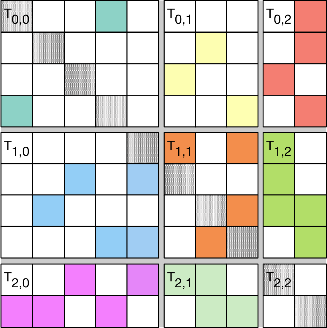
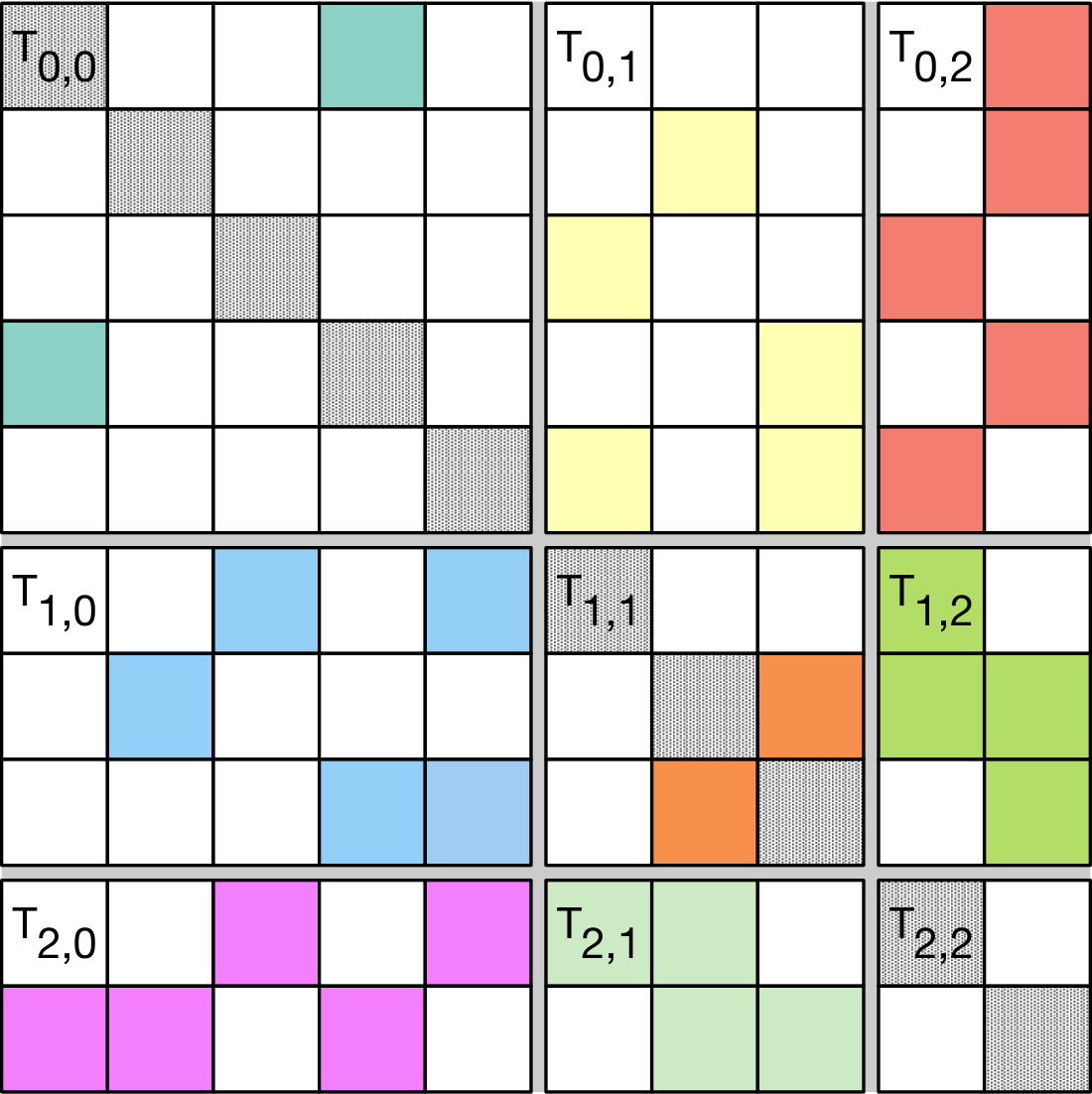
A solution which is perfectly balanced achieves a load imbalance, , of . Figure 1(a) presents a toy example for rectilinear partitioning where , and .
Definition 2.2
Symmetric Rectilinear Partitioning. Given and , symmetric rectilinear partitioning can be defined as partitioning into intervals such that partitions into non-overlapping contiguous tiles where diagonal tiles are squares.
In symmetric rectilinear partitioning, same partition vector, , is used for row and column partitioning. Figure 1(b) presents a toy example for the symmetric rectilinear partitioning where and
In the context of this work, we consider two symmetric rectilinear partitioning problems. The first problem (minLoadImbal, or mLI in short), consists in finding the optimal partition vector, , that minimizes the load imbalance, for a given the matrix and an integer :
The second problem (minNumCuts, or mNC in short), is the dual of the first problem. For a given a matrix, , and an integer, , this problem consists of finding the minimum number of intervals, , that will partition the matrix , where the number of nonzeros in all tiles is bounded by .
3 Related Work
Two-dimensional matrix distributions have been widely used in dense linear algebra. Most of these distributions are cartesian [6]; where the same partitioning vector is used for row and column partition. For sparse and irregular problems finding a good vector that can be aligned with both dimensions is even harder. Therefore, many non-cartesian two-dimensional matrix partitioning methods have been proposed [9, 10, 13] for sparse and irregular problems.
One way to overcome the hardness of proposing one partition vector for rows and columns is to propose a partition vector for rows and columns. This problem is named as rectilinear partitioning [10] (or generalized block distribution [9]). Independently, Nicol [10] and Manne and Sørevik [9] proposed an algorithm to solve this problem that is based on iteratively improving a given solution by alternating between row and column partitioning. These algorithms transform two dimensional (2D) rectilinear partitioning problem into one-dimensional (1D) partitioning problem using a heuristic and iteratively improves the solution. The one-dimensional partitioning problem is built by setting the load of an interval of the problem as the maximum of the load of the interval inside each stripe of the fixed dimension. This refinement technique is presented in Algorithm 1. Here, optimal1DPartition() is a function that returns the optimal 1D partition (which is also known as chains-on-chains partitioning) [12]. Hence, Algorithm 1 returns the optimal 1D row partition for the given column partition .
Computing the optimal solution was shown to be NP-hard by Grigni and Manne [5]. In fact, their proof shows that the problem is NP-hard to approximate within any factor less than . Khanna et al. [7] have shown the problem to be constant-factor approximate.
Rectilinear partitioning may still cause high load-imbalance due to generalization. Jagged partitions (or Semi Generalized Block Distribution [5]) tries to overcome this problem by distinguishing between the main dimension and the auxiliary dimension. The main dimension is split into intervals and each of these intervals partition into rectangles in the auxiliary dimension. Each rectangle of the solution must have its main dimension matching one of these intervals. The auxiliary dimension of each rectangle is arbitrary. Saule et al. [13] present multiple variants and generalization of jagged partitioning.
4 Symmetric Rectilinear Partitioning
We propose five different algorithms for two variants of the symmetric rectilinear partitioning problem. These algorithms can be classified as refinement based and probe-based. In this section, we explain how these algorithms are designed.
4.1 Heuristics for the minLoadImbal problem.
We propose three algorithms for mLI problem. Two of these algorithms, Pick best direction (first) (PBD) and Pick best (in each) iteration (PBI), leverages previously defined refinement technique (see Section 3) into the symmetric rectilinear partitioning problem. Note that these two algorithms have no convergence guarantee. The third algorithm, Probe target cut (PTC), implements another heuristic and probes the minimum load imbalance by moving in partition point in the diagonal of the matrix.
4.1.1 Pick best direction (first) (PBD)
algorithm first applies row-based and column-based refinement independently to simply find the optimal 1D row and column partitions and chooses the one that gives the best load imbalance. Then, iteratively applies the refinement algorithm only in this direction until it reaches the iteration limit () or partition vector does not change significantly (computed using 2-norm). This procedure is presented in Algorithm 2.
The primary advantage of this algorithm is its simplicity. This algorithm can be easily parallelizable like [9, 10]. However, choosing a direction at the beginning may cause missing information that can be gathered from the other direction and the solution may converge to a local optimum quickly.
4.1.2 Pick best (in each) iteration (PBI)
algorithm applies refinement on both row-based and column partitions and always chooses the best partition vector for the next iteration. If that partition vector improves the current best solution, PBI algorithm updates the partition vector that stores the best solution achieved. This procedure is presented in Algorithm 3.
Tracking the load imbalance creates an opportunity to output a better partitioning. However, tracking comes up with a computational cost (). Hence, PBI algorithm is more expensive than PBD algorithm.
4.1.3 Probe target cut (PTC)
probes for the largest possible cut point in each step using a two-dimensional probe algorithm. In refinement based algorithms (PBI and PBD) mapping the problem from two-dimensional space to one-dimension ends up with losing information. PTC algorithm tries to overcome this problem by seeking better cut points in two-dimensional space. In high-level view PTC algorithm is inspired from Nicol’s [10] probe-based one-dimensional partitioning algorithm however PTC algorithm operates on two-dimensional space on diagonal direction in a greedy manner and due to non-convex structure of the problem it doesn’t guarantee an optimal solution. Algorithm 4 presents the two-dimensional probe algorithm. The elements of are found through binary search, , on the matrix. In this algorithm, , searches in the range to compute the largest cut point, such that and for , . Algorithm 4 returns true if at the end partition vector has intervals and the load imbalance is less than . In each step, , PTC algorithm seeks for the largest cut point in the range for which Probe Algorithm 4 returns true. PTC stores the load imbalances of these steps in an array, . After steps, PTC algorithm computes the minimum of and constructs partition vector using a binary search-based approach similar to Algorithm 4. This procedure is presented in Algorithm 5.
Note that, probe algorithm can return false even if there exists a valid partitioning for a given target load imbalance . Because PTC algorithm always searches for the largest cut point and that may cause missing the optimal solution. Hence, this algorithm can also be stuck in a local optimum. However, PTC algorithm considers more cases in a two-dimensional fashion. Therefore, PTC is expected to produce a better partitioning than PBD and PBI algorithms. The major disadvantage of this algorithm is its computational complexity.
4.2 Algorithms for the minNumCuts problem
Given a matrix, , and an integer, , mNC problem aims to output a partition vector, , with the minimum number of intervals, , where the maximum load of a tile in the corresponding partitioning is less then , i.e., . We propose two algorithms to solve this problem. These algorithms are variations of the ones that we propose for mLI problem.
4.2.1 Bound target load (BTL)
algorithm, displayed in Algorithm 6, searches for the minimal intervals using a binary search-based approach (Algorithm 7). In the worst-case, the maximum loaded tile may be filled with nonzeros. Therefore, the initial upper bound for the search space can be defined as . BTL algorithm first reduces this upper bound by using cheap uniform partitioning. Then using this reduced search space, BTL algorithm searches for the minimal intervals using PBD (or PBI) algorithm in the same fashion.
4.2.2 Probe target load (PTL)
algorithm slightly modifies two-dimensional probe algorithm. In each step, , PTL algorithm searches for the largest cut point, in the range that assures all of the tiles until that cut point have less than number of nonzeros, . This procedure is described in Algorithm 8.
4.3 Complexity Analysis.
Table 2 displays the computational complexity of the algorithms we have used in this work. Each iteration of the iterative refinement algorithm [9, 10] (Algorithm 1) has a worst-case complexity of [13] for unsymmetric rectilinear partitioning. The Algorithm is guaranteed to converge with at most iterations. However, as noted in these earlier work, in our experiments we observed that algorithm converges very quickly, and hence for the sake of fairness we have decided to use the same limit on the number of iterations, . For the symmetric case, where , refinement algorithm runs in . and this what we displayed in Table 2.
PBD algorithm first runs Algorithm 1 and then computes the load imbalance. These operations can be computed in and in respectively. In the worst-case, Algorithm 1 is called times. Hence, PBD algorithm runs in .
PBI algorithm runs Algorithm 1 and then computes the load imbalance in each of the iterations. Hence, PBI algorithm runs in .
Probe algorithm (Algorithm 4) does computations in the worst-case to find a cut point. Since there are cut points probe algorithm runs in . PTC algorithm (Algorithm 5) calls Probe algorithm at most times for each . Hence, PTC algorithm runs in .
BTL algorithm initially tries to reduce search space using cheap uniform partitioning, however in the worst-case uniform partitioning may not be able to reduce search space. Hence, in the worst-case BTL algorithm runs times uniform and PBD (or PBI) algorithm. In the worst-case (i.e., when there is fully dense tile). So, BTL algorithm runs in when PBD is used as the secondary algorithm and in when PBI is used as the secondary algorithm.
PTL algorithm has the same complexity with Algorithm 4 and in the worst-case . Hence, PTL algorithm runs in; .
In addition to our proposed algorithms, we use two reference partitioning algorithms as baselines. First, NIC refers to Nicol’s rectilinear partitioning algorithm [10]. This algorithm outputs a partition vector for each dimension, hence it does not output symmetric partitioning. The complexity of this algorithm is provided in [10] and listed in Table 2. Second, UNI refers to uniform partitioning. This is the simplest checker board partitioning, where each tile has an equal number of rows and columns. UNI algorithm runs in constant time.
| Algorithm | Worst-case complexity |
|---|---|
| NIC | |
| PBD | |
| PBI | |
| PTC | |
| BTL+PBD | |
| BTL+PBI | |
| PTL |
| Data Set | Natural Order | Degree Order | RCM Order | ||||||||||||||
| NIC | UNI | PBD | PBI | PTC | NIC | UNI | PBD | PBI | PTC | NIC | UNI | PBD | PBI | PTC | |||
| cit-HepTh | 27,770 | 352,285 | 1.7 | 1.1 | 1.4 | 1.7 | 0.6 | 1.2 | 8.5 | 0.8 | 1.2 | 0.5 | 1.7 | 3.8 | 1.5 | 1.7 | 0.6 |
| email-EuAll | 265,214 | 364,481 | 2.2 | 1.1 | 1.9 | 2.2 | 0.2 | 3.5 | 13.0 | 3.5 | 3.5 | 3.3 | 3.3 | 9.1 | 3.3 | 3.3 | 2.4 |
| soc-Epinions1 | 75,879 | 405,740 | 1.7 | 2.1 | 1.3 | 1.7 | 0.7 | 1.2 | 23.0 | 0.7 | 1.2 | 0.4 | 2.0 | 16.6 | 1.7 | 2.0 | 0.7 |
| cit-HepPh | 34,546 | 420,877 | 1.7 | 0.8 | 1.3 | 1.7 | 0.6 | 1.3 | 6.4 | 0.7 | 1.3 | 0.3 | 1.8 | 3.6 | 1.7 | 1.8 | 0.7 |
| soc-Slashdot0811 | 77,360 | 469,180 | 1.8 | 2.4 | 1.3 | 1.8 | 0.7 | 1.7 | 18.6 | 0.8 | 1.6 | 0.6 | 1.9 | 12.6 | 1.5 | 1.9 | 0.6 |
| soc-Slashdot0902 | 82,168 | 504,230 | 1.8 | 2.6 | 1.3 | 1.8 | 0.7 | 1.6 | 18.5 | 0.7 | 1.6 | 0.4 | 1.8 | 12.4 | 1.4 | 1.8 | 0.3 |
| flickrEdges | 105,938 | 2,316,948 | 1.6 | 1.2 | 1.1 | 1.6 | 0.6 | 1.9 | 25.2 | 1.8 | 1.9 | 1.0 | 2.1 | 21.2 | 2.3 | 2.3 | 1.8 |
| amazon0312 | 400,727 | 2,349,869 | 1.8 | 1.1 | 1.6 | 1.8 | 0.4 | 1.8 | 2.5 | 1.2 | 1.8 | 0.7 | 2.0 | 2.0 | 1.9 | 2.0 | 0.8 |
| amazon0505 | 410,236 | 2,439,437 | 1.8 | 1.2 | 1.6 | 1.8 | 0.4 | 1.8 | 2.5 | 1.2 | 1.8 | 0.6 | 2.0 | 1.9 | 1.9 | 2.0 | 0.7 |
| amazon0601 | 403,394 | 2,443,408 | 2.1 | 3.0 | 1.9 | 2.1 | 0.6 | 1.9 | 2.4 | 1.2 | 1.9 | 0.6 | 2.0 | 2.0 | 1.9 | 2.0 | 0.8 |
| scale18 | 174,147 | 3,800,348 | 1.7 | 1.4 | 0.9 | 1.7 | 0.8 | 1.8 | 22.2 | 1.1 | 1.8 | 1.1 | 1.9 | 17.2 | 1.0 | 1.9 | 0.7 |
| scale19 | 335,318 | 7,729,675 | 2.2 | 6.7 | 2.2 | 2.2 | 1.1 | 2.4 | 13.5 | 2.0 | 2.4 | 1.0 | 2.2 | 9.9 | 2.0 | 2.2 | 0.6 |
| as-Skitter | 1,696,415 | 11,095,298 | 1.7 | 1.6 | 1.0 | 1.7 | 0.9 | 1.8 | 23.7 | 1.0 | 1.8 | 1.0 | 1.9 | 18.5 | 1.3 | 1.9 | 1.2 |
| scale20 | 645,820 | 15,680,861 | 1.7 | 1.4 | 1.0 | 1.7 | 0.9 | 1.8 | 24.1 | 1.0 | 1.8 | 1.0 | 1.9 | 19.4 | 1.3 | 1.9 | 1.2 |
| cit-Patents | 3,774,768 | 16,518,947 | 1.9 | 2.2 | 1.8 | 1.9 | 1.0 | 1.6 | 6.7 | 1.2 | 1.6 | 0.7 | 2.0 | 3.3 | 1.9 | 2.0 | 0.7 |
| scale21 | 1,243,072 | 31,731,650 | 1.7 | 1.3 | 1.0 | 1.7 | 0.9 | 1.8 | 24.8 | 1.0 | 1.8 | 1.0 | 1.9 | 20.4 | 1.0 | 1.9 | 0.8 |
| soc-LiveJournal1 | 4,847,571 | 42,851,237 | 1.9 | 7.7 | 1.7 | 1.9 | 0.4 | 1.3 | 15.6 | 1.0 | 1.3 | 0.6 | 1.8 | 7.2 | 1.6 | 1.8 | 0.5 |
| wb-edu | 9,845,725 | 46,236,105 | 3.4 | 4.0 | 3.4 | 3.4 | 3.2 | 2.6 | 13.2 | 2.6 | 2.6 | 0.5 | 3.0 | 4.0 | 3.0 | 3.0 | 1.7 |
| 61,578,414 | 1,202,513,046 | 1.7 | 2.0 | 1.2 | 1.7 | 0.3 | 2.3 | 23.1 | 2.1 | 2.3 | 1.7 | 1.5 | 5.2 | 1.4 | 1.5 | 1.0 | |
| friendster | 65,608,366 | 1,806,067,135 | 1.3 | 2.7 | 1.1 | 1.3 | 0.6 | 1.2 | 17.5 | 0.6 | 1.2 | 0.4 | 1.3 | 10.6 | 1.0 | 1.3 | 0.5 |
| Geomean: | 1.8 | 1.9 | 1.4 | 1.8 | 0.7 | 1.8 | 12.2 | 1.2 | 1.8 | 0.7 | 2.0 | 7.5 | 1.6 | 2.0 | 0.8 | ||
5 Experimental Evaluation
The partitioning algorithms presented for mLI and mNC problems are implemented in the C++ programming language and compiled with GCC version 7.2. The experiments are conducted on a server that has four, 14-core Intel Xeon E7-4850 2.20GHz processors, 2TB of memory, 1TB disk space, running Ubuntu GNU/Linux with kernel 4.8.0.
We have performed an extensive evaluation of the proposed algorithms on 16 different real-world and 4 different synthetic (RMAT) graphs coming from SuiteSparse Matrix Collection (formerly known as UFL) [1], SNAP 11 1 SNAP Datasets: http://snap.stanford.edu/data, and DARPA Graph Challange 22 2 GraphChallenge Datasets: https://graphchallenge.mit.edu/data-sets. Properties of these datasets, along with the load balances found by different algorithms on different layouts of these matrices are presented in Table 3. In the experiments, we used and .
In our experiments, we included three different vertex ordering techniques before giving the adjacency matrix to respective partitioner: the natural order of the vertices (NAT), degree-based ordering of the vertices (DEG) and Reverse Cuthill McKee (RCM) based ordering of the vertices. Figure 2 illustrates these orderings along with the adjacency matrix representations for a toy graph.
5.1 Load imbalance evaluation.
We first evaluate the proposed algorithms for the mLI problem. Table 3 reports load imbalances of five different algorithms; NIC, UNI, PBD, PBI, and PTC, on three different vertex ordering techniques, NAT, DEG and RCM for each graph. In this experiment we chose . Hence, every graph is partitioned into tiles. In Table 3, the best load imbalance for a graph instance is highlighted using the green color. As expected, PTC algorithm gives the best load imbalance in every graph instance. The best load imbalance among with the other four algorithms; NIC, UNI, PBD, and PBI, for each vertex ordering are highlighted using yellow color. PBD algorithm gives the best performance among these four algorithms in of the graph instances. PBI and NIC algorithms give very similar load imbalances.
In Table 3, the last row presents geometric means of the five different algorithms on three different vertex orderings. As shown in the table, the geometric means of PTC algorithm on NAT, DEG and RCM vertex orderings are , and , respectively. These results show that PTC algorithm is more resistant to the vertex order, and hence, it can produce partitioning with similar qualities. On the other hand, we observe a significant change in load imbalance (up to ) for refinement based algorithms depending on the vertex order. As expected, uniform partitioning performs poor on DEG vertex order due to higher density in the bottom right portion of the adjacency matrix.
5.2 Algorithm evaluation.
We evaluate relative load imbalance performances of NIC, UNI, PBD, PBI and PTC algorithms. The aim is to illustrate the efficiency of the proposed algorithms with respect to NIC and UNI. In this experiment, NAT vertex ordering is used and we choose . Figure 3 illustrates the performance profiles of the algorithms for different values. In the performance profiles, we plot the number of the test instances (y-axis) in which an algorithm obtains a load imbalance on an instance that is no larger than times (x-axis) the best load imbalance found by any algorithm for that instance [2]. Therefore, the higher a profile at a given value, the better an algorithm is. We observe that in all cases (Figure 3(a)-Figure 3(c)) PTC algorithm gives the best performance in the majority of the test instances. PBD algorithm becomes the second-best algorithm. We also observe that NIC and PBI algorithms have almost identical profiles. Both of these algorithms consider row-based and column-based directions in each iteration. Therefore, probably they fall into the same local optimum and stuck. As expected UNI algorithm performs the worst because of the irregularity of the graphs.
5.3 Visualization of block distributions.


In Figure 4, we present density maps of NIC, UNI, PBD and PTC based partitioning where on soc-LiveJournal1 and friendster graphs. The same color range used in all plots and darkness of the color of a tile is proportional to the number of nonzeros inside the tile. In this experiment, NAT vertex ordering is used. Percentages presented for each tile present percentage of the number of nonzeros within a tile. Note that in these figures tiles are mapped into a grid for a better visualization. hence NIC algorithm outputs a rectilinear partitioning, therefore, there can be nonzero tiles under diagonal tiles. Figure 4(d) visually supports our previous findings; PTC algorithm produces better partitioning (closely colored tiles) and UNI gives the worst (too much variance between tile colors) and PBD performs slightly better then NIC algorithm.
5.4 Number of cut evaluation.
In this experiment, we evaluate performances of BTL and PTL algorithms, proposed for the mNC problem. Table 4 reports the number of cuts found by these algorithms for different graphs. We choose for each graph. UNI algorithm outputs the minimum number of cuts that can be gathered using uniform partitioning. In Table 4 for each graph, the minimum number of cuts is highlighted using a green color. We observe that NAT vertex ordering has a lower number of cuts in general due to the more uniform distribution of the nonzeros. On the other hand algorithms output higher number of cuts using RCM vertex ordering, because RCM creates denser regions while trying to make nonzeros appear near diagonal. As expected UNI partitioning performs the worst.
| Data Set | NAT | DEG | RCM | ||||||
|---|---|---|---|---|---|---|---|---|---|
| UNI | BTL | PTL | UNI | BTL | PTL | UNI | BTL | PTL | |
| cit-HepTh | 5 | 5 | 4 | 7 | 6 | 5 | 6 | 6 | 5 |
| email-EuAll | 5 | 5 | 4 | 7 | 6 | 5 | 6 | 6 | 5 |
| soc-Epinions1 | 8 | 6 | 4 | 7 | 6 | 5 | 6 | 6 | 5 |
| cit-HepPh | 15 | 6 | 5 | 35 | 7 | 6 | 20 | 6 | 5 |
| soc-Slashdot0811 | 5 | 5 | 4 | 13 | 6 | 5 | 9 | 6 | 5 |
| soc-Slashdot0902 | 5 | 5 | 4 | 16 | 5 | 5 | 9 | 6 | 4 |
| flickrEdges | 7 | 6 | 5 | 15 | 5 | 5 | 8 | 6 | 5 |
| amazon0312 | 5 | 5 | 5 | 120 | 8 | 8 | 25 | 8 | 7 |
| amazon0505 | 5 | 5 | 5 | 71 | 6 | 5 | 48 | 6 | 6 |
| amazon0601 | 7 | 5 | 5 | 46 | 5 | 5 | 21 | 5 | 5 |
| scale18 | 6 | 5 | 5 | 82 | 6 | 6 | 36 | 6 | 6 |
| scale19 | 6 | 5 | 5 | 99 | 6 | 5 | 44 | 6 | 6 |
| as-Skitter | 6 | 5 | 5 | 127 | 5 | 5 | 52 | 6 | 6 |
| scale20 | 6 | 5 | 5 | 166 | 5 | 5 | 57 | 6 | 6 |
| cit-Patents | 6 | 5 | 5 | 86 | 5 | 4 | 34 | 6 | 5 |
| scale21 | 14 | 6 | 4 | 63 | 5 | 5 | 15 | 6 | 5 |
| soc-LiveJournal1 | 7 | 6 | 5 | 50 | 5 | 5 | 23 | 6 | 5 |
| wb-edu | 7 | 6 | 5 | 50 | 5 | 5 | 21 | 6 | 5 |
| 6 | 5 | 5 | 275 | 7 | 6 | 14 | 5 | 5 | |
| friendster | 10 | 8 | 8 | 33 | 7 | 5 | 9 | 8 | 6 |
5.5 Execution time evaluation.
Table 5 shows the execution time behavior of six algorithms; NIC, PBI, PBD, PTC, BTL, and PTL, on the largest five graphs in our dataset listed in Table 3. We observe that, for mNC problem both BTL and PTL algorithms’ execution times are similar. For mLI problem, for the smaller three graphs, both PBI and PBD algorithms’ execution time is about 1.5 times slower than NIC. On largest two graphs PBD is the fastest algorithm. Given the computational complexities of the algorithms in Table 2, as expected PTC algorithm was the slowest of all, due to too many prefix sum lookups on the matrix. Please note that, Table 2 assumes linear lookup for a given partition vector and require linear space. We first developed a naive implementation with such linear lookup, which was two to three orders of magnitude slower than than other algorithms. To decrease the lookup complexity for PTC algorithm we used a sparse prefix sum data structure inspired from the Fenwick tree [3], that can query the matrix in logarithmic time but requires times more space. With that data structure PTC algorithm now to times slower than NIC algorithm.
| Data Set | mLI | mNC | ||||
| NIC | PBI | PBD | PTC | BTL | PTL | |
| scale21 | 0.9 | 1.4 | 1.6 | 17.9 | 5.3 | 3.9 |
| soc-LiveJournal1 | 1.7 | 2.4 | 4.5 | 26.7 | 245 | 269 |
| wb-edu | 1.8 | 2.6 | 2.4 | 7.19 | 14.7 | 17.1 |
| 81 | 126 | 42 | 2,817 | 190 | 186 | |
| friendster | 145 | 235 | 70 | 6,700 | 245 | 269 |
6 Conclusion
In this work, we proposed different heuristics for symmetric rectilinear partitioning problem and present a thorough experimental evaluation showing the effectiveness of the proposed algorithms. Even though our problem definition is more restricted, in our experiments, we observed that our proposed algorithms give better load-imbalance than Nicol’s [10] state-of-the-art rectilinear partitioning algorithm in every test instances. PTC algorithm gives the best load imbalance in the majority of the test instances and PBD algorithm is the second-best algorithm. PBI algorithm’s performance is almost identical to NIC.
As future work, we are working on decreasing the space requirements of our sparse prefix sum data structure and also decreasing the number of lookups that PTC performs. In addition, we will also investigate approximation techniques, and parallelization of the algorithm.
7 Acknowledge
We would like to extend our gratitude to M. Fatih Balin for his valuable comments and sharing his sparse prefix sum data structure code with us.
References
- [1] T. A. Davis and Y. Hu, The University of Florida sparse matrix collection, ACM Transactions on Mathematical Software (TOMS), (2011), p. 1.
- [2] E. D. Dolan and J. J. Moré, Benchmarking optimization software with performance profiles, Mathematical programming, 91 (2002), pp. 201–213.
- [3] P. M. Fenwick, A new data structure for cumulative frequency tables, Software: Practice and Experience, 24 (1994), pp. 327–336.
- [4] G. Gill, R. Dathathri, L. Hoang, and K. Pingali, A study of partitioning policies for graph analytics on large-scale distributed platforms, Proceedings of the VLDB Endowment, 12 (2018), pp. 321–334.
- [5] M. Grigni and F. Manne, On the complexity of the generalized block distribution, in International Workshop on Parallel Algorithms for Irregularly Structured Problems, 1996, pp. 319–326.
- [6] B. Hendrickson, R. Leland, and S. Plimpton, An efficient parallel algorithm for matrix-vector multiplication, International Journal of High Speed Computing, 7 (1995), pp. 73–88.
- [7] S. Khanna, S. Muthukrishnan, and S. Skiena, Efficient array partitioning, in International Colloquium on Automata, Languages, and Programming, 1997, pp. 616–626.
- [8] J. G. Lewis, D. G. Payne, and R. A. van de Geijn, Matrix-vector multiplication and conjugate gradient algorithms on distributed memory computers, in Proceedings of IEEE Scalable High Performance Computing Conference, IEEE, 1994, pp. 542–550.
- [9] F. Manne and T. Sørevik, Partitioning an array onto a mesh of processors, in International Workshop on Applied Parallel Computing, 1996, pp. 467–477.
- [10] D. M. Nicol, Rectilinear partitioning of irregular data parallel computations, Journal of Parallel and Distributed Computing, 23 (1994), pp. 119–134.
- [11] D. P. O’leary and G. Stewart, Data-flow algorithms for parallel matrix computation, Communications of the ACM, 28 (1985), pp. 840–853.
- [12] A. Pınar and C. Aykanat, Fast optimal load balancing algorithms for 1D partitioning, Journal of Parallel and Distributed Computing, 64 (2004), pp. 974–996.
- [13] E. Saule, E. O. Bas, and Ü. V. Çatalyürek, Load-balancing spatially located computations using rectangular partitions, Journal of Parallel and Distributed Computing, 72 (2012), pp. 1201–1214.
- [14] A. Yaşar, S. Rajamanickam, J. W. Berry, M. M. Wolf, J. Young, and Ü. V. Çatalyürek, Linear algebra-based triangle counting via fine-grained tasking on heterogeneous environments, in IEEE High Performance Extreme Computing Conference (HPEC), 2019.