Appearances of the Birthday Paradox in High Performance Computing
Abstract
We give an elementary statistical analysis of two High Performance Computing issues, processor cache mapping and network port mapping. In both cases we find that, as in the birthday paradox, random assignment leads to more frequent coincidences than one expects a priori. Since these correspond to contention for limited resources, this phenomenon has important consequences for performance.
1 Introduction
The birthday paradox is not so much a paradox as an unexpected result. It expresses that collisions between unlikely events can be more likely than expected a prima facie. In the phenomenon that gives it its name, we consider the probability that in a set of people a pair will have the same birthday. The paradoxical aspect is that, for a given probability, the value of is rather lower than one would expect: for a chance it is enough to have , and gives a chance.
In this paper we give two examples of such collisions from the field of HPC (HPC), which is normally not associated with statistical reasoning. We phrase the problem as follows: we consider random assignments of entities to open slots; in cases where according to the ‘pigeonhole principle’ a conflict-free assignment is possible, in practice we will still get conflicts. We then consider two common examples from the field of HPC, in particular cache associativity and network switch oversubscription. In both these phenomena we show that performance aspects can be given a simple statistical analysis. We claim no particular novelty for this analysis, but we hope that our exposition may provide both inspiring examples to statisticians and an illustration of the use of statistics to HPC practitioners.
2 Appearance #1: Memory caches
2.1 Background
Since the late 1980’s, the operating frequency of computer processors has been increasing at a significantly faster rate than the operating frequency of the computer’s main memory. To reduce processor stalls while waiting on memory accesses, ‘caches’ have been added to almost all processors. Caches are small amounts of high-speed memory that transparently retain the data from recently accessed memory locations. (They also retain the knowledge of where the data originated.) Accessing a memory location that is mirrored in the cache allows full-speed operation, while accessing a memory location that does not have valid data in the cache typically results in lower performance, since the processor stalls waiting for data to arrive.
Since these high-speed caches are relatively small, the data from the newly accessed memory location also displaces data from some previously accessed memory location in the cache. This potentially lowers performance again, since the displaced data may be needed in the near future. Achieving high performance thus requires algorithms that have high rates of data re-use on subsets of the data that ‘fit’ into the cache.
2.2 Address mapping
Our analysis of this data re-use, and hence code performance, will focus on the mapping function that translates memory addresses into cache locations. (Our discussion is a simplification, in that we ignore the further memory access history of the application, and other non-trivial details of the cache implementation.)
The mapping function is used every time the processor performs a memory access: the memory address is translated in order to determine which cache index to query. The cache control logic compares the memory address requested by the processor with the memory address held in that cache location. If the addresses match, the data from the cache is returned to the processor. If the addresses do not match, the request must be sent to the main memory to retrieve the correct data. When the data is returned from memory, the cache replaces the previous data held at this index with the new data and updates the memory address at this index with the address of the newly loaded data.
2.3 Direct mapping
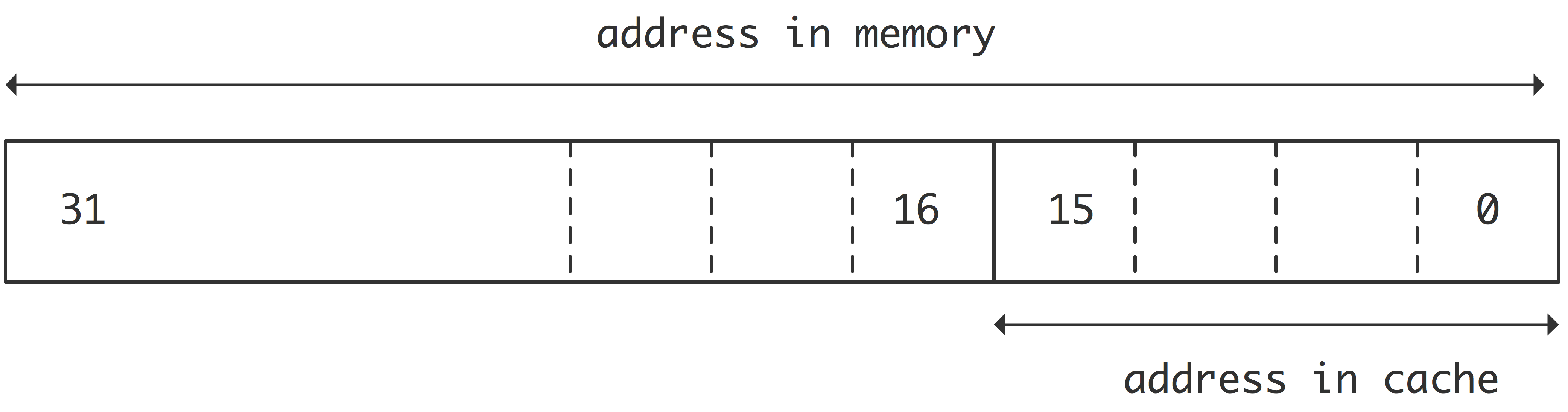
From a hardware implementation perspective, the easiest way to map memory locations to cache locations is with a power-of-2 modulo function. For a cache with locations, the cache ‘index’ consists of the first (low-order) bits of the memory address. (Figure 1 illustrates taking the last 16 bits of a 32 bit address.) At each location, the cache stores a block of data, the corresponding memory address, and a small amount of additional data to track validity and other attributes.
It is clear from this description that such a cache can hold data blocks for re-use – but only if the set of memory addresses being accessed contains no duplicate cache index mappings. In some cases, this can actually be guaranteed with information available to the user. For the direct-mapped cache described above, any set of contiguous memory locations will map to each cache index exactly once, guaranteeing freedom from conflicts – though it should be noted that user-visible addresses are subject to a minimum of one level of address translation, which limits the size of contiguous regions in machine-dependent ways.

On the other hand, addresses at a distance of from each other have the same lower address bits, and will then be mapped to the same cache location. (This is illustrated in figure 2, which models the simultaneous traversel of two matrix rows.) Such a code will run much slower.
However, in many cases cache mappings are not visible to users in any useful way, either because of virtual-to-physical address translations (controlled by the operating system and not by the user), or because the cache indexing function is complex and undocumented, or because the set of addresses being accessed is dynamically randomized (e.g., with dynamically repartitioned graph structures). In these cases, the mapping of user-visible memory addresses to cache indices takes on a random component, and statistical analysis becomes essential.
This brings us to the ‘birthday problem’. Given a direct-mapped cache of size and a set of user-visible memory addresses (that map to set of pseudo-random cache indices), what can be derived about the probability of conflict of various degrees?
As the number of sets grows, the probability “zero conflicts” approaches zero, but it also becomes less relevant. A more relevant metric might be the probability of getting a set of random addresses with no more than some fixed percentage of conflicts – maybe N/8 to approach 90% hit rates (but see the caveat above about how many cache misses occur due to each conflict). For a set of addresses that are accessed only once per repetition and for which the order is the same in each repetition, the number of hits is the number of sets with exactly one cache line mapping — all sets with 2 or more mappings miss every time.
Problem statement If we have a cache of locations, and we have a working set of memory words, some of these words will be mapped to the same cache location, so we have an effective cache size that is smaller than elements. We will investigate what the expected effective cache size is.
2.4 Associative caches

The common solution taken to mitigate mapping conflicts is to make caches multi-way associative: addresses are no longer uniquely mapped, but rather to a ‘set’ of locations in the cache. We call a cache -way associative if each set has elements. This means that a -way collision can be resolved since identically mapped address fill the locations of a set. This is illustrated in figure 3. For instance, with , our code can traverse one output and three input arrays that are at an otherwise conflicting offset from each other.
2.5 Model formulation
We have just motivated the design of associative caches from traversing multiple arrays in one algorithm. However, not all memory access is this systematic. Thanks to out-of-order execution, multi-threading, virtual-to-physical address translation, and any intrinsically unstructured nature of the application, we can also consider loads from memory as a random stream of address requests. The question to analyze becomes then, what is the hit/miss ratio of a random stream of addresses as a function of , the associativity of the cache.
Increasing the value of is desirable since it decreases the likelihood of conflicts. However, it also increases the cost, both in design, construction, and energy usage of the electronics, as well as possibly depressing the allowable clock speed. Our statistical analysis is therefore part of the cost/benefit analysis of processor design.
We model our cache as follows: we assume a cache with locations, and -way associativity, giving sets. An address in main memory, is mapped to the set , and each set can store items. The question is then, given random addresses, what is the likelihood that more than addresses map to the same . This is a generalization of the ‘birthday paradox’, which in this context corresponds to and .
2.6 Analysis
As with the regular birthday paradox, to analyze how likely collisions are, we examine the complement: the probability of random mappings being collision free. First we look at the expected number of addresses stored if addresses are mapped where is the number of sets, and we have -way associativity.
Since the addresses are random, and all sets equally likely, we use the linearity of the expectation value to get our basic equation for the expectation value of the number of items stored in a cache with sets and locations :
Our basic random variables are
where we note that .
We derive by splitting it into two cases. We observe that has a maximum value of , the associativity, but can be larger. If set contains fewer than elements, it means that exactly that many addresses were mapped to it, and . On the other hand, if set contains elements it means that or more addresses were mapped to it, and the case corresponds to the set of cases .
This gives:
| (1) | ||||
| (2) | ||||
| \unitindenttake complement: | ||||
| (3) | ||||
| \unitindentenumerate cases | ||||
| (4) | ||||
| (5) | ||||
| \unitindentassuming is binomial, with trials and chance of success | ||||
| (6) | ||||
| \unitindentsimplify, using : | ||||
| (7) | ||||
Example: for a cache of 1000 elements the number of elements stored for a variety of associativities is:
| associativity | 1 | 2 | 3 | 4 | 10 | 50 | 100 |
| expected working set size | 632 | 729 | 775 | 805 | 875 | 945 | 962 |
Remark. Since we essentially compute the expected number of stored elements in a set, using a larger cache, while keeping associativity, constant, only increases the number of sets. Therefore the expected working set size is a fraction of the cache size that depends on the associativity, not on the number of sets. Under further assumptions on code behavior, such as a decaying ‘rate of rereference [4]’ we get a miss rate that decays with cache size.
2.7 Working set sizes
.
Now, if we want to prevent cache conflicts in other than a very regular application we need to use a working set that is smaller than the cache size. The above formula for expected value is a good guideline, but what is the penalty for getting conflicts regardless? For a single computer a slight loss of efficiency is no emergency, for many processes running a fairly tightly coupled application, this performance degradation holds up the overall computation. Thus we could ask, given a set of processors, what size working set can we safely adopt to have a chance of conflicts . This is of course relevant for clusters, which can have many thousands of processors, but we note that current Intel Xeon processors can have up to 28 cores, making this question already relevant on a single-computer scale.
We first analyze the chance of having no conflicts when random addresses are assigned to a cache of slots and -way associativity, where . This is the number of possible conflict-free mappings of addresses, divided by the total number of mappings, which is .
Let be the number of sets with addresses stored in them. While in principle all can range , there are also complicated relations between them, giving recursively defined bounds. We say that can range from to , which we will now compute. If is the number of addresses mapped to slots with addresses mapped to them, we have and . With this we get11 1 The computation for is a special case as can take only one value: and .
Now for a given set of indices we count the number of permutations, giving us finally:
| (9) |
If we apply this analysis, we see that a probably-conflict-free working set will be quite small. For instance, a cache with 4000 elements and 4-way associativity will have an expected working set of around 3200 elements. However, randomly assigning that many addresses will in fact have a probability of only of no conflicts.
This table gives the probability of no-conflicts for various working set sizes, in a 4-way associative cache of 4000 elements.
| working set size | |||||
|---|---|---|---|---|---|
| no-conflict probability |
Looking at this another way, we can ask if a certain fraction of the cache size is a safe working set size. It turns out that for a fixed fraction the probability of no conflicts also goes down quickly with cache size.
| cache size | |||||
|---|---|---|---|---|---|
| no-conflict probability |
Having simultaneously low probability on hundreds or thousands of processors will give an even lower number for the feasible working set size.
In this case we cannot but draw the conclusion that our analysis is overly pessimistic, since it assumes totally randomly generated addresses. In practice, programmers will use optimization techniques such as blocking to make the memory use decidedly more regular.
Computation remark Equation (9) takes some care to compute. While both numerator and denominator are integers, and languages such as python have support for very large integers, the quotient is a real number, and the integers involved are too large to convert to real. Hence all product have to be computed as powers of sums of logarithms.
2.8 Illustration from concrete examples
2.8.1 Modern Intel Xeon processors
In order to discuss a real-life cache we need to point out that computer memory, as well as cache memory, is organized in ‘cachelines’, which are the smallest units of memory that can be moved about. That is, if a program references a certain byte in memory, the cacheline containing that byte is moved into cache. The typical cacheline these days is 64 bytes, or 8 double precision numbers, long.
Now we can consider the L1 (data) cache of modern Intel Xeon processors, which has a size of 32Kib, i.e., bytes. The typical associativity is 8, meaning that 12 bits of an address are used to determine the set. However, assignment is done per cacheline; not per byte. Since 6 of the address bits are used to determine the location of a byte in the cacheline, the actual assignment uses the remaining (most significant) 6 bits, meaning that the cache has 64 sets.
By the above analysis, we expect 441 out of 512 generated cachelines to remain in the cache.
2.8.2 Memory as cache in recent Intel processors
In recent Intel processors, parts of the DDR4 memory can be configured as direct mapped cache. The first architecture to do this was the KNL (KNL) processor, but the same principle applies to the new ‘Intel Optane DC Persistent Memory’.

It was observed that codes using this cache mode had a decreasing performance as as function of time. To understand this, it is necessary to take into account the virtual-to-physical address translation22 2 Running programs refer to a memory address space expressed in virtual addresses; the page table translates to actual physical memory addresses., which is gradually established as programs run. Initially, this translation fills up the cache linearly, so there are no cache conflicts. Then, as the cache is full – which can take a while since this cache is typically 16Gbyte – the direct mapped behavior becomes gradually apparent.
For instance, figure 4 shows how bandwidth (measured by the Stream benchmark [7]), which we use as a proxy for cache hit rate, degrades as a function of uptime of the processor: as time goes on the random mapping of pages turns orderly memory access into random memory access. In the context of supercomputer clusters, such as Stampede 2 at the Texas Advanced Computing Center, this was solved by reordering the list of free pages after each user job.
2.9 Discussion and related work
We have shown that a model based on simple statistical tools can often get close to observed behaviour. However, we had to make a number of simplifying assumptions that make our story sometimes unduly pessimistic. For practical processor design, therefore, one usually relies on sophisticated modeling software, such as CACTI [12].
An early review paper on cache design [11] used both simulations based on program traces, and gave a statistical result on the likelihood of referencing data already in cache. The latter uses the ‘LRU Stack Distance’ model, which is based on the notion that, given a reference to a certain item an memory, other items become more likely to be referenced next. The resulting formula shows similarities to our result ().
The classic computer architecture reference [5] uses simulation results from traces such as the Spec benchmarks. Unlike our simplified model, it includes factors such as the time required for looking up whether a data reference is a cache hit or miss.
The concepts behind caching were already explored a few decades earlier in the context of paging [9]. Paging is usually presented as ‘moving memory blocks – or: pages – to disc when they are not in use, but turning this story upside down, we see that it is essentially the same phenomenon. A program can use addresses out of a potentially large logical address space, and pages get placed on physical addresses in main memory. If a program uses a larger address space than there is physical memory, or if multiple programs run simultaneously, memory pages can be evicted to disc, which serves as bulk memory.
3 Appearance #2: Port mapping in supercomputer clusters
3.1 Background
Supercomputer clusters typically contain hundreds to thousands of ‘nodes’, each containing a smal number of processor chips, typically 1 or 2 or 4. Since the cost of connecting each of nodes to every other node is prohibitive, there is usually a network involved that limits the number of connections to less than , while still offering enough bandwidth for typical HPC workloads. One popular network topology is the ‘grid’ where each node has a fixed, low number of connections that arranges the nodes into the topological equivalent of a grid. A typical grid network is topologically three-dimensional, but the K-computer has a 6-dimensional network.

The other currently popular topology is of a multi-stage network, built up out of individual switching elements. This is known as a Banyan network [2], a ‘butterfly exchange’ network33 3 http://en.wikipedia.org/wiki/BBN_Butterfly, a ‘fat-tree’ [6] or a ‘Clos network’ [1]. Figure 5 depicts a network where each switching element has four ‘ports’, but in practice a typical number is on the order of 30–40. The top level switches have all their ports facing into the network, while the intermediate ones designate half of their ports as ‘input’ and half as ‘output’ ports.
While mathematically the number of levels of such a network is a logarithm of the number of processors, in practice the number of levels is three, or in rare cases four. This is due to the high port count, which functions as the base of the logarithm, and the existence of multiple top level nodes.

As a practical illustration, figure 6 shows three (out of five) central switch cabinets of the Stampede2 cluster44 4 https://www.tacc.utexas.edu/systems/stampede2, recognizable by the blue cabling. These cabinets contain both the top-level ‘spine cards’, as well as the intermediate level ‘leaf cards’. The ‘leaf switches’ connected to the processors are part of the processor cabinets.
3.2 Problem statement

The design of the network is not uniquely determined by the number of processors and the number of ports on a node. At the top level of the network (confusingly, also known as the root nodes) all ports are connected to the next, intermediate, network layer. However, at the intermediate layers there is the possibility to trade ‘outbound’ ports for ‘inbound’ ones, only keeping the total number of ports constant. This process is known as ‘oversubscription’, since it means that there can be more traffic going into the switch than is going out. Oversubscription is an obvious cost saving measure, since it cuts down on the number of switching elements needed at higher levels.

However, oversubscription means that we have to map incoming connections to output ports, and so there is obviously contention if all nodes are sending at the same time. Figure 7 shows a simplified network where we have done away with all intermediate stages and only show sending and receiving processors plus the switches they are directly attached to. In this figure we route traffic for six processors through four outbound ports on a 10-port switch; the arrows show the mapping from target processor to output port.
Now consider that, if nodes are sending through the switch, we have theoretically enough capacity, but the ‘static routing’ used by most clusters means that some choices of destination nodes will give contention for the output ports. Figure 8 shows two sets of destination processors; the green set has no contention, while the red set does. Here we have another case where according to the pigeon-hole principle a unique assignment should be possible, but where in practice conflicts are likely.
This is then our problem: to analyze the chance of collision-free traffic if the number of simultaneous messages equals that of the number of output ports. Having simultaneous messages is an expected scenario in practice, since scientific application often behave in a synchronized manner, even if they do not have explicit synchronization mechanisms.
3.3 Analysis
In the traditional birthday problem, we have a large space of possibilities and a small number of picks from that space. Here we have a much smaller space of possibilities, and the number of picks is equal to it. We could model this as follows: consider birth months rather than days, and we have more than 12 people. Picking 12 out of these, what is the chance that no two share a birth month?
Let be the number of destination nodes, the number of ports, and be the number of requests. Each port has 1 or 2 associated destinations, so ports will have 0, 1 or 2 requests. If a port has 2 requests, that is a collision. Let be the number of collisions. We will categorize ports as either single or double, depending on whether one or two messages target them. There will be double ports and single. If order of destination requests is not considered, there are ways of choosing destinations of the without other restrictions. The number of ways of making requests without having collisions is found by counting the number of ways that each port has exactly one request. With order not considered, there is one destination choice for each single and 2 for each double port, This yields unique port configurations, so the probability of no collisions is .
An interesting way to get insight in this formula is to use
Using that for , we get (for ):
The case is not practical, since the number of ports on a switch is typically even. That leaves the second case as the minimal one, and in terms of :
In a 30-port design, a quite reasonable size, the minimal oversubscription is then 16 input ports and 14 output ports. In a random communication with 14 sources and destinations this gives a chance of no collisions of .
3.4 More discussion
In the above discussion we made it sound as if a message chooses a port. In practice, the port is ‘destination routed’: the port is statically determined by the message destination according to the ‘routing tables’. These map, on each switching element, the possible destinations to the output port on that switch. While it would be possible to configure a program run so as to take advantage of the routine tables, in practice this is infeasible, the more so since conflicts with other users’ programs are upredictable.
This particular instance of the birthday paradox is alleviated with dynamic routing, which will be available on the TACC Frontera machine, to come online medio 2019.
References
- [1] Charles Clos. A study of non-blocking switching networks. Bell System Technical Journal, 32:406–242, 1953.
- [2] T. Y. Feng. A summary of interconnection networks. IEEE Computer, 14:12–27, 1981.
- [3] Trevor Fisher, Derek Funk, and Rachel Sams. The birthday problem and generalizations. Carlton College, Mathematics Comps Gala, May 21st, 2013.
- [4] A. Hartstein, V. Srinivasan, T. R. Puzak, and P. G. Emma. Cache miss behavior: is it ? In Proceedings of the 3rd conference on Computing frontiers, CF ’06, pages 313–320, New York, NY, USA, 2006. ACM.
- [5] John L. Hennessy and David A. Patterson. Computer Architecture, A Quantitative Approach. Morgan Kaufman Publishers, 3rd edition edition, 1990, 3rd edition 2003.
- [6] Charles E. Leiserson. Fat-Trees: Universal networks for hardware-efficient supercomputing. IEEE Trans. Comput, C-34:892–901, 1985.
- [7] John D. McCalpin. Stream: Sustainable memory bandwidth in high performance computers. Technical report, University of Virginia, Charlottesville, Virginia, 1991-2013. A continually updated technical report.
- [8] Michael J. McGlynn and Steven A. Borbash. Birthday protocols for low energy deployment and flexible neighbor discovery in ad hoc wireless networks. In Proceedings of the 2Nd ACM International Symposium on Mobile Ad Hoc Networking &Amp; Computing, MobiHoc ’01, pages 137–145, New York, NY, USA, 2001. ACM.
- [9] A.C. McKellar and E.G. Coffman jr. Organizing matrices and matrix operations for paged memory systems. J. ACM, 12:153–165, 1969.
- [10] E. H. Mckinney. Generalized birthday problem. The American Mathematical Monthly, 73(4):385–387, 1966.
- [11] Alan Jay Smith. Cache memories. ACM Comput. Surv., 14(3):473–530, September 1982.
- [12] D. Tarjan, S. Thoziyoor, and N. P. Jouppi. CACTI 4.0. Technical Report HPL-2006-86, HP Labs, 2006.