The condition number of
Riemannian approximation problemsThanks: Submitted to the editors.
Abstract
We consider the local sensitivity of least-squares formulations of inverse problems. The sets of inputs and outputs of these problems are assumed to have the structures of Riemannian manifolds. The problems we consider include the approximation problem of finding the nearest point on a Riemannian embedded submanifold from a given point in the ambient space. We characterize the first-order sensitivity, i.e., condition number, of local minimizers and critical points to arbitrary perturbations of the input of the least-squares problem. This condition number involves the Weingarten map of the input manifold, which measures the amount by which the input manifold curves in its ambient space. We validate our main results through experiments with the -camera triangulation problem in computer vision.
keywords
Riemannian least-squares problem, sensitivity, condition number, local minimizers, Weingarten map, second fundamental formFunding.
P. Breiding has received funding from the European Research Council (ERC) under the European Union’s Horizon 2020 research and innovation programme (grant agreement No 787840). N. Vannieuwenhoven was supported by a Postdoctoral Fellowship of the Research Foundation—Flanders (FWO) with project 12E8119N.AMS
90C31, 53A55, 65H10, 65J05, 65D18, 65D191 Introduction
A prototypical instance of the Riemannian optimization problems we consider here arises from the following inverse problem (IP): Given an input , compute such that . Herein, we are given a system modeled as a smooth map between a Riemannian manifold , the output manifold, and a Riemannian embedded submanifold , the input manifold. In practice, however, we are often given a point in the ambient space rather than , for example because was obtained from noisy or inaccurate physical measurements. This leads to the Riemannian least squares optimization problem associated to the foregoing IP:
| (PIP) |
In [15] we called this type of problem a parameter identification problem (PIP). Application areas where PIPs originate are data completion with low-rank matrix and tensor decompositions [16, 63, 44, 60, 23, 38], geometric modeling [18, 48, 61], computer vision [32, 37, 50], and phase retrieval problems in signal processing [12, 9].
The manifold is called the output manifold because its elements are the outputs of the optimization problem. The outputs are the quantities of interest; for instance, they could be the unknown system parameters that one wants to identify based on a given observation and the forward description of the system . In order to distinguish between the inputs of the IP and the inputs of the optimization formulation eq. PIP, we refer to the latter as ambient inputs. In this paper, we study the sensitivity of the output of the optimization problem eq. PIP (and an implicit generalization thereof) when the ambient input is perturbed by considering its condition number at global and local minimizers and critical points.
1.1 The condition number
Condition numbers are one of the cornerstones in numerical analysis[68, 69, 26, 36, 17, 40, 7]. Its definition was introduced for Riemannian manifolds already in the early days of numerical analysis. In 1966, Rice [58] presented the definition in the case where input and output space are general nonlinear metric spaces; the special case of Riemannian manifolds is [58, Theorem 3]. Let and be Riemannian manifolds and assume that the map models a computational problem. Then, Rice’s definition of the condition number of at a point is
| (1) |
where denotes the distance given by the Riemannian metric on and likewise for . It follows immediately that the condition number yields an asymptotically sharp upper bound on the perturbation of the output of a computational problem when subjected to a perturbation of the input . Indeed, we have
The number is an absolute condition number. On the other hand, if is a submanifold of a vector space equipped with the norm and analogously for and , then the relative condition number is . We focus on computing the absolute condition number, as the relative condition number can be inferred from the absolute one.
1.2 Condition number of approximation problems
Our starting point is Rice’s classic definition eq. 1, which is often easy to compute for differentiable maps, rather than Demmel and Renegar’s inverse distance to ill-posedness, which is generally more difficult to compute. Nevertheless, Rice’s definition cannot be applied unreservedly to measure how sensitive a solution of eq. PIP is to perturbations of the ambient input . At first glance, it seems that we could apply eq. 1 to
However, this is an ill-posed expression, as is not a map in general! Indeed, there can be several global minimizers for an ambient input and their number can depend on . Even if we could restrict the domain so that becomes a map, the foregoing formulation has two additional limitations. First, when eq. PIP is a nonconvex Riemannian optimization problem, it is unrealistic to expect that we can solve it globally. Instead we generally find local minimizers whose sensitivity to perturbations of the input is also of interest. For our theory to be practical, we need to consider the condition number of every local minimizer separately. Exceeding this goal, we will present the condition number of each critical point in this paper. Second, requiring that the systems in eq. PIP can be modeled by a smooth map excludes some interesting computational problems. For example, computing the eigenvalues of a symmetric matrix cannot be modeled as a map from outputs to inputs: there are infinitely many symmetric matrices with a prescribed set of eigenvalues.
The solution to foregoing complications consists of allowing multivalued or set-valued maps in which one input can produce a set of outputs [5, 28]. Such maps are defined implicitly by the graph
In numerical analysis, Wilkinson [68] and Woźniakowski [70] realized that the condition number of single-valued localizations or local maps of could still be studied using the standard techniques. Blum, Cucker, Shub, and Smale [10] developed a geometric framework for studying the condition number of single-valued localizations when the graph is an algebraic subvariety. More recently, Bürgisser and Cucker [17] considered condition numbers when the graph is a smooth manifold. Because these graphs are topologically severely restricted, the condition number at an input–output pair can be computed efficiently using only linear algebra.
1.3 Implicit smooth computational problems
Following [10, 17], we model an inverse problem with input manifold and output manifold implicitly by a solution manifold:
Given an input , the problem is finding a corresponding output such that . As models a computational problem, we can consider its condition number. Now it is defined at and not only at the input , because the sensitivity to perturbations in the output depends on which output is considered.
The condition number of (the computational problem modeled by) is derived in [10, 17]. Let and be the projections on the input and output manifolds, respectively. Recall that [10, 17] assume that , because otherwise almost all inputs have infinitely many outputs () or no outputs (). Furthermore, we will assume that is surjective, which means that every input has at least one output. When the derivative11 1 See section 2 for a definition. is invertible, the inverse function theorem [47, Theorem 4.5] implies that is locally invertible. Hence, there is a local smooth solution map , which locally around makes the computational problem explicit. This local map has condition number from eq. 1. Moreover, because the map is differentiable, Rice gives an expression for eq. 1 in terms of the spectral norm of the differential in [58, Theorem 4]. In summary, [10, 17] conclude that the condition number of at is
| (2) |
where the latter spectral norm is defined below in eq. 4. Note that if is the graph of a smooth map , then .
Remark 1.
By definition, eq. 2 evaluates to if is not invertible.
The points in are called well-posed tuples. Points in are called ill-posed tuples. An infinitesimal perturbation in the input of an ill-posed tuple can cause an arbitrary change in the output . It is therefore natural to assume that , because otherwise the computational problem is always ill-posed. If there exists , it follows from the inverse function theorem that is an open submanifold of , so . We also assume that is dense. Otherwise, since is Hausdorff, around any data point outside of there would be an open neighborhood on which the computational problem is ill-posed; we believe these input-output pairs should be removed from the definition of the problem.
In summary, we make the following assumption throughout this paper.
Assumption 1.
The -dimensional input manifold is an embedded smooth submanifold of equipped with the Euclidean inner product inherited from as Riemannian metric. The output manifold is a smooth Riemannian manifold. The solution manifold is a smoothly embedded -dimensional submanifold. The projection is surjective. The well-posed tuples form an open dense embedded submanifold of .
This assumption is typically not too stringent. It is satisfied for example if is the graph of a smooth map or (as for IPs) by [47, Proposition 5.7]. Another example is when is the smooth locus of an algebraic subvariety of , as most problems in [17]. Moreover, the condition of an input–output pair is a local property. Since every immersed submanifold is locally embedded [47, Proposition 5.22], taking a restriction of the computational problem to a neighborhood of , in its topology as immersed submanifold, yields an embedded submanifold. The assumption and proposed theory always apply in this local sense.
1.4 Related work
The condition number eq. 1 was computed for several computational problems. Already in the 1960s, the condition numbers of solving linear systems, eigenproblems, linear least-squares problems, and polynomial rootfinding, among others were determined [68, 69, 26, 36, 17]. An astute observation by Demmel [25, 24] in 1987 paved the way for the introduction of condition numbers in optimization. He realized that many condition numbers from linear algebra can be interpreted as an inverse distance to the nearest ill-posed problem. This characterization generalizes to contexts where an explicit map as required in eq. 1 is not available. Renegar [56, 57] exploited this observation to determine the condition number of linear programming instances and he connected it to the complexity of interior-point methods for solving them. This ignited further research into the sensitivity of optimization problems, leading to (Renegar’s) condition numbers for linear programming [56, 57, 19], conic optimization [31, 20, 53, 8, 65], and convex optimization [21, 4, 34] among others. In many cases, the computational complexity of methods for solving these problems can be linked to the condition number; see [64, 22, 35, 56, 57, 30]. In our earlier work [15], we connected the complexity of Riemannian Gauss–Newton methods for solving eq. PIP to the condition number of the exact inverse problem . We anticipate that the analysis from [15] could be refined to reveal the dependence on the condition number of the optimization problem eq. PIP.
Beside Renegar’s condition number, other measures of sensitivity are studied in optimization. The sensitivity of a set-valued map at with is often measured by the Lipschitz modulus [28, Chapter 3E]. This paper only studies the sensitivity of a single-valued localization of the set-valued map , in which case the Lipschitz modulus of at is a Lipschitz constant of [28, Proposition 3E.2]. Consequently, Rice’s condition number , which we characterize in this paper for Riemannian approximation problems, is always upper bounded by ; see, e.g., [43, Proposition 6.3.10].
1.5 Main contributions
We characterize the condition number of computing global minimizers, local minimizers, and critical points of the following implicit generalization of eq. PIP:
| (IPIP) |
where is a given ambient input and the norm is the Euclidean norm. We call this implicit formulation of eq. PIP a Riemannian implicit PIP.
Our main contributions are theorems 4, 8 and 13. The condition number of critical points of the Riemannian approximation problem , is treated in theorem 4. Theorem 8 contains the condition number of eq. IPIP at global minimizers when is sufficiently close to the input manifold. Finally, the most general case is theorem 13: it gives the condition number of eq. IPIP at all critical points including local and global minimizers.
Aforementioned theorems will show that the way in which the input manifold curves in its ambient space , as measured by classic differential invariants, enters the picture. To the best of our knowledge, the role of curvature in the theory of condition of smooth computational problems involving approximation was not previously identified. We see this is as one of the main contributions of this article.
1.6 Approximation versus idealized problems
The results of this paper raise a pertinent practical question: If one has a computational problem modeled by a solution manifold that is solved via an optimization formulation as in eq. IPIP, which condition number is appropriate? The one of the idealized problem , where the inputs are constrained to ? Or the more complicated condition number of the optimization problem, where we allow ambient inputs from ’s ambient space ? We argue that the choice is only an illusion.
The first approach should be taken if the problem is defined implicitly by a solution manifold and the ambient inputs are perturbations of inputs . The idealized framework will still apply because of corollary 11. Consider for example the -camera triangulation problem, discussed in section 9, where the problem is defined by computing the inverse of the camera projection process. If the measurements were taken with a perfect pinhole camera for which the theoretical model is exact, then even when (e.g., errors caused by pixelization), as long as it is a sufficiently small perturbation of some , the first approach is suited.
On the other hand, if it is only postulated that the computational problem can be well approximated by the idealized problem , then the newly proposed framework for Riemannian approximation problems is the more appropriate choice. In this case, the “perturbation” to the input is a modeling error. An example of this is applying -camera triangulation to images obtained by cameras with lenses, i.e., most real-world cameras. In this case, the computational problem is not , but rather a more complicated problem that takes into account lens distortions. When using as a proxy, as is usual [32, 37, 50], the computational problem becomes an optimization problem. Curvature should be taken into account then, as developed here.
1.7 Outline
Before developing the main theory, we briefly recall the necessary concepts from differential geometry and fix the notation in the next section. A key role will be played by the Riemannian Hessian of the distance from an ambient input in to the input manifold . Its relation to classic differential-geometric objects such as the Weingarten map is stated in section 3. The condition number of critical points of eq. IPIP is first characterized in section 4 for the special case where the solution manifold represents the identity map. The general case is studied in Sections 5 and 6; the former deriving the condition number of global minimizers, while the latter treats critical points. The expressions of the condition numbers in sections 5, 4 and 6 are obtained from implicit formulations of the Riemannian IPIPs. For clarity, in the case of local minimizers, we also express them as condition numbers of global minimizers of localized Riemannian optimization problems in section 7. Section 8 explains a few standard techniques for computing the condition number in practice along with their computational complexity. Finally, an application of our theory to the triangulation problem in multiview geometry is presented in section 9.
2 Preliminaries
We briefly recall the main concepts from Riemannian geometry that we will use. The notation introduced here will be used throughout the paper. Proofs of the fundamental results appearing below can be found in [46, 47, 51, 52, 27, 54].
2.1 Manifolds
By smooth -dimensional manifold we mean a topological manifold that is second-countable, Hausdorff, and locally Euclidean of dimension . The tangent space is the -dimensional linear subspace of differential operators at . A differential operator at is a linear map from the vector space over of smooth functions to that satisfies the product rule: for all . If is embedded, the tangent space can be identified with the linear span of all tangent vectors where is a smooth curve passing through at .
A differentiable map between manifolds and induces a linear map between tangent spaces , called the derivative of at . If , then is the differential operator for all .
The identity map will be denoted by , the space on which it acts being clear from the context.
2.2 Tubular neighborhoods
Let be an embedded submanifold. The disjoint union of tangent spaces to is the tangent bundle of :
The tangent bundle is a smooth manifold of dimension . The normal bundle is constructed similarly. The normal space of in at is the orthogonal complement in of the tangent space , namely . The normal bundle is a smooth embedded submanifold of of dimension . Formally, we write
Let be a positive, continuous function. Consider the following open neighborhood of the normal bundle:
| (3) |
where the norm is the one induced from the Riemannian metric; in our setting it is the standard norm on . The map is smooth and there exists a such that the restriction becomes a diffeomorphism onto its image [47, Theorem 6.24]. Consequently, is an -dimensional, open, smooth, embedded submanifold of that forms a neighborhood of . The submanifold is called a tubular neighborhood of and is called its height (function).
2.3 Vector fields
A smooth vector field is a smooth map from the manifold to its tangent bundle taking a point to a tangent vector . By the notation we mean . A smooth vector field on a properly embedded submanifold can be extended to a smooth vector field on such that it agrees on : .
A smooth frame of is a tuple of smooth vector fields that are linearly independent: is linearly independent for all . If these tangent vectors are orthonormal for all , then the frame is called orthonormal.
Let be a smooth vector field on . An integral curve of is a smooth curve such that for all . For every the vector field generates an integral curve with starting point . There is always a smooth curve realizing a tangent vector , i.e., a curve with and .
2.4 Riemannian manifolds
A Riemannian manifold is a smooth manifold equipped with a Riemannian metric : a positive definite symmetric bilinear form that varies smoothly with . The metric induces a norm on denoted The only Riemannian metric we will explicitly use in computations is the standard Riemannian metric of , i.e., the Euclidean inner product .
If and are Riemannian manifolds with induced norms and , and if is a differentiable map, then the spectral norm of is
| (4) |
If the manifolds are clear from the context we can drop the subscript and write .
2.5 Riemannian gradient and Hessian
Let be a Riemannian manifold with metric , and let be a smooth function. The Riemannian gradient of at is the tangent vector that is dual to the derivative under , i.e., for all . It is known that is a vector field, hence explaining the notation for its value at .
When is a Riemannian embedded submanifold with the inherited Euclidean metric, the Riemannian Hessian [2, Definition 5.5.1] can be defined without explicit reference to connections, as in [13, Chapter 5]:
where now has to be viewed as a vector field on and projects orthogonally onto the tangent space . In other words, the Hessian takes to where is a curve realizing the tangent vector .
The Hessian is a symmetric bilinear form on the tangent space whose (real) eigenvalues contain essential information about the objective function at . If the Hessian is positive definite, negative definite, or indefinite at a critical point of (i.e., or, equivalently, ), then is respectively a local minimum, local maximum, or saddle point of .
3 Measuring curvature with the Weingarten map
A central role in this paper is played by the Riemannian Hessian of the distance function
| (5) |
which measures the Euclidean distance between a fixed point and points on the embedded submanifold . It is the inverse of this Riemannian Hessian matrix that will appear as an additional factor to be multiplied with from eq. 2 in the condition numbers of the problems studied in sections 5, 4 and 6.
The Riemannian Hessian of contains classic differential-geometric information about the way curves inside of [54]. Indeed, from [3, Equation (10)] we conclude that it can be expressed at as
where is the projection onto the normal space, and is a classical differential invariant called the second fundamental form [46, 51, 52, 27, 54], which takes a normal vector in and sends it to a symmetric bilinear form on the tangent space . If we let , then at a critical point of we have , so that the Hessian of interest satisfies
| (H) |
Note that we dropped the base point from the notation in and . In the above, is interpreted as a symmetric endomorphism on and it is classically called the shape operator or Weingarten map [46, 51, 52, 27, 54].
The Weingarten map measures how much the embedding into the ambient space bends the manifold in the following concrete way [46, Chapter 8]. For , let and let be the eigenvalues of . As is self-adjoint, all ’s are all real. The eigenvalues of are then . The ’s are called the principal curvatures of at in direction of . They have the following classic geometric meaning [59, Chapter 1]: If is a unit length eigenvector of the eigenvalue , then locally around and in the direction of the manifold contains an infinitesimal arc of a circle with center through . This circle is called an osculating circle. The radii of those circles are called the critical radii of at in direction . See also fig. 1.
For several submanifolds relevant in optimization applications, the Weingarten map was computed. Absil, Mahoney, and Trumpf [3] provide expressions for the sphere, Stiefel manifold, orthogonal group, Grassmann manifold, and low-rank matrix manifold. Feppon and Lermusiaux [33] further extended these results by computing the Weingarten maps and explicit expressions for the principal curvatures of the isospectral manifold and “bi–Grassmann” manifold, among others. Heidel and Schultz [38] computed the Weingarten map of the manifold of higher-order tensors of fixed multilinear rank [42].
4 The condition number of critical point problems
Prior to treating eq. IPIP in general, we focus on an important and simpler special case. This case arises when the solution manifold is the graph of the identity map , so . Given an ambient input , the problem eq. IPIP now comprises finding an output so that the distance function from eq. 5 is minimized. This is can be formulated as the standard Riemannian least-squares problem
| (6) |
Computing global minimizers of this optimization problem is usually too ambitious a task when is a complicated nonlinear manifold. Most Riemannian optimization methods will converge to local minimizers by seeking to satisfy the first-order necessary optimality conditions of eq. 6, namely . We say that such methods attempt to solve the critical point problem (CPP) whose implicit formulation is
| (CPP) |
We call the critical point locus. It is an exercise to show that is linearly diffeomorphic to the normal bundle so that we have the following result.
Lemma 2.
is an embedded submanifold of of dimension .
Consequently, the CPP falls into the realm of the theory of condition from eq. 2. We denote the coordinate projections of by and for distinguishing them from the projections associated to . The corresponding submanifold of well-posed tuples is
The fact that it is a manifold is the following result, proved in section A.1.
Lemma 3.
is an open dense embedded submanifold of .
We show in section A.1 that the condition number of this problem can be characterized succinctly as follows.22 2 We take the convention that whenever an expression is ill-posed it evaluates to .
Theorem 4 (Critical points).
Corollary 5.
is continuous and is finite if and only if .
Curvature has entered the picture in theorem 4 in the form of the Riemannian Hessian from eq. H. It is an extrinsic property of , however, so that the condition number depends on the Riemannian embedding of into . Intuitively this is coherent, as different embeddings give rise to different computational problems each with their own sensitivity to perturbations in the ambient space.
Let us investigate the meaning of the foregoing theorem a little further. Recall, from section 3, the definition of the principal curvatures as the eigenvalues of the Weingarten map where and . Then, theorem 4 implies that
| (7) |
so its condition is completely determined by the amount by which curves inside of and the distance of the ambient input to the critical point . We see that if and only if contains an infinitesimal arc of the circle with center (so that there is an with ). Consequently, if lies close to any of the critical radii then the CPP is ill-conditioned at .
The formula from eq. 7 makes it apparent that for some inputs we may have that . In other words, for some ambient inputs the infinitesimal error can shrink! Figure 1 gives a geometric explanation of when the error is amplified (panel (a)) and when it is shrunk (panels (b) and (c)).
(a)
(b)
(c)
We also have an interpretation of as a normalized inverse distance to ill-posedness: for , let be the normal vector that connects to . The locus of ill-posed inputs for the CPP is . The projection is well studied in the literature. Thom [62] calls it the target envelope of , while Porteous [55] calls it the focal set of , and for curves in the plane it is called the evolute; see Chapter 10 of [51]. The points in the intersection of with are given by the multiples of the normal vector whose length equals one of the critical radii ; this is also visible in fig. 4. Comparing with eq. 7 we find
This is an interpretation of Rice’s condition number in the spirit of Demmel [25, 24] and Renegar [56, 57].
Remark 6.
If is a smooth algebraic variety in , then solving reduces to solving a system of polynomial equations. For almost all inputs this system has a constant number of solutions over the complex numbers, called the Euclidean distance degree [29]. Theorem 4 thus characterizes the condition number of real solutions of this special system of polynomial equations.
5 The condition number of approximation problems
Next, we analyse the condition number of global minimizers of eq. IPIP. This setting will be crucial for a finer interpretation of theorems 4 and 13 in section 7.
By suitably choosing the height function [41, Chapter 4, Section 5], we can assume for each ambient input in a tubular neighborhood of that there is a unique point on that minimizes the distance from to . In this case, the computational problem that consists of finding global minimizers of eq. IPIP can be modeled implicitly with the graph
| (AP) |
where is the nonlinear projection that maps to the unique point on that minimizes the distance to . We refer to the problem as the approximation problem (AP) to distinguish it from the problem of finding critical points of eq. IPIP, which is treated in section 6.
If were a smooth submanifold of , its condition number would be given by eq. 2. However, this is not the case in general. We can nevertheless consider the subset of well-posed tuples for eq. AP:
In section A.2, we prove the following result under 1.
Lemma 7.
is a smooth embedded submanifold of of dimension . Moreover, is dense in .
The condition number of eq. AP is now given by eq. 2 on . For the remaining points, i.e., , the usual definition eq. 1 still applies. From this, we obtained the following characterization, which is proved in section A.2.
Theorem 8 (Global minimizers).
Let the ambient input be sufficiently close to , specifically lying in a tubular neighborhood of , so that it has a unique closest point . Let . Then,
where and are the projections onto the input and output manifolds respectively, and is as in eq. H. Moreover, if then is not invertible.
Corollary 9.
is continuous and is finite if and only if .
Remark 10.
If is a smooth map and is the graph of , then the foregoing specializes to
Similarly, if is a smooth map with graph , then
by the inverse function theorem. These observations apply to theorem 13 as well.
The contribution to the condition number originates from the solution manifold ; it is intrinsic and does not depend on the embedding. On the other hand, the curvature factor is extrinsic in the sense that it depends on the embedding of into , as in theorem 4.
The curvature factor in theorem 8 disappears when . This occurs when the ambient input lies on the input manifold, so . In this case, , so we have the following result.
Corollary 11.
Let . Then, we have .
In other words, if the ambient input, given by its coordinates in , lies exactly on , the condition number of eq. AP equals the condition number of the computational problem , even though there can be many more directions of perturbation in than in ! By continuity, the effect of curvature on the sensitivity of the computational problem can essentially be ignored for small , i.e., for points very close to . This is convenient in practice because computing the Weingarten map is often more complicated than obtaining the derivatives of the projection maps and .
6 The condition number of general critical point problems
We now consider the sensitivity of critical points of eq. IPIP. As mentioned before, our motivation stems from solving eq. IPIP when a closed-form solution is lacking. Applying Riemannian optimization methods to them, one can in general only guarantee to find points satisfying the first-order optimality conditions [2]. Consequently, in theory, they solve a generalized critical point problem: Given an ambient input , produce an output such that there is a corresponding that satisfies the first-order optimality conditions of eq. IPIP. We can implicitly formulate this computational problem as follows:
| (GCPP) |
The graph is defined using three factors, where the first is the input and the third is the output. The second factor encodes how the output is obtained from the input. Triples are ill-posed if either is ill-posed for the original problem or is ill-posed for the eq. CPP. Therefore, the well-posed locus is
We prove in section A.3 that the well-posed tuples form a manifold.
Lemma 12.
is an embedded submanifold of of dimension . Moreover, is dense in .
Consequently, on we can use the definition of condition from eq. 2. Our final main result generalizes Theorem 8; it is proved in section A.3.
Theorem 13 (Generalized critical points).
Let and . Then, we have
where and are coordinate projections, and is given by eq. H. Moreover, if , then either or is not invertible.
Corollary 14.
is continuous and the condition number is finite if and only if .
Since inherits the Euclidean metric from , the following result is immediately obtained from theorem 13.
Corollary 15.
Let and . We have
where are the principal curvatures of at in direction .
Proof.
Since , the submultiplicativity of the spectral norm both yields and also concluding the proof.
7 Consequences for Riemannian optimization
In section 4, we established a connection between the CPP and the Riemannian optimization problem eq. 6: is the manifold of critical tuples , such that is a critical point of the squared distance function from to . For the general implicit formulation in eq. GCPP, however, the connection to Riemannian optimization is more complicated. For clarity, we therefore also characterize the condition number of local minimizers of eq. IPIP as the condition number of the unique global minimizer of a localized Riemannian optimization problem.
The solutions of the GCPP were defined as the generalization of the AP to critical points. However, we did not show that they too can be seen as the critical tuples of a distance function optimized over in a Riemannian optimization problem. This connection is established next and proved in section A.4.
Proposition 16.
if and only if is a well-posed critical tuple of the function optimized over in the Riemannian optimization problem
Our main motivation for studying critical points instead of only the global minimizer as in eq. AP stems from our desire to predict the sensitivity of outputs of Riemannian optimization methods for solving approximation problems like eqs. 6, PIP and IPIP. When applied to a well-posed optimization problem, these methods in general only guarantee convergence to critical points [2]. However, in practice, convergence to critical points that are not local minimizers is extremely unlikely [2]. The reason is that they are unstable outputs of these algorithms: Applying a tiny perturbation to such critical points will cause the optimization method to escape their vicinity, and with high probability, converge to a local minimizer instead.
Remark 17.
One should be careful to separate condition from numerical stability. The former is a property of a problem, the latter the property of an algorithm. We do not claim that computing critical points of GCPPs other than local minimizers are ill-conditioned problems. We only state that many Riemannian optimization methods are unstable algorithms for computing them via eq. IPIP. This is not a bad property, since the goal was to find minimizers, not critical points!
For critical points of the GCPP that are local minimizers of the problem in proposition 16 we can characterize their condition number as the condition number of the unique global minimizer of a localized problem. This result is proved in section A.4.
Theorem 18 (Condition of local minimizers).
Let the input manifold , the output manifold , and well-posed loci and be as in eq. GCPP. Assume that and is a local minimizer of . Then, there exist open neighborhoods around and around , so that
is an eq. AP and the condition number of this smooth map satisfies
where is the projection onto the first factor, and is the nonlinear projection onto .
Taking and as the graph of the identity map , the next result follows.
Corollary 19.
An interpretation of these results is as follows. The condition number of a generalized critical point that happens to correspond to a local minimum of eq. IPIP equals the condition number of the map . This smooth map models a Riemannian AP on the localized computational problem which has a unique global minimum for all ambient inputs from . Consequently, every local minimum of eq. IPIP is robust in the sense that it moves smoothly according to in neighborhoods of the input and . In this open neighborhood, the critical point remains a local mimimum.
8 Computing the condition number
Three main ingredients are required for evaluating the condition number of eq. IPIP numerically:
- (i)
the inverse of the Riemannian Hessian from eq. H,
- (ii)
the derivative of the computational problem , and
- (iii)
the spectral norm eq. 4.
The only additional item for evaluating the condition number of eq. IPIP relative to the idealized inverse problem “given , find a such that ” is the curvature term from item (i). Therefore, we focus on evaluating (i) and only briefly mention the standard techniques for (ii) and (iii).
The derivative in (ii) is often available analytically as in remark 10. If no analytical expression can be derived, it can be numerically approximated when is an embedded submanifold by computing the standard Jacobian of , viewed as the graph of a map , and composing it with the projections onto and .
Evaluating the spectral norm in (iii) is a linear algebra problem. Let be embedded with the standard inherited metric and let the Riemannian metric of be given in coordinates by a matrix . If is its Cholesky factorization [36], then where is a linear map and is the usual spectral norm, i.e., the largest singular value . The largest singular value can be computed numerically in operations, where and , using standard algorithms [36]. If the linear map can be applied in fewer than operations, a power iteration can be more efficient [6].
The Riemannian Hessian can be computed analytically using standard techniques from differential geometry for computing Weingarten maps [54, 51, 52, 27, 46], or it can be approximated numerically [11]. Numerical approximation of the Hessian with forward differences is implemented in the Matlab package Manopt [14]. Its inverse can in both cases be computed with operations.
We found two main analytical approaches helpful to compute Weingarten maps of embedded submanifolds . The first relies on the following characterization of the Weingarten map in the direction of a normal vector . It is defined in [27, Section 6.2] as
| (8) |
where denotes the orthogonal projection onto , is a smooth extension of to a normal vector field on an open neighborhood of in , and is the Euclidean covariant derivative [54, 51, 52, 27, 46]. In practice, the latter can be computed as
where is an arbitrary vector field on and is a smooth curve realizing [46, Lemma 4.9]. In other words, maps to the tangential part of the usual directional derivative of in direction of .
The second approach relies on the second fundamental form of , which is defined as the projection of the Euclidean covariant derivative onto the normal space :
where now both and are vector fields on . The second fundamental form is symmetric in and , and only depends on the tangent vectors and . It can be viewed as a smooth map . Contracting the second fundamental form with a normal vector yields an alternative definition of the Weingarten map: For all we have where is the Euclidean inner product. Computing the second fundamental form is often facilitated by pushing forward vector fields through a diffeomorphism . In this case, there exists a vector field on that is -related to a vector field on : . The integral curves generated by and are related by Proposition 9.6 of [47]. This approach will be illustrated in the next section.
As a rule of thumb, we find that computation of the condition number of eq. IPIP is approximately as expensive as one iteration of a Riemannian Newton method for solving this problem. Typically, the cost is not worse than operations, where the terms correspond one-to-one to items (i)–(iii), and where and .
9 Triangulation in computer vision
A rich source of approximation problems whose condition can be studied with the proposed framework is multiview geometry in computer vision; for an introduction to this domain see [32, 37, 50]. The tasks consist of recovering information from camera projections of a scene in the world . We consider the pinhole camera model. In this model the image formation process is modeled by the following transformation, as visualised in fig. 2:
where and ; see [32, 37, 50]. Clearly, is not defined on all of . We clarify its domain in lemma 20 below.
The vector obtained by this image formation process is called a consistent point correspondence. Information that can often be identified from consistent point correspondences include camera parameters and scene structure [32, 37, 50].
As an example application of our theory we compute the condition number of the triangulation problem in computer vision [37, Chapter 12]. In this computational problem we have stationary projective cameras and a consistent point correspondence . The goal is to retrieve the world point from which they originate. Since the imaging process is subject to noisy measurements and the above idealized projective camera model holds only approximately [37], we expect that instead of we are only given close to . Thus, is the true input of the problem, is the output and is the ambient input.
According to [37, p. 314] , the “gold standard algorithm” for triangulation solves the (Riemannian) optimization problem
| (9) |
Consequently, the triangulation problem can be cast as a GCCP provided that two conditions hold: (i) the set of consistent point correspondences is an embedded manifold, and (ii) intersecting the back-projected rays is a smooth map from aforementioned manifold to . We verify both conditions in the following subsection.
9.1 The multiview manifold
The image formation process can be interpreted as a projective transformation from the projective space to in terms of the camera matrices [32, 37, 50]. It yields homogeneous coordinates of where . Note that if then the point has no projection33 3 Actually, it has a projection if we allow points at infinity, i.e., if we consider the triangulation problem in projective space. onto the image plane of the -th camera, which occurs precisely when lies on the principal plane of the camera [37, p. 160]. This is the plane parallel to the image plane through the camera center ; see fig. 2. It is also known that points on the baseline of two cameras, i.e., the line connecting the camera centers visualised by the dashed line in fig. 2, all project to the same two points on the two cameras, called the epipoles [37, Section 10.1]. Such points cannot be triangulated from only two images. For simplicity, let be the union of the principal planes of the first two cameras and their baseline, so is a -dimensional subvariety. The next result shows that a subset of the consistent point correspondences outside of forms a smooth embedded submanifold of .
Lemma 20.
Let with as above. The map is a diffeomorphism onto its image .
Proof.
Clearly is a smooth map between manifolds (). It only remains to show that it has a smooth inverse. Theorem 4.1 of [39] states that ’s projectivization is a birational map, entailing that is a diffeomorphism onto its image. Let denote projection onto the first coordinates. Then, is a smooth map such that , having used that the domain is the same for all . For the right inverse, we see that any element of can be written as for some . Hence,
so it is the identity on . This proves that has as smooth inverse.
As is required in the statement of the Weingarten map, we give an algorithm for computing . Assume that we are given in the -camera multiview manifold and let its first four coordinates be . Then, by classic results [37, Section 12.2], the unique element in the kernel of
yields homogeneous coordinates of the back-projected point in .
The solution manifold is the graph of . Therefore, it is a properly embedded smooth submanifold; see, e.g., [47, Proposition 5.7].
9.2 The second fundamental form
Vector fields and integral curves on can be viewed through the lens of : We construct a local smooth frame of by pushing forward a frame from by . Then, the integral curves of each of the local smooth vector fields are computed, after which we apply the Gauss formula for curves [46, Lemma 8.5] to compute the second fundamental form.
Because of lemma 20 a local smooth frame for the multiview manifold is obtained by pushing forward the constant global smooth orthonormal frame of by the derivative of . Its derivative is
and so a local smooth frame of is given by
where . It is generally neither orthonormal nor orthogonal.
We compute the second fundamental form of the multiview manifold by differentiation along the integral curves generated by the smooth local frame . The integral curves through generated by this frame are the images of the integral curves passing through generated by the ’s due to [47, Proposition 9.6]. The latter are seen to be by elementary results on linear differential equations. Therefore, the integral curves generated by are
The components of the second fundamental form at are then
where and .
9.3 A practical algorithm
The Weingarten map of in the direction of the normal vector is obtained by contracting the second fundamental form with ; that is, . This can be computed efficiently using linear algebra operations. Partitioning with , the symmetric coefficient matrix of the Weingarten map relative to the frame becomes
where .
To compute the spectrum of the Weingarten map using efficient linear algebra algorithms, we need to express it with respect to an orthonormal local smooth frame by applying Gram–Schmidt orthogonalization to . This is accomplished by placing the tangent vectors as columns of a matrix and computing its compact QR decomposition . The coefficient matrix of the Weingarten map expressed with respect to the orthogonalized frame is then .
Since is a diffeomorphism, equals the inverse of the derivative of by remark 10. As is the matrix of expressed with respect to the orthogonal basis of and the standard basis of , we get that equals
where is the identity matrix, and is the third largest singular value.
The computational complexity of this algorithm grows linearly with the number of cameras . Indeed, the Weingarten map can be constructed in operations, the smooth frame is orthogonalized in operations, the change of basis from to requires a constant number of operations, and the singular values of a matrix adds another constant.
9.4 Numerical experiments
The computations below were implemented in Matlab R2017b [49]. The code we used is provided as supplementary files accompanying the arXiv version of this article. It uses functionality from Matlab’s optimization toolbox. The experiments were performed on a computer running Ubuntu 18.04.3 LTS that consisted of an Intel Core i7-5600U CPU with 8GB main memory.
We present a few numerical examples illustrating the behavior of the condition number of triangulation. The basic setup is described next. We take all camera matrices from the “model house” data set of the Visual Geometry Group of the University of Oxford [66]. These cameras are all pointing roughly in the same direction. In our experiments we reconstruct the point , where is one point of the house and is the unit-norm vector that points from the center of the first camera . Given a data point , it is triangulated as follows. First a linear triangulation method is applied, finding the right singular vector corresponding to the least singular value of a matrix whose construction is described (for two points) in [37, Section 12.2]. We then use it as a starting point for solving optimization problem eq. 9 with Matlab’s nonlinear least squares solver lsqnonlin. For this solver, the following settings were used: TolFun and TolX set to , StepTolerance equal to , and both MaxFunEvals and MaxIter set to . We provided the Jacobian to the algorithm, which it can evaluate numerically.
Since the multiview manifold is only a three-dimensional submanifold of and the computational complexity is linear in , we do not focus on the computational efficiency of computing . In practical cases, with , the performance is excellent. For example, the average time to compute the condition number for cameras was less than seconds in our setup. This includes the time to compute the frame , the Weingarten map expressed with respect to , the orthogonalization of the frame, and the computation of the smallest singular value.
Experiment 1
In the first experiment, we provide numerical evidence for the correctness of our theoretical results. We project to the image planes of the cameras: . A random normal direction is sampled by taking a random vector with i.i.d. standard normal entries, projecting it to the normal space, and then scaling it to unit norm. We investigate the sensitivity of the points along the ray .
The theoretical condition number of the triangulation problem at can be computed numerically for every using the algorithm from section 9.3. We can also estimate the condition number experimentally, for example by generating a large number of small perturbations with , solving eq. 9 numerically using lsqnonlin and then checking the distance to the true critical point . However, from the theory we know that the worst direction of infinitesimal perturbation is given by the left singular vector of corresponding the smallest (i.e. third) singular value, where is as in section 9.3. Let denote this vector, which contains the coordinates of the perturbation relative to the orthonormal basis ; see section 9.3. Then, it suffices to consider only a small (relative) perturbation in this direction; we took . We solve eq. 9 with input and output using lsqnonlin with the exact solution of the unperturbed problem as starting point. The experimental estimate of the condition number is then .
In fig. 3 we show the experimental results for the above setup, where we chose with values of uniformly spaced between and . It is visually evident that the experimental results support the theory. Excluding the three last values of , the arithmetic and geometric means of the condition number divided by the experimental estimate are approximately and respectively. This indicates a near perfect match with the theory.
There appears to be one anomaly in fig. 3, however: the three crosses to the right of the singularity at . What happens is that past the singularity, is no longer a local minimizer of the optimization problem . This is because is no longer a local minimizer of . Since we are applying an optimization method, the local minimizer happens to move away from the nearby critical point and instead converges to a different point. Indeed, one can show that the Riemannian Hessians (see [2, Chapter 5.5]) of these problems are positive definite for small , but become indefinite past the singularity .
Experiment 2
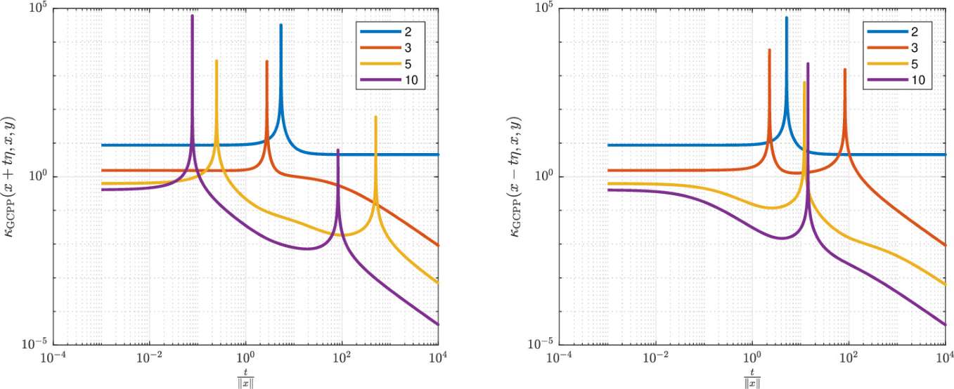
The next experiment illustrates how the condition number varies with the distance along a normal direction . We consider the setup from the previous paragraph. The projection of the point onto the image planes of the first cameras is . A random unit-norm normal vector in is chosen as described before. We investigate the sensitivity of the perturbed inputs for . The condition number is computed for these inputs for and for values of uniformly spaced between and . The results are shown in fig. 4. We have peaks for a fixed because . The two-camera system has only two singularities in the range . These figures illustrate the continuity of from corollary 14.
Up to about we observe that curvature hardly affects the condition number of the GCPP for the triangulation problem. Beyond this value, curvature plays the dominant role: both the singularities and the tapering off for high relative errors are caused by it. Moreover, the condition number decreases as the number of cameras increases. This indicates that the use of minimal problems [45] in computer vision could potentially introduce numerical instability.
Acknowledgements
The authors thank Nicolas Boumal for posing a question on unconstrained errors, which eventually started the project that led to this article. We are greatly indebted to Carlos Beltrán who meticulously studied the manuscript and asked pertinent questions about the theory. Furthermore, the authors would like to thank Peter Bürgisser for hosting the second author at TU Berlin in August 2019, and Joeri Van der Veken for fruitful suggestions and pointers to the literature.
We thank two anonymous reviewers whose remarks enticed us to immensely improve the presentation of our results, specifically in sections 1 and 3, and to include a discussion of computational aspects in section 8. We also thank the editor, Anthony So, for adeptly handling the reviewing process.
Appendix A Proofs of the technical results
We recall two classic results that we could not locate in modern references in differential geometry. A common theme in the three computational problems considered in sections 5, 4 and 6 is that they involve the projection from the normal bundle to the base of the bundle, the embedded submanifold . This projection is smooth [47, Corollary 10.36] and its derivative is characterized by the following classical result, which dates back at least to Weyl [67].
Proposition 21.
Let and . Then, where is as in eq. H.
A useful consequence is that it allows us to characterize when is singular.
Lemma 22.
Let , , and be as in eq. H. Then, is invertible if and only if .
Proof.
Let . Then, we have and , so that proposition 21 yields the equality of operators
| (10) |
On the one hand, if then the map is invertible. By multiplying with its inverse we get . As is an endomorphism on , which is the range of the left-hand side, the equality requires to be an automorphism, i.e., it is invertible.
On the other hand, if , there is some in the kernel of . Since , we must have . Consequently, applying both sides of eq. 10 to gives , which implies that is singular. This finishes the proof.
The next result follows almost directly from proposition 21 and appears several times as an independent statement in the literature. The earliest reference we could locate is Abatzoglou [1, Theorem 4.1], who presented it for embedded submanifolds of in a local coordinate chart.
Corollary 23.
Let be a Riemannian embedded submanifold. Then, there exists a tubular neighborhood of such that the projection map is a smooth submersion with derivative
where , , and is given by eq. H.
In the next subsections, proofs are supplied for the main results.
A.1 Proofs for section 4
Proof of lemma 3.
Recall that is a smooth map, so if its derivative is nonsingular at a point , then there exists an open neighborhood of where this property remains valid. Therefore, applying the inverse function theorem [47, Theorem 4.5] at , the fact that is invertible implies that there is a neighborhood of in and a neighborhood of in such that is diffeomorphic to (an open ball in) . Hence, is open in , and, hence, it is an open submanifold of dimension .
To show that is dense in , take any . Let . Then, because . By lemma 22, with if and only if is singular. This occurs only if equals one of the eigenvalues of the Weingarten map . Consequently, can be reached as the limit of a sequence , which is wholly contained in by taking outside of the discrete set.
Applying [47, Proposition 5.1], we can conclude that is even an embedded submanifold. This concludes the argument.
Proof of theorem 4.
Let be arbitrary. On , the coordinate projection has an invertible derivative. Consequently, by the inverse function theorem [47, Theorem 4.5] there exist open neighborhoods of and of such that has a smooth inverse function that we call . Its derivative is . Consider the smooth map , where is the coordinate projection. The CPP condition number at is . Since , we have that . Now it follows from lemmas 22 and 10 that . As the metrics on and are identical, . This concludes the first part.
The second part is lemma 22.
A.2 Proofs for section 5
Proof of lemma 7.
By corollary 23 the projection is a smooth map on . Let us denote the graph of this map by . It is a smooth embedded submanifold of dimension ; see, e.g., [47, Proposition 5.4]. Let , and be a nonzero tangent vector. Because of corollary 23 it satisfies . Hence, so that its kernel is trivial. It follows that . Since their dimensions match by lemma 2, is an open submanifold. As is embedded by lemma 3, is embedded as well by [47, Proposition 5.1]. Moreover, by construction, we have
The first part of the proof is concluded by observing that the proof of lemma 12 applies by replacing with and with .
Finally, we show that is dense in . Let with and be arbitrary. Then and . As is an open dense submanifold of , there exists a sequence such that . Consider with and chosen in such a way that the first component lies in the tubular neighborhood; this is possible as is an open submanifold of . Then, the limit of this sequence is . Q.E.D.
Proof of theorem 8.
For , let and . By eq. 2, Since , we know that is invertible. Moreover, by corollary 23 the derivative of the projection at is . Therefore,
For , we have with . By definition of , this entails that is not invertible, concluding the proof.
A.3 Proofs for section 6
Proof of lemma 12.
Combining 1 and 3, it is seen that is realized as the intersection of two smoothly embedded product manifolds:
Note that , by lemma 2, and , because and 1 stating that . Thus, it suffices to prove that the intersection is transversal [47, Theorem 6.30], because then would be an embedded submanifold of codimension .
Consider a point . Transversality means that we need to show
Fix an arbitrary . Then, it suffices to show there exist and such that It follows from propositions 21 and 22 that where and where . The tangent vectors , and can be chosen freely. Choosing and ; and and and yields . This concludes the first part of the proof.
It remains to prove is dense in . For this, we recall that
Let and let . Then, and . As is an open dense submanifold of by 1, there exists a sequence such that . Moreover, there exists a sequence with so that , because . Since is open dense in by lemma 3, only finitely many elements of the sequence are not in . We can pass to a subsequence . Now and moreover its limit is . Q.E.D.
Proof of theorem 13.
For a well-posed triple we obtain from eq. 2 that . We compute the right-hand side of this equation. The situation appears as follows:
We have in addition the projections and . With this we have
Taking derivatives we get
Since , the derivative is invertible, and so is also invertible. On other hand, since , the derivative is invertible. Altogether we see that is invertible, and that
The derivatives in the middle satisfy
while on the other hand This implies that the two linear maps on the right hand side in the previous equations are equal. Hence,
| (11) |
where we used eqs. 10 and 22. Taking spectral norms on both sides completes the proof for points in . Finally, for points outside the proof follows from the definition of combined with theorems 8 and 4.
A.4 Proofs for section 7
Proof of proposition 16.
Taking the derivative of the objective function at a point we see that the critical points satisfy for all . By the definition of , the derivative is surjective, which implies that . Therefore, the condition of being a critical point is equivalent to .
Proof of theorem 18.
By assumption . In particular, this implies , so that is invertible. By the inverse function theorem [47, Theorem 4.5], there is an open neighborhood of such that restricts to a diffeomorphism on
Let denote the inverse of on . Combining eqs. 10 and 22, the derivative of is given by and thus has constant rank on equal to . This implies that
has constant rank on equal to , by 1. Consequently, there is a smooth function with . The above showed that its derivative has constant rank equal to , so is a smooth submersion. By Proposition 4.28 of [47], is an open subset, so it is a submanifold of dimension . Similarly, the derivative at has maximal rank equal to , by definition of . Hence, is also a smooth submersion. After possibly passing to an open subset of , we can thus assume
are open submanifolds each of dimension and that
- (i)
is the global minimizer of the distance to on , and hence,
- (ii)
all lie on the same side of , considering the tangent space as an affine linear subspace of with base point .
Now let be a point in the neighborhood of . The restricted squared distance function that is minimized on is smooth. Its critical points satisfy
Since , the derivative of is invertible. Then, for all the image of is the whole tangent space . Consequently, the critical points must satisfy .
By construction, for every there is a unique so that , namely . This implies that is the unique critical point of the squared distance function restricted to .
It only remains to show that for all , the minimizer of is attained in the interior of . This entails that the unique critical point is also the unique global minimizer on . We show that there exists a such that restricting to the open ball of radius centered at in yields the desired result.
Here is the geometric setup for the rest of the proof, depicted in fig. 5: let and let be the minimizer for in the closure of . Then, is in the closure of by continuity of . Furthermore, let , where is the orthogonal projection onto the tangent space considered as an affine linear subspace of with base point .
The image of under is an open ball . The distance function measures the “height” of from the tangent space . Now, we can bound the distance from to as follows.
| (12) |
where the first bound is the triangle inequality, and where is the preimage of under the projection restricted to .
Now let be a point in the boundary of and, again, . We want to show that the distance is strictly larger than eq. 12. This would imply that local minimizer for is indeed contained in the interior of . We have
Note that . Hence we have the orthogonal decomposition
Plugging this into the above, we find
where .
Observe that points from to and likewise points from to . Therefore, because both point away from the manifold , which lies entirely on the side of by assumption (ii) above; see also fig. 5. Consequently, which implies
Note that is a continuous function with . Hence, as the maximum height tends to zero as well. Moreover, and are independent of . All this implies that we can choose sufficiently small so that
It follows that is lower bounded by eq. 12, so that the minimizer for must be contained in the interior of .
The foregoing shows that on , the map equals the nonlinear projection onto the manifold . Putting everything together, we obtain
the second equality following eq. 11. The condition number of this smooth map is given by eq. 2. Comparing with theorems 8 and 13 concludes the proof.
References
- [1] T. J. Abatzoglou, The minimum norm projection on manifolds in , Trans. Amer. Math. Soc., 243 (1978), pp. 115–122.
- [2] P.-A. Absil, R. Mahony, and R. Sepulchre, Optimization Algorithms on Matrix Manifolds, Princeton University Press, 2008.
- [3] P.-A. Absil, R. Mahony, and J. Trumpf, An extrinsic look at the Riemannian Hessian, in Geometric Science of Information, Lecture Notes in Computer Science, Springer, Berlin, Heidelberg, 2013.
- [4] D. Amelunxen and P. Bürgisser, A coordinate-free condition number for convex programming, SIAM J. Optim., 22 (2012), pp. 1029–1041.
- [5] J.-P. Aubin and H. Frankowska, Set-Valued Analysis, Birkhäuser Boston, reprint of the 1990 ed., 2009.
- [6] Z. Bai, J. Demmel, J. Dongarra, A. Ruhe, and H. van der Vorst, eds., Templates for the Solution of Algebraic Eigenvalue Problems: A Practical Guide, SIAM, Philadelphia, PA, 2000.
- [7] D. Bau and L. N. Trefethen, Numerical Linear Algebra, SIAM, 1997.
- [8] A. Belloni and R. M. Freund, A geometric analysis of Renegar’s condition number, and its interplay with conic curvature, Math. Program., Ser. A, 119 (2009), pp. 95–107.
- [9] T. Bendory, Y. C. Eldar, and N. Boumal, Non-convex phase retrieval from STFT measurements, IEEE Trans. Inform. Theory, 64 (2018), pp. 467–484.
- [10] L. Blum, F. Cucker, M. Shub, and S. Smale, Complexity and Real Computation, Springer-Verlag, New York, 1998.
- [11] N. Boumal, Riemannian trust regions with finite-difference Hessian approximations are globally convergent, in Geometric Science of Information, F. Nielsen and F. Barbaresco, eds., vol. 2, 2015, pp. 467–475.
- [12] , Nonconvex phase synchronization, SIAM J. Optim., 26 (2016), pp. 2355–2377.
- [13] , An introduction to optimization on smooth manifolds. Available online, 2020.
- [14] N. Boumal, B. Mishra, P.-A. Absil, and R. Sepulchre, Manopt, a Matlab toolbox for optimization on manifolds, J. Mach. Learn. Res., 15 (2014), pp. 1455–1459.
- [15] P. Breiding and N. Vannieuwenhoven, Convergence analysis of Riemannian Gauss–Newton methods and its connection with the geometric condition number, Appl. Math. Letters, 78 (2018), pp. 42–50.
- [16] , A Riemannian trust region method for the canonical tensor rank approximation problem, SIAM J. Optim., 28 (2018), pp. 2435–2465.
- [17] P. Bürgisser and F. Cucker, Condition: The Geometry of Numerical Algorithms, Springer, Heidelberg, 2013.
- [18] N. Chernov and H. Ma, Least squares fitting of quadratic curves and surfaces, in Computer Vision, S. Yoshida, ed., Nova Science Publishers, 2011.
- [19] D. Cheung and F. Cucker, A new condition number for linear programming, Math. Program., 91 (2001), pp. 163–174.
- [20] D. Cheung, F. Cucker, and J. Peña, A condition number for multifold conic systems, SIAM J. Optim., 19 (2008), pp. 261–280.
- [21] A. Coulibaly and J.-P. Crouzeix, Condition numbers and error bounds in convex programming, Math. Program., 116 (2009), pp. 79–113.
- [22] F. Cucker and J. Peña, A primal-dual algorithm for solving polyhedral conic systems with a finite-precision machine, SIAM J. Optim., 12 (2001), pp. 522–554.
- [23] C. Da Silva and F. J. Herrmann, Optimization on the hierarchical Tucker manifold – applications to tensor completion, Linear Algebra Appl., 481 (2015), pp. 131–173.
- [24] J. W. Demmel, The geometry of ill-conditioning, J. Complexity, 3 (1987), pp. 201–229.
- [25] , On condition numbers and the distance to the nearest ill-posed problem, Numer. Math., 51 (1987), pp. 251–289.
- [26] , Applied Numerical Linear Algebra, SIAM, 1997.
- [27] M. do Carmo, Riemannian Geometry, Birhäuser, 1993.
- [28] A. L. Dontchev and R. T. Rockafeller, Implicit Functions and Solution Mappings: A View From Varational Analysis, Springer Monographs in Mathematics, Springer, 2009.
- [29] J. Draisma, E. Horobet, G. Ottaviani, B. Sturmfels, and R. Thomas, The Euclidean distance degree of an algebraic variety, Found. Comput. Math., 16 (2016), pp. 99–149.
- [30] M. Epelman and R. M. Freund, Condition number complexity of an elementary algorithm for computing a reliable solution of a conic linear system, Math. Program., 88 (2000), pp. 451–485.
- [31] , A new condition measure, preconditioners, and relations between different measures of conditioning for conic linear systems, SIAM J. Optim., 12 (2002), pp. 627–655.
- [32] O. Faugeras and Q. Luong, The Geometry of Multiple Images, MIT Press, Cambridge, MA, 2001. The laws that govern the formation of multiple images of a scene and some of their applications, With contributions from Théo Papadopoulo.
- [33] F. Feppon and P. F. J. Lermusiaux, The extrinsic geometry of dynamical systems tracking nonlinear matrix projections, SIAM J. Matrix Anal. Appl., 40 (2019), pp. 814–844.
- [34] R. M. Freund and F. Ordóñez, On an extension of condition number theory to nonconic convex optimization, Math. Oper. Res., 30 (2005), pp. 173–194.
- [35] R. M. Freund and J. R. Vera, Condition-based complexity of convex opitimization in conic linear form via the ellipsoid algorithm, SIAM J. Optim., 10 (1999), pp. 155–176.
- [36] G. H. Golub and C. Van Loan, Matrix Computations, The John Hopkins University Press, 4 ed., 2013.
- [37] R. Hartley and A. Zisserman, Multiple View Geometry in Computer Vision, Cambridge University Press, Cambridge, second ed., 2003. With a foreword by Olivier Faugeras.
- [38] G. Heidel and V. Schulz, A Riemannian trust-region method for low-rank tensor completion, Numer. Linear Algebra Appl., 25 (2018).
- [39] A. Heyden and K. Åström, Algebraic properties of multilinear constraints, Math. Meth. Appl. Sci., 20 (1997), pp. 1135–1162.
- [40] N. Higham, Accuracy and Stability of Numerical Algorithms, SIAM, Philadelphia, PA, 1996.
- [41] M. W. Hirsch, Differential Topology, no. 33 in Graduate Text in Mathematics, Springer-Verlag, 1976.
- [42] S. Holtz, T. Rohwedder, and R. Schneider, On manifolds of tensors of fixed TT-rank, Numer. Math., 120 (2012), pp. 701–731.
- [43] J. Humpherys, T. J. Jarvis, and E. J. Evans, Foundations of Applied Mathematics, SIAM, 2017.
- [44] D. Kressner, M. Steinlechner, and B. Vandereycken, Low-rank tensor completion by Riemannian optimization, BIT Numer. Math., 54 (2014), pp. 447–468.
- [45] Z. Kúkelová, Algebraic Methods in Computer Vision, PhD thesis, Czech Technical University in Prague, 2013.
- [46] J. M. Lee, Riemannian Manifolds: Introduction to Curvature, Springer-Verlag, 1997.
- [47] J. M. Lee, Introduction to Smooth Manifolds, Springer, New York, USA, 2 ed., 2013.
- [48] Y. Liu and W. Wang, A revisit to least squares orthogonal distance fitting of parametric curves and surfaces, in Advances in Geometric Modeling and Processing, F. Chen and B. Juttler, eds., Lecture Notes in Computer Science, 2008.
- [49] MATLAB, R2017b. Natick, Massachusetts, 2017.
- [50] S. Maybank, Theory of Reconstruction from Image Motion, vol. 28 of Springer Series in Information Sciences, Springer-Verlag, Berlin, 1993.
- [51] B. O’Neill, Semi-Riemannian Geometry, Academic Press, 1983.
- [52] , Elementary Differential Geometry, Elsevier, revised second edition ed., 2001.
- [53] J. Peña and V. Roshchina, A data-independent distance to infeasibility for linear conic systems, SIAM J. Optim., 30 (2020), pp. 1049–1066.
- [54] P. Petersen, Riemannian Geometry, vol. 171 of Graduate Texts in Mathematics, Springer, New York, second ed., 2006.
- [55] I. R. Porteous, The normal singularities of a submanifold, J. Differ. Geom., 5 (1971).
- [56] J. Renegar, Incorporating condition measures into the complexity theory of linear programming, SIAM J. Optim., 5 (1995), pp. 506–524.
- [57] , Linear programming, complexity theory and elementary functional analysis, Math. Program., 70 (1995), pp. 279–351.
- [58] J. R. Rice, A theory of condition, SIAM J. Numer. Anal., 3 (1966), pp. 287–310.
- [59] M. Spivak, A Comprehensive Introduction to Differential Geometry, vol. 2, Publish or Perish, Inc., 1999.
- [60] M. Steinlechner, Riemannian optimization for high-dimensional tensor completion, SIAM J. Sci. Comput., 38 (2016), pp. S461–S484.
- [61] A. Sung-Joon, Geometric fitting of parametric curves and surfaces, J. Inf. Process. Syst., 4 (2008), pp. 153–158.
- [62] R. Thom, Sur la theorie des enveloppes, J. Math. Pures Appl., 41 (1962), pp. 177–192.
- [63] B. Vandereycken, Low-rank matrix completion by Riemannian optimization, SIAM J. Optim., 23 (2013), pp. 1214–1236.
- [64] J. R. Vera, Ill-posedness and the complexity of deciding existence of solutions to linear programs, SIAM J. Optim., 6 (1996), pp. 549–569.
- [65] , Geometric measures of convex sets and bounds on problem sensitivity and robustness for conic linear optimization, Math. Program., 147 (2014), pp. 47–79.
- [66] Visual Geometry Group, University of Oxford, Model house data set, Last accessed 28 september 2020. Access online at https://www.robots.ox.ac.uk/~vgg/data/data-mview.html.
- [67] H. Weyl, On the volume of tubes, Amer. J. Math., 2 (1939), pp. 461–472.
- [68] J. H. Wilkinson, Rounding Errors in Algebraic Processes, Prentice-Hall, Englewood Cliffs, New Jersey, 1963.
- [69] , The Algebraic Eigenvalue Problem, Oxford University Press, Amen House, London, United Kingdom, 1965.
- [70] H. Woźniakowski, Numerical stability for solving nonlinear equations, Numer. Math., 27 (1976/77), pp. 373–390.