The Stroke Correspondence Problem, Revisited
Abstract
We revisit the stroke correspondence problem [13, 14]. We optimize this algorithm by 1) evaluating suitable preprocessing (normalization) methods 2) extending the algorithm with an additional distance measure to handle Hiragana, Katakana and Kanji characters with a low number of strokes and c) simplify the stroke linking algorithms. Our contributions are implemented in the free, open-source library ctegaki and in the demo-tool jtegaki.
1 Introduction
Revisiting the stroke correspondence problem is motivated by developing a robust, freely available, open-source Japanese on-line handwriting recognition engine, especially considering the current advance of touch-driven mobile devices. For handwriting recognition, learning based methods have largely replaced approaches based on template matching. Popular methods are directional feature extraction [2] and classification by MQDF [3], or approaches based on neural networks [7]. In order to a achieve satisfactory performance, learning based methods however require lots of training samples for each character [9]. Several large databases with training samples exist, cf. [10, 8, 6], or the JEITA-HP database. To the author’s best knowledge, none of them is available under a free license that would permit use in free/libre open-source software. On the other hand, generating such a database from scratch is no easy task; for example [8] write – despite being full-time academic researchers – that they spent 4 years compiling […] databases, and such a monumental task is difficult to achieve within an open-source project. This is probably one main reason why none of the above mentioned high-performing recognition approaches have been implemented and released as open source.
It is very important for a recognition engine to be able to cope with stroke-order and stroke-number variations. While in theory the number and the order of strokes is uniquely defined for each kanji character, in practice they vary widely w.r.t. individual writing styles. Native speakers for example tend to combine several strokes into one in order to write faster (cursive style), and foreign leaners of the language often do not know the correct stroke order. A recognition algorithm must thus be able to recognize kanji independent on stroke-order and stroke-number.
The only two open-source Japanese online character recognition engines the author is aware of - zinnia11 1 http://www.zinnia.sourceforge.net and wagomu22 2 http://tegaki.org use learning based approaches and employ a rather small training data set of one sample per character. Therefore they cannot cope with stroke-number or stroke-order variations very well.
In this paper, a simple approach of directly linking a written character to a reference template pattern [14] is revisited. Recognition is then performed by directly comparing the reference template with the input pattern, and the ability to cope with stroke-order and stroke-number variations is inherent in the comparison. Such an approach has the big advantage, that no training data is needed, and one reference template for each character suffices. [11] used a similar approach using directional features for reference templates, resulting in a very high recognition rate. This comes at the cost of stroke-number free recognition, and a sophisticated but complex data-structure and search algorithm. In this paper the original approach [14] is extended by
- 1.
evaluating which image normalization techniques is the overall performance.
- 2.
introducing a distance measure using directional features akin to [11]. This increases recognition performance of Hiragana, Katakana and Kanji with a low number of strokes.
- 3.
Last, a simple-to-implement yet well-performing stroke linking algorithm is introduced, replacing the two complementing algorithms defined by [14].
All techniques have been implemented in the open-source library ctegaki, which is available under a free BSD-style license at
https://github.com/asdfjkl/ctegaki-lib
Moreover a JavaScript-based demo application is available at
https://asdfjkl.github.io/kanjicanvas
This paper is structured as follows. In Section 2 the stroke correspondence problem is reviewed and distance measures are introduced. Suitable normalization methods are discussed in Section 3. Two complementing algorithms were used by [14] for stroke linking. A new algorithm is introduced in Section 4. The overall recognition algorithm is presented in Section 5. The effect of various normalization algorithms, the newly introduced directional distance measure, and the new stroke linking algorithm, as well as overall performance compared to the open source recognition library Zinnia, is empirically evaluated in Section 6. Last, the presentation is concluded in Section 7.
2 The Stroke Correspondence Problem
A kanji character is defined as a set of strokes . This set is ordered w.r.t. the index of the strokes which represent the order in which the strokes were drawn. A strokes is a set of points , again ordered by their indices. A point is a 2D-coordinate. Let be a kanji with strokes , and be a kanji with strokes . In the following we assume w.l.o.g. . Given two sets of strokes and , a stroke distance function is a function .
Given two kanji with the same number of strokes and a stroke distance function, the stroke correspondence problem is the optimization problem to find a mapping between the strokes that minimizes the overall distance.
Definition 1 ( Stroke Correspondence Problem)
Let and be two kanji both of length , and a stroke distance function. The stroke correspondence problem is the problem to find a bijective function , that minimizes .
The general idea for recognition is to define one template for each kanji. Given an input kanji that should be recognized, a minimizing function is computed for each pair of the input kanji and one template. Then the overall distance between the input kanji and the template is calculated w.r.t. the minimizing function, and the result of the recognition is the template with the smallest distance. Since the minimizing function does not incorporate any stroke order, this recognition approach is completely independent of the stroke order.
Two problems arise with this approach. First, given a kanji and a template with strokes, the cost of finding a minimizing function is in . Fast approximation algorithms for are subject of Section 4. Second, the definition can only cope with input kanji and templates that have the same number of strokes. To deal with kanji of arbitrary numbers of strokes, the definition is extended. Given two strokes and , the concatenated stroke of and is defined as the union , where the order of points is extended such that all points of are smaller than those of , i.e. the points of are appended to . Concatenation is extended in the obvious way to arbitrary numbers of strokes. Given , the concatenation of all strokes is denoted by . In the next definition, only surjectivity is required for :
Definition 2 ( Stroke Correspondence Problem)
Suppose two kanji and are given, and let be a stroke distance function. The stroke correspondence problem is the problem to find an surjective function , that minimizes
This optimization problem depends on the definition of the stroke distance function. These are subject of the next section.
2.1 Stroke Distance Functions
Three distance functions were originally introduced by [14].
Definition 3 (Endpoint Distance)
Suppose two strokes and are given. The endpoint distance is defined as
In the original definition, the calculation used division by some constant. This is omitted here. Since the computation of the endpoint distance is quite efficient, it can be used for a quick coarse classification to find suitable candidates. For fine classification, the next two distance measures were introduced. In the next definition, it is assumed that . Hence, division results in a real number.
Definition 4 (Initial Stroke Distance)
Suppose two strokes and . Let . The initial stroke distance is defined as
The next distance measure is the most precise one.
Definition 5 (Whole-Whole Stroke Distance)
Suppose and . Let . The whole-whole stroke distance is defined as
Here , integer division is used for the calculation of , and the division for is in .
None of these stroke distances emphasize the actual stroke direction. [11] used directional features for stroke order independent (but not stroke number independent) recognition. Directional features are especially important when recognizing kanji with low number of strokes, or hiragana and katakana characters. Consider for example
しand
乙. If the stroke of these characters is represented by only a few points, all above mentioned stroke distances will result in a low overall distance, and hence distinguishing these characters is difficult. On the other hand, the two characters have very distinct directional features. This motivates the next definition, which is new compared to those introduced by [14].
Definition 6 (Directional Stroke Distance)
Let and , and let . The directional stroke distance is defined as
where and is computed with integer division, whereas the in is division in .
3 Normalization Methods
Image Normalization is an important pre-processing step in character recognition. Given an image with height and width (i.e. a bounding box around the drawn character), image normalization projects this image to a an image with pre-defined height and width . Throughout this section, we will consider a kanji as binary image (function) .
Definition 7 (Linear Normalization)
Let be an input coordinate. Supposed and are the height and width of the input image, and and the height and width of the normalized image. The transformed coordinate is defined as: and .
In the recognition approach of this paper, linear normalization is used only when the width and height of a character are very different. It then makes sense to keep the aspect ratio, and multiply only by the minimum of and (cf. Section 5).
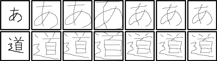
Moment normalization was originally formulated by [1], but here the simplified variant introduced by [5] is used. Recall that given an image (function) , (raw) image moments are defined as . Components of the centroid are and , and central moments of the image are defined as .
Definition 8 (Moment Normalization)
Let be an input coordinate. Supposed and are the height and width of the input image, and and the heigth and width of the normalized image. Let and . Distinct from other normalization methods, the bounding box of the input image is first reset to The transformed coordinate is defined as:
The effect on normalization techniques has been studied before especially in the context of directional feature extraction [4, 5]. As can be seen in the latter, the introduction of advanced pseudo 2D normalization techniques improves recognition rates. However non-linear normalization [15, 12] is a simple and fast technique that achieves a significant improvement over no or linear-normalization. The investigation is thus restricted here to the non-linear normalization techniques introduced by [15]. The next two methods rely on feature projection functions and .
Definition 9 (Dot Density Equalization)
Let and be given constants, and let denote the input image, and the height and width of the input and normalized image. The projection functions are defined as: and The normalized image is defined as:
| (1) |
Line density equalization works similar as dot density equalization, but employs a more advanced density projection.
Definition 10 (Line Density Equalization)
To define feature projections, first four types of edges are defined for a given point . Below denotes the inverted pixel .
Note that there is a case where is not defined. Based on these four types of edges, horizontal and vertical line intervals are defined. Let denote width and height of the input image. is defined as 1) , if all are not defined, 2) , if only are not defined, 3) , if only are not defined, 4) , if only are not defined, 5) , if only is not defined, 6) , if only is not defined, and finally , otherwise.
The line interval for the vertical direction is defined analogously, where is taken instead of , and edge definitions are changed w.r.t. vertical directions. Line densities are defined as: if + , and , otherwise. Projection function are defined by
| (2) |
The actual mapping coordinates are then obtained by inserting the projection functions of in equation of Definition 9.
4 Stroke Linking Algorithms
The goal of a stroke linking algorithm is to find a (surjective) mapping function that meets the condition of Definition 2. In the original paper by [13], the following approach was proposed: First, find a mapping from out strokes of kanji to the strokes of kanji . Second, if , the remaining strokes of are then concatenated with their preceding or following strokes. For the first step they propose two complementing algorithms, excessive mapping dissolution (EMD) and deficient mapping dissolution (DMD). The motivation to introduce two algorithms is shown in Figure 2. Considering a distance measure that simply computes the manhattan distance of two points, two mapping cases are depicted. For one case, EMD succeeds to find the optimal mapping whereas DMD fails, and in the other case, the reverse is true.

Both from the perspective of run-time and implementation complexity, it is desirable to have only one single algorithm. A simple approach is just to use a greedy strategy, where, iterating over all strokes from , given stroke from , an unassigned stroke out of the stroke of is chosen for which the distance is minimal. Manual inspection of such computed stroke maps revealed that in practice usually only very few excessive local minima cause a mapping that does not yield a global minimum. The typical cause of such local minima are strokes of very short length, which yield a very short local minimum with almost every nearby stroke, such as the first two strokes of
字. This is the motivation to introduce the iterative improvement algorithm. Technically this is one algorithm, but for the ease of presentation, the greedy initialization part as described above is shown separately as Algorithm 1, whereas the remaining part of the algorithm is shown as Algorithm 2. Algorithm 2 loops a fixed set of times over the initialized stroke map, and in each loop switches the current assignment to another assigned stroke (line 9 to 17), or to another unassigned stroke (line 18 to 25), if the resulting distance can be improved by switching.
Two examples are given in the style of [13]. Originally they illustrated the complementary nature of EMD and DMD, and here it is shown how iterative improvement succeeds in both cases. For the ease of illustration, the examples consider strokes that contain only one point. Also for simplicity, the distance between two strokes is defined as the manhattan distance between the corresponding two points, and for that the example is slightly modified compared to the original example.
Example 1
Consider the left example of Figure 2. Greedy initialization results in the following stroke map: Here the index of the array denotes a stroke of , and the content is a stroke of : Next, Algorithm 2 iterates over strokes of , and tests whether switching strokes decreases overall cost. First:
Since , nothing is changed. The next comparison is:
Since , the assignments are switched and result in It is not difficult to see that one additional iteration will result in the optimal assignment .
Example 2
Consider the right example of Figure 2. Greedy initialization results in: The first step of iterative improvement compares
Since , the optimal map is immediately found.
5 Recognition Algorithm
Putting all previous sections together and taking into account the original approach by [13], the algorithm presented below is used for recognition. The input is an unknown kanji . It is assumed that templates exist, where one templates corresponds to one unique kanji character.
5.1 Recognition Algorithm
Interpolation: The input kanji’s resolution might not be dense enough. For example for a straight line, only the input and end coordinate might be specified. To get a higher resolution, intermediate points between each given point and its successor are computed using Bresenham’s line algorithm.
Normalization: The input kanji is normalized to an area of 256x256 pixels. To avoid excessive distortions for kanji characters that have a large difference w.r.t. length and heigth (such as e.g.
一), linear normalization is used whenever 3*heigth width or vice versa. Otherwise one of the following is used: linear normalization, moment normalization, normalization by line density equalization, or normalization by dot density equalization with or .
Interpolation: Normalization can decrease the resolution, and thus again intermediate points are interpolated using Bresenham’s line algorithm.
Feature Point Extraction: For each stroke, feature points are extracted. The initial and end point of a stroke are always extracted. Intermediate points are extracted in a way such that the euclidian distance between two consecutive points is close to a fixed global value. In the implementation, a fixed value of 20.0 is used. The result of this step is a kanji with the same number of strokes as the input kanji, but each stroke has a much lower number of (extracted feature) points.
Coarse Classification: It is assumed that each template has been preprocessed in the same way as described above. Next coarse classification finds a predefined set (in our implementation: 100) of candidates, in the following way:
For each template , a stroke map of and is computed. First, the stroke map is initialized by Algorithm 1, and improved in steps by Algorithm 2. In both cases endpoint distance is used. If both and have the same number of strokes, the overall endpoint distance between and is calculated using the computed stroke map. Otherwise, the stroke map is completed in the following way:
- 1.
Let be the smallest where . Then all strokes are mapped to .
- 2.
Let be the largest such that and all have . Then all strokes are mapped to .
- 3.
Suppose that there are with , , , and for all with there is . A split point can be chosen among all in the following way: is set to for all , and is set to for all . The split point is chosen in a way such that the overall computed distance is minimal.
The result of the coarse classification are those 100 templates, that yield the smallest overall stroke correspondence between and the template with the above computed stroke map using the endpoint distance measure.
Fine Classification: During fine classification, ten templates are chosen among those 100 that are selected by coarse classification. First a stroke map between and each template is computed using Algorithm 1 and 2 with the initial distance measure. If template and do not possess the same number of strokes, the stroke map is completed as in coarse classification. However instead of using the endpoint distance measure, the following approach is used:
- 1.
If the input has less than a predefined number of strokes, then the stroke map is completed using the directional distance measure.
- 2.
Otherwise, the whole-whole distance measure is used. The predefined number is chosen empirically, cf. Table 2.
Finally a weight for each template is computed. Let . Below, is written for Using the above computed stroke map, the following weight is computed:
Here, for two strokes containing and points, , if or resulted from concatenation, and , otherwise. The result of the fine classification are those ten templates, that yield the lowest weights .
| Linear | Moment | DotDensity | DotDensity | DotDensity | LineDensity | |
|---|---|---|---|---|---|---|
| Kanji (79) | ||||||
| Top 1 | 63 | 62 | 61 | 62 | 60 | 60 |
| Top 5 | 72 | 73 | 70 | 71 | 72 | 70 |
| Top 10 | 74 | 75 | 73 | 73 | 74 | 71 |
| Hiragana (46) | ||||||
| Top 1 | 30 | 37 | 35 | 33 | 29 | 26 |
| Top 5 | 43 | 44 | 45 | 45 | 45 | 49 |
| Top 10 | 45 | 45 | 45 | 45 | 45 | 32 |
| Katakana (46) | ||||||
| Top 1 | 32 | 41 | 32 | 33 | 32 | 35 |
| Top 5 | 46 | 46 | 46 | 46 | 46 | 46 |
| Top 10 | 46 | 46 | 46 | 46 | 46 | 46 |
| Stroke Linking Algorithm | ||||||
|---|---|---|---|---|---|---|
| Kanji (79) | Timing (ms) | |||||
| Top1 | Top5 | Top10 | Min. | Max. | Avg. | |
| Original [13] | ||||||
| DMD | 62 | 73 | 74 | 5 | 207 | 16 |
| EMD | 59 | 68 | 71 | 4 | 135 | 13 |
| combined | 62 | 73 | 75 | 7 | 294 | 24 |
| -Iterative Improvement | ||||||
| (1,1) | 59 | 68 | 73 | 4 | 137 | 16 |
| (1,2) | 62 | 73 | 75 | 4 | 136 | 15 |
| (1,3) | 62 | 73 | 75 | 4 | 142 | 18 |
| (2,1) | 59 | 69 | 73 | 5 | 148 | 19 |
| (2,2) | 62 | 73 | 75 | 5 | 171 | 21 |
| (2,3) | 62 | 73 | 75 | 5 | 171 | 22 |
| (3,1) | 59 | 69 | 73 | 6 | 168 | 25 |
| (3,2) | 62 | 73 | 75 | 6 | 168 | 26 |
| (3,3) | 62 | 73 | 75 | 6 | 176 | 28 |
| Directional vs. Whole-Whole | |||||||
| zinnia | S=0 | S=1 | S=2 | S=3 | S=4 | S=5 | |
| Kanji (79) | |||||||
| Top 1 | 36 | 63 | 63 | 63 | 62 | 61 | 61 |
| Top 5 | 46 | 76 | 76 | 76 | 76 | 76 | 74 |
| Top 10 | 47 | 76 | 76 | 76 | 76 | 76 | 74 |
| Hiragana (46) | |||||||
| Top 1 | 27 | 35 | 35 | 34 | 33 | 33 | 33 |
| Top 5 | 35 | 42 | 42 | 43 | 43 | 45 | 45 |
| Top 10 | 37 | 44 | 44 | 46 | 46 | 46 | 46 |
| Katakana (46) | |||||||
| Top 1 | 34 | 37 | 37 | 39 | 44 | 46 | 46 |
| Top 5 | 41 | 45 | 45 | 45 | 46 | 46 | 46 |
| Top 10 | 42 | 45 | 45 | 45 | 46 | 46 | 46 |
6 Experiments
To evaluate the implemented recognition algorithm, 2264 templates were created. This set contains one template each for all jouyou kanji (kanji characters for every day use defined by the Japanese Ministry of Education), as well as one template each for all hiragana and katakana characters. To test the recognition performance, a test set of 79 characters was prepared. These include 49 characters from the distribution of Tegaki-Lab33 3 https://github.com/cburgmer/tegaki/tree/master/tegaki-lab, and the remaining characters include various characters that were deliberately written in a sloppy semi-cursive style with stroke concatenations on the one hand, and on the other hand with mistakes in stroke order and style that a typical foreign learner of the language would make. Normalization experiments and stroke linking experiments were conducted with a graphical prototype application written in Java. The recognition part was then ported to pure C, and the remaining experiments were done with that C-Library. All tests were run on an Intel Core i5 @ 2.5 Ghz with 8 GB RAM running Mac OS X 10.9.4.
Normalization Methods
For normalization, the recognition method described in Section 3 was used. For fine classification, only the initial stroke distance (as the input to Algorithm 1 and 2) as well as whole-whole stroke distance (for computation of the weights) was used. The directional stroke distance was not utilized. The results are depicted in Table 1. Whereas in statistical classification using directional features non-linear normalization is known to significantly improve recognition performance [2], contrary to what was conjectured by [13], the recognition performance is actually not increased by non-linear normalization methods. In fact for kanji characters, simple linear normalization outperforms all non-linear normalization methods. On the other hand, when it comes to hiragana and katakana characters, which are more similar in style to western handwriting, it can be seen that moment normalization significantly outperforms all other methods. The performance of non-linear normalization methods can be explained by the fact that they put more emphasis on and unify directional features at the cost of introducing distortions. Statistical classification methods that depend on directional features are not affected by this, but the distortions cause misrecognition for template matching. Thus in the implemented library and in further experiments, moment normalization was used due to its good overall performance.
6.1 Stroke Linking Algorithms
Next the performance of -iterative improvement was tested. Fine classification was conducted with the same distance measures as in the previous section. However computation of the stroke map was done once with the algorithms by [13], i.e. only DMD, only EMD, and combined, and once with iterative improvement. The results are depicted in Table 2. Note that each combination is run twice, once for the computation of a stroke map during coarse classification and fine classification each. The first (second) number in brackets for iterative improvement denote what the value was set to during coarse (fine) classification.
As can be seen, DMD itself performs quite well but fails in some examples. EMD itself performs not very well, but complements DMD and improves overall recognition performance. As for -iterative improvement, a combination of suffices to recognize all those characters that can be recognized by DMD & EMD. But the average recognition time compared to the combination of DMD & EMD is improved by -iterative improvement by more than one third, and for particular time intensive characters with a large number of strokes, the maximal recognition time is decreased by more than 50 percent.
6.2 Overall Performance and Directional Stroke Distance
Last, the recognition part of the Java prototype was ported to C. Due to different rounding results, especially w.r.t. to feature point extraction, slightly different recognition results compared to the Java prototype were obtained. Coarse classification was run with endpoint distance and iterative improvement, and fine classification was run also with iterative improvement but initial distance to get an strokemap, and the the stroke map was completed either using directional distance if the input character has less than strokes, or by using using directional distance, otherwise. Also, the performance was compared to the open-source online Japanese handwriting recognition library Zinnia, which uses a learning based approach with support vector machines. Zinnia was trained with exactly the same templates, and the same test data was supplied for recognition. The results are depicted in Table 3. As can be seen, a larger factor of improves recognition for hiragana and katakana characters, since they can be better distinguished using directional features. On the other hand, recognition performance of kanji characters decreases slightly. Nevertheless, the presented template based matching approach significantly outperforms the learning based approach of Zinnia, which performs poorly due to having only one training sample per character.
7 Conclusion and Future Work
Ideally, a large set of training samples for Japanese on-line character recognition would be available under an open-source (BSD-style) license, and a learning based approach could then be used for open-source Japanese on-line handwriting recognition. Since this is not the case, and such a database is unlikely to appear in near future due to the significant cost and logistics required, the focus here was on a template based matching approach. By empirically studying different normalization methods, extending the original approach by a new distance measure, and simplifying and unifying the underlying stroke linking algorithms, a fast and highly accurate implementation was achieved. Moreover it could be shown that in the present test set, the template based approach significantly outperforms competing learning-based implementations.
References
- [1] Casey, R.: Moment normalization of handprinted characters. IBM Journal of Research and Development 14(5), 548–557 (Sep 1970)
- [2] Kawamura, A., Yura, K., Hayama, T., Hidai, Y., Minamikawa, T., Tanaka, A., Masuda, S.: Online recognition of freely handwritten Japanese characters using directional feature densities. In: Pattern Recognition, 1992. Vol.II. Conference B: Pattern Recognition Methodology and Systems, Proceedings., 11th IAPR International Conference on. pp. 183–186 (Aug 1992)
- [3] Kimura, F., Takashina, K., Tsuruoka, S., Miyake, Y.: Modified quadratic discriminant functions and the application to Chinese character recognition. Pattern Analysis and Machine Intelligence, IEEE Transactions on PAMI-9(1), 149–153 (Jan 1987)
- [4] Lee, S.W., Park, J.S.: Nonlinear shape normalization methods for the recognition of large-set handwritten characters. Pattern Recognition 27(7), 895 – 902 (1994)
- [5] Liu, C.L., Marukawa, K.: Pseudo two-dimensional shape normalization methods for handwritten Chinese character recognition. Pattern Recognition 38(12), 2242 – 2255 (2005)
- [6] Liu, C.L., Yin, F., Wang, D.H., Wang, Q.F.: CASIA online and offline Chinese handwriting databases. In: Proceedings of the 2011 International Conference on Document Analysis and Recognition. pp. 37–41. ICDAR ’11 (2011)
- [7] Liu, C.L., Yin, F., Wang, Q.F., Wang, D.H.: ICDAR 2011 Chinese handwriting recognition competition. In: Document Analysis and Recognition (ICDAR), 2011 International Conference on. pp. 1464–1469 (Sept 2011)
- [8] Nakagawa, M., Matsumoto, K.: Collection of on-line handwritten Japanese character pattern databases and their analyses. Int. J. Doc. Anal. Recognit. 7(1), 69–81 (2004)
- [9] Rowley, H., Goyal, M., Bennett, J.: The effect of large training set sizes on online Japanese Kanji and English cursive recognizers. In: Frontiers in Handwriting Recognition, 2002. Proceedings. Eighth International Workshop on. pp. 36–40 (2002)
- [10] Saito, T., Yamada, H., Yamomoto, K.: On the data base ETL9 of handprinted characters in JIS chinese characters and its analysis (in japanese). Transactions IECE Japan J68(D(4)), 757–764 (1985)
- [11] Shin, J.p.: Optimal stroke-correspondence search method for on-line character recognition. Pattern Recogn. Lett. 23(5), 601–608 (Mar 2002)
- [12] Tsukumo, J., Tanaka, H.: Classification of handprinted Chinese characters using nonlinear normalization and correlation methods. In: Pattern Recognition, 1988., 9th International Conference on. pp. 168–171 vol.1 (Nov 1988)
- [13] Wakahara, T., Suzuki, A., Nakajima, N., Miyahara, S., Odaka, K.: On-line cursive kanji character recognition as stroke correspondence problem. In: Document Analysis and Recognition, 1995., Proceedings of the Third International Conference on. vol. 2, pp. 1059–1064 (Aug 1995)
- [14] Wakahara, T., Suzuki, A., Nakajima, N., Miyahara, S., Odaka, K.: Stroke-number and stroke-order free on-line kanji character recognition as one-to-one stroke correspondence problem. IEICE Transactions on Information and Systems E79-D(5), 529–534 (1996)
- [15] Yamada, H., Yamamoto, K., Saito, T.: A nonlinear normalization method for handprinted kanji character recognition—line density equalization. Pattern Recognition 23(9), 1023 – 1029 (1990)