跳到论文正文
W Papers独立论文阅读器 arXiv:1909.11941 论文正文 计算阅读时间 · 0%
引用这篇论文根据当前论文元数据生成,正式投稿前建议核对。


License: arXiv.org perpetual non-exclusive license
arXiv:1909.11941v2 [hep-ph] 16 Mar 2020

Fate of false vacuum in singlet-doublet fermion extension model with RG improved effective action

Yu Cheng Email: chengyu@mail.ecust.edu.cn Affiliation:  Institute of Modern Physics, School of Sciences,
East China University of Science and Technology, 130 Meilong Road, Shanghai 200237, P. R. China
   Wei Liao Email: liaow@ecust.edu.cn Affiliation:  Institute of Modern Physics, School of Sciences,
East China University of Science and Technology, 130 Meilong Road, Shanghai 200237, P. R. China
Abstract

We study the effective potential and the Renormalization Group(RG) improvement to the effective potential of Higgs boson in a singlet-doublet fermion dark matter extension of the Standard Model(SM), and in general singlet-doublet fermion extension models with several copies of doublet fermions or singlet fermions. We study the stability of the electroweak vacuum with the RG improved effective potential in these models beyond the SM. We study the decay of the electroweak vacuum using the RG improved effective potential in these models beyond the SM. In this study we consider the quantum correction to the kinetic term in the effective action and consider the RG improvement of the kinetic term. Combining all these effects, we find that the decay rate of the false vacuum is slightly changed when calculated using the RG improved effective action in the singlet-doublet fermion dark matter model. In general singlet-doublet fermion extension models, we find that the presence of several copies of doublet fermions can make the electroweak vacuum stable if the new Yukawa couplings are not large. If the new Yukawa couplings are large, the electroweak vacuum can be turned into metastable or unstable again by the presence of extra fermions.

I Introduction

Quantum contribution to the effective potential is important to understand the properties of the scalar field, e.g. the property of the ground-state and the behavior at large energy scale. For example, radiative correction can make a vacuum unstable and trigger spontaneous symmetry breaking Coleman:1973jx. The RG improved effective potential, which re-sums contributions of large logarithms, is important to understand the behavior of effective potential at large energy scale. For example, the RG-improved effective potential is crucial in reducing the dependence on the renormalization scale when calculating quantities related with physical parameters  Ford:1992mv; Bando et.al.; Casas:1994qy.

It is well known that a false vacuum can decay via tunneling  Langer; Coleman:1977py; Callan:1977pt and become unstable. In the SM, the Higgs quartic self-coupling can become negative at an energy scale around 101010^{10} GeV. This makes the electroweak(EW) vacuum unstable. The decay rate of the EW vacuum can be calculated using an approximate bounce solution of the Higgs potential with a negative Higgs quartic coupling  Isidori:2001bm; Chigusa:2018uuj; Chigusa:2017dux. Calculation of vacuum decay using RG improved effective potential in the SM does not give much difference, because the bounce solution is dominated by behavior at high energy scale and the RG-improved effective potential in the SM at high energy scale is accidentally close to the Higgs potential with running quartic coupling Degrassi:2012ry.

In extension of the SM, the situation can be quite different. The RG improved effective potential is possible to be very different from the potential using a running Higgs quartic coupling. As an example, we consider a singlet-doublet fermion dark matter(SDFDM) extension of the SM. We show that the RG improved effective potential can be quite different from the tree-level potential aided with running Higgs quartic coupling. Then we study the vacuum stability in this extension of SM. We study the false vacuum decay using RG improved effective potential in this SDFDM model. We also study the quantum contribution to the kinetic term in the effective action in this model beyond the SM and consider the RG improvement of the kinetic term. After taking all these effects into account we find that the false vacuum decay rate is just slightly changed using the RG improved effective action in the SDFDM model, although the RG effective potential is significantly different from the tree-level form of the Higgs potential with running quartic self-coupling. We also perform these analyses in general singlet-doublet fermion extension models in which several copies of singlet fermions or several copies of doublet fermions are considered. We find that the presence of several extra doublet fermions can make the EW vacuum stable if the new Yukawa couplings are not large.

The article is organized as follows. In section II, we first briefly review the SDFDM model. We study the threshold effect caused by the extra fermions in this model beyond the SM and study the running of the Higgs quartic coupling in this model. Then we study the effective potential and the RG improved effective potential in this model. In Section III we study the vacuum stability in SDFDM model. We calculate the renormalization of the kinetic term in the effective action in the SM and in SDFDM model. We study the RG improvement of the kinetic term and calculate the decay rate of the false vacuum. In Section IV, we do the analysis in general singlet-doublet fermion extension model. Details of calculation are summarized in Appendix A, B, C, and D. We summarize in conclusion.

II Effective potential and RG improved effective potential in SDFDM model

II.1 The SDFDM model

In addition to the SM fields, the SDFDM model has SU⁡(2)\mathrm{SU}(2) doublet fermions ψL,R=(ψL,R0,ψL,R−)T\psi_{L,R}=\left(\psi_{L,R}^{0},\psi_{L,R}^{-}\right)^{T} with Y = -1/2 and singlet fermions SL,RS_{L,R}. Here, LL (RR) refers to the left(right) chirality. As a singlet, SS can be either Dirac type or Majorana type fermion Cohen:2011ec; Freitas:2015hsa. In this model, the neutral fermion can be a dark matter candidate. The vacuum properties of SDFDM model with a Majorana type mass have been discussed in Wang:2018lhk. In this article we work on the Dirac type mass Yaguna:2015mva.

The relevant terms of ψ\psi and SS in the Lagrangian are:

ℒSDFDM=ψ¯​i/D​ψ+S¯​i/∂S\displaystyle\mathcal{L}_{\mathrm{SDFDM}}=\overline{\psi}i/\penalty\hskip-7.11317ptD\psi+\overline{S}i/\penalty\hskip-5.69046pt\partial S (1)
−MD​ψ¯L​ψR−MS​S¯L​SR−y1​ψ¯L​H~​SR−y2​ψ¯R​H~​SL+H.c.\displaystyle-M_{D}\overline{\psi}_{L}\psi_{R}-M_{S}\overline{S}_{L}S_{R}-y_{1}\overline{\psi}_{L}\tilde{H}S_{R}-y_{2}\overline{\psi}_{R}\tilde{H}S_{L}+\mathrm{H.c.}

where MD,SM_{D,S} are the mass parameters, y1,2y_{1,2} the new Yukawa couplings, HH is the SM Higgs doublet with Y=1/2Y=1/2, and H~=i​σ2​H∗\tilde{H}=i\sigma_{2}H^{*} . We impose a Z2Z_{2} symmetry in the Lagrangian with the new fermions ψ\psi and SS odd and SM fermions even under the Z2Z_{2} operation. This guarantees the lightest of these new fermions to be stable, and makes it a dark matter candidate if it is neutral.

After the EW symmetry breaking, the mass matrix of SL,RS_{L,R} and the neutral component of ψL,R\psi_{L,R}(ψL,R0\psi_{L,R}^{0}) is given as

M=(MSy2​v2y1​v2MD),M=\left(\begin{array}[]{cc}{M_{S}}&{\frac{y_{2}v}{\sqrt{2}}}\\ {\frac{y_{1}v}{\sqrt{2}}}&{M_{D}}\end{array}\right), (2)

where v=246​GeVv=246\mathrm{~GeV}. Mixings between these two neutral fermions are generated by this mass matrix. The mixing angles θL,R\theta_{L,R} appear in the diagonalization of the mass matrix using two unitary mass matrices, that is

Md=(Mχ1000Mχ20)=UL†​M​URM^{d}=\left(\begin{array}[]{cc}{M_{\chi_{1}^{0}}}&{0}\\ {0}&{M_{\chi_{2}^{0}}}\end{array}\right)=U_{L}^{\dagger}MU_{R} (3)

with

UL,R=(cos⁡θL,Rsin⁡θL,R−sin⁡θL,Rcos⁡θL,R)U_{L,R}=\left(\begin{array}[]{cc}{\cos\theta_{L,R}}&{\sin\theta_{L,R}}\\ {-\sin\theta_{L,R}}&{\cos\theta_{L,R}}\end{array}\right) (4)

and

Mχ102=12​(TM−TM2−4​DM2),\displaystyle M_{\chi_{1}^{0}}^{2}=\frac{1}{2}(T_{M}-\sqrt{T_{M}^{2}-4~D_{M}^{2}}), (5)
Mχ202=12​(TM+TM2−4​DM2),\displaystyle M_{\chi_{2}^{0}}^{2}=\frac{1}{2}(T_{M}+\sqrt{T_{M}^{2}-4~D_{M}^{2}}), (6)

where TM=MS2+12​y12​v2+MD2+12​y22​v2T_{M}=M_{S}^{2}+\frac{1}{2}y_{1}^{2}v^{2}+M_{D}^{2}+\frac{1}{2}y_{2}^{2}v^{2}, DM=12​y1​y2​v2−MS​MDD_{M}=\frac{1}{2}y_{1}y_{2}v^{2}-M_{S}M_{D}. χ10\chi_{1}^{0} and χ20\chi_{2}^{0} are neutral fermion fermions in the diagonalized base with masses Mχ10M_{\chi_{1}^{0}} and Mχ20M_{\chi_{2}^{0}} respectively.

The mixing angles θL,R\theta_{L,R} can be solved as

tan⁡2​θL=2​v​(MS​y1+MD​y2)MD2−MS2+v22​(y12−y22)\displaystyle\tan 2\theta_{L}=\frac{\sqrt{2}v\left(M_{S}y_{1}+M_{D}y_{2}\right)}{M_{D}^{2}-M_{S}^{2}+\frac{v^{2}}{2}\left(y_{1}^{2}-y_{2}^{2}\right)} (7)
tan⁡2​θR=2​v​(MS​y2+MD​y1)MD2−MS2+v22​(y22−y12)\displaystyle\tan 2\theta_{R}=\frac{\sqrt{2}v\left(M_{S}y_{2}+M_{D}y_{1}\right)}{M_{D}^{2}-M_{S}^{2}+\frac{v^{2}}{2}\left(y_{2}^{2}-y_{1}^{2}\right)} (8)

Writing H=(0,(v+h)/2)TH=(0,(v+h)/\sqrt{2})^{T}, the interaction Lagrangian of dark matter fields χ1,20\chi^{0}_{1,2} and the CP-even neutral Higgs field hh is obtained from Eq. (1) as

Δℒ=−yAχ10¯χ10h−yBχ20¯χ20h−[yCχ10¯PRχ20h+yDχ10¯PLχ20h+h.c.]\Delta{\cal L}=-y_{A}\overline{\chi_{1}^{0}}\chi_{1}^{0}h-y_{B}\overline{\chi_{2}^{0}}\chi_{2}^{0}h-[y_{C}\overline{\chi_{1}^{0}}P_{R}\chi_{2}^{0}h+y_{D}\overline{\chi_{1}^{0}}P_{L}\chi_{2}^{0}h+h.c.] (9)

where PR,L=(1±γ5)/2P_{R,L}=\left(1\pm\gamma_{5}\right)/2, yA=(−y2cosθLsinθR−y1sinθLcosθR)/2y_{A}=(-y_{2}\cos\theta_{L}\sin\theta_{R}-y_{1}\sin\theta_{L}\cos\theta_{R})/\sqrt{2}, yB=(y2cosθRsinθL+y1sinθRcosθL)/2y_{B}=(y_{2}\cos\theta_{R}\sin\theta_{L}+y_{1}\sin\theta_{R}\cos\theta_{L})/\sqrt{2} , yC=(y2cosθLcosθR−y1sinθLsinθR)/2y_{C}=(y_{2}\cos\theta_{L}\cos\theta_{R}-y_{1}\sin\theta_{L}\sin\theta_{R})/\sqrt{2} and yD=(−y2sinθLsinθR+y1cosθLcosθR)/2y_{D}=(-y_{2}\sin\theta_{L}\sin\theta_{R}+y_{1}\cos\theta_{L}\cos\theta_{R})/\sqrt{2}.

II.2 Effective potential and RG improved Effective potential

In the following, we will take ϕ\phi to denote a neutral external field. ϕ/2\phi/\sqrt{2} corresponds to the CP-even neutral component of the Higgs doublet in the SM. The tree-level potential of ϕ\phi is

V0​(ϕ)=−mϕ22​ϕ2+λ4​ϕ4,\displaystyle V_{0}(\phi)=-\frac{m^{2}_{\phi}}{2}\phi^{2}+\frac{\lambda}{4}\phi^{4}, (10)

where λ\lambda is the Higgs quartic self-coupling in the SM and mϕm_{\phi} the mass term. Coleman-Weinberg type quantum correction to the potential can be calculated using vacuum diagram by considering the quantum fluctuations around the external field ϕ\phi. The one-loop contribution of extra fermion in the SDFDM model to the effective potential is calculated as

V1Ext=−164​π2​Mχ14​(ϕ)​[ln⁡Mχ12​(ϕ)μ2−3/2]−164​π2​Mχ24​(ϕ)​[ln⁡Mχ22​(ϕ)μ2−3/2]\displaystyle V_{1}^{\mathrm{Ext}}=-\frac{1}{64\pi^{2}}M_{\chi_{1}}^{4}(\phi)\left[\ln\frac{M_{\chi_{1}}^{2}(\phi)}{\mu^{2}}-3/2\right]-\frac{1}{64\pi^{2}}M_{\chi_{2}}^{4}(\phi)\left[\ln\frac{M_{\chi_{2}}^{2}(\phi)}{\mu^{2}}-3/2\right] (11)

where Mχ1,χ22​(ϕ)M^{2}_{\chi_{1},\chi_{2}}(\phi) are obtained from Eqs. (5) and (6) by replacing vv with ϕ\phi. μ\mu is the renormalization scale chosen in this calculation. In the limit ϕ≫v\phi\gg v, we have approximately Mχ1,χ22​(ϕ)≈y12​ϕ2/2,y22​ϕ2/2M^{2}_{\chi_{1},\chi_{2}}(\phi)\approx y^{2}_{1}\phi^{2}/2,y^{2}_{2}\phi^{2}/2.

We arrive at an one-loop effective potential as follows.

Ve​f​f​(ϕ,λi,μ)=V0SM​(ϕ,λ)+V1SM​(ϕ,λi,μ)+V1Ext​(ϕ,λi,μ)V_{eff}(\phi,\lambda_{i},\mu)=V_{0}^{\mathrm{SM}}(\phi,\lambda)+V_{1}^{\mathrm{SM}}(\phi,\lambda_{i},\mu)+V_{1}^{\mathrm{Ext}}(\phi,\lambda_{i},\mu) (12)

where λi\lambda_{i} denotes various parameters in the model. V0SM​(ϕ,λ)V_{0}^{\mathrm{SM}}(\phi,\lambda) is given in Eq. (10). V1SM​(ϕ,λi,μ)V_{1}^{\mathrm{SM}}(\phi,\lambda_{i},\mu) is the one-loop contribution to the effective potential in the SM. The effective potential in the SM is known up to two-loop Buttazzo:2013uya; Martin:2001vx. V1Ext​(ϕ,λi,μ)V_{1}^{\mathrm{Ext}}(\phi,\lambda_{i},\mu) is given in Eq. (11).

In the vacuum stability analysis, we must consider the behavior of the effective potential for large external field. That is to say, we must deal with potentially large logarithms of the type log⁡(ϕ/μ)\log(\phi/\mu) for a neutral external field ϕ\phi. The standard way to solve the problem is by means of the RG equation(RGE). Ve​f​fV_{eff} satisfies the RGE

(μ​∂∂μ+βi​∂∂λi−γ​ϕ​∂∂ϕ)​Veff=0,\left(\mu\frac{\partial}{\partial\mu}+\beta_{i}\frac{\partial}{\partial\lambda_{i}}-\gamma\phi\frac{\partial}{\partial\phi}\right)V_{\mathrm{eff}}=0, (13)

where βi\beta_{i} is the β\beta function of parameter λi\lambda_{i}, and γ\gamma the anomalous dimension of the scalar field. Straightforward application of this method leads to a solution Ford:1992mv

Veff​(μ,λi,ϕ)=Veff​(μ⁡(t),λi​(t),ϕ⁡(t))V_{\mathrm{eff}}\left(\mu,\lambda_{i},\phi\right)=V_{\mathrm{eff}}\left(\mu(t),\lambda_{i}(t),\phi(t)\right) (14)

where

μ⁡(t)\displaystyle\mu(t) =μ​et\displaystyle=\mu e^{t} (15)
ϕ⁡(t)\displaystyle\phi(t) =eΓ⁡(t)​ϕ\displaystyle=e^{\Gamma(t)}\phi

with

Γ(t)=−∫0tγ(λ(t′))dt′\Gamma(t)=-\int_{0}^{t}\gamma\left(\lambda\left(t^{\prime}\right)\right)dt^{\prime} (16)

and λi​(t)\lambda_{i}(t) the running coupling determined by the equation

d​λi​(t)d​t=βi​(λi​(t)),\frac{d\lambda_{i}(t)}{dt}=\beta_{i}\left(\lambda_{i}(t)\right), (17)

with the boundary condition λi​(0)=λi\lambda_{i}(0)=\lambda_{i}. So the RG improved effective potential can be written by simply substituting μ\mu, λi\lambda_{i}, ϕ\phi in the original effective potential with μ⁡(t)\mu(t), λi​(t)\lambda_{i}(t), ϕ⁡(t)\phi(t).

The RG improved effective potential in the SDFDM model is obtained by implementing the substitution mentioned above into Eq. (12). We have

Ve​f​f​(ϕ,t)=V0SM​(ϕ,t)+V1SM​(ϕ,t)+V1Ext​(ϕ,t),V_{eff}(\phi,t)=V_{0}^{\mathrm{SM}}(\phi,t)+V_{1}^{\mathrm{SM}}(\phi,t)+V_{1}^{\mathrm{Ext}}(\phi,t), (18)

with

V0SM​(ϕ,t)\displaystyle V_{0}^{\mathrm{SM}}(\phi,t) =−mϕ2​(t)2​ϕ2​(t)+14​λ​(t)​ϕ4​(t),\displaystyle=-\frac{m^{2}_{\phi}(t)}{2}\phi^{2}(t)+\frac{1}{4}\lambda(t)\phi^{4}(t), (19)
V1SM​(ϕ,t)\displaystyle V_{1}^{\mathrm{SM}}(\phi,t) =∑i(−1)i​ni64​π2​Mi4​(ϕ,t)​[ln⁡Mi2​(ϕ,t)μ2​(t)−ci]\displaystyle=\sum_{i}\frac{(-1)^{i}n_{i}}{64\pi^{2}}M_{i}^{4}(\phi,t)\left[\ln\frac{M_{i}^{2}(\phi,t)}{\mu^{2}(t)}-c_{i}\right] (20)
V1Ext​(ϕ,t)\displaystyle V_{1}^{\mathrm{Ext}}(\phi,t) =∑i(−1)i​ni64​π2​Mχi4​(ϕ,t)​[ln⁡Mχi2​(ϕ,t)μ2​(t)−3/2],\displaystyle=\sum_{i}\frac{(-1)^{i}n_{i}}{64\pi^{2}}M_{\chi_{i}}^{4}(\phi,t)\left[\ln\frac{M_{\chi_{i}}^{2}(\phi,t)}{\mu^{2}(t)}-3/2\right], (21)

In Eq. (20) the index i=H,G,f,W,Zi=H,G,f,W,Z runs over SM fields in the loop, and cH,G,f=3/2,cW,Z=5/6c_{H,G,f}=3/2,c_{W,Z}=5/6. In Eq. (21) the index i=χ1,χ2i=\chi_{1},\chi_{2} runs over extra neutral fermions in the SDFDM model. nin_{i} is the number of degrees of freedom of the fields. In Eqs. (20), and Mi​(ϕ)M_{i}(\phi) is given by

Mi2​(ϕ,t)=κi​(t)​ϕ2​(t)−κi′​(t)M_{i}^{2}(\phi,t)=\kappa_{i}(t)\phi^{2}(t)-\kappa_{i}^{\prime}(t) (22)

The values of nin_{i} , κi\kappa_{i} and κi′\kappa_{i}^{\prime} in the SM can be found in Eq. (4) in Ref. Casas:1994qy in the Landau gauge and in Ref. DiLuzio:2014bua both in the Fermi gauge and in the RξR_{\xi} gauge. For new contributions in the SDFDM model, we have ni=1n_{i}=1, and Mχ1,χ22​(ϕ,t)≈y12​(t)​ϕ2​(t)/2,y22​(t)​ϕ2​(t)/2M^{2}_{\chi_{1},\chi_{2}}(\phi,t)\approx y^{2}_{1}(t)\phi^{2}(t)/2,y^{2}_{2}(t)\phi^{2}(t)/2. In Eqs. (20) and (21), (−1)i(-1)^{i} equals to ±1\pm 1. For gauge and scalar bosons (−1)i(-1)^{i} take a positive sign, while for fermion fields it takes a negative sign.

In the limit ϕ≫v\phi\gg v, Eq. (18) can be written approximately as follows.

Veff​(ϕ,t)≈λeff​(ϕ,t)4​ϕ4,V_{\mathrm{eff}}(\phi,t)\approx\frac{\lambda_{\mathrm{eff}}(\phi,t)}{4}\phi^{4}, (23)

where λeff\lambda_{\mathrm{eff}} is an effective coupling. In vacuum stability analysis, we generally take μ⁡(t)=ϕ\mu(t)=\phi, so λeff​(ϕ,t)\lambda_{\mathrm{eff}}(\phi,t) can be written as Degrassi:2012ry

λeff​(ϕ,t)≈e4​Γ​(t)\displaystyle\lambda_{\mathrm{eff}}(\phi,t)\approx e^{4\Gamma(t)} {λ⁡(t)+1(4​π)2​∑iNi​κi2​(t)​(log⁡κi​(t)​e2​Γ​(t)−ci)}\displaystyle\left\{\lambda(t)+\frac{1}{(4\pi)^{2}}\sum_{i}N_{i}\kappa_{i}^{2}(t)\left(\log\kappa_{i}(t)e^{2\Gamma(t)}-c_{i}\right)\right\} (24)

The values of coefficients NiN_{i} , κi\kappa_{i} , and cic_{i} appearing in Eq. (24) are listed in Table. 1.

We note that the two-loop contributions of strong coupling and the top Yukawa to the effective potential can be written in the λe​f​f\lambda_{eff} as

λeff2−l​o​o​p​(ϕ,t)≈e4​Γ​(t)​yt4(4​π)4​[8​gs2​(3​rt2−8​rt+9)−32​yt2​(3​rt2−16​rt+23+π23)],\displaystyle\lambda_{\mathrm{eff}}^{2-loop}(\phi,t)\approx e^{4\Gamma(t)}\frac{y_{t}^{4}}{(4\pi)^{4}}\left[8g_{s}^{2}\left(3r_{t}^{2}-8r_{t}+9\right)-\frac{3}{2}y_{t}^{2}\left(3r_{t}^{2}-16r_{t}+23+\frac{\pi^{2}}{3}\right)\right], (25)

where rt=l​n​yt22+2​Γr_{t}=ln\frac{y^{2}_{t}}{2}+2\Gamma. We can see in Eq. (25) that the two-loop contributions from top loops are of the order of yt6/(4​π)4y^{6}_{t}/(4\pi)^{4}, while the one-loop terms are of the order of yt4/(4​π)2y^{4}_{t}/(4\pi)^{2} as can be seen in (24). The two-loop contributions from the new fermions in SDFDM model are similar. We expect that these new two-loop contributions would be much smaller than the one-loop contribution if the new Yukawa couplings y1y_{1} and y2y_{2} are not much larger than the top Yukawa. So in this work, we do not take into account these two loop contributions from the new particles in the SDFDM model. For similar reasons, we do not consider two-loop contributions of new fermions to the β\beta function. More detailed analysis on this aspect, in particular for the case with very large Yukawa coupling, is outside the scope of the present article.

pp tt WW ZZ hh G+G^{+} G0G_{0} C±C^{\pm} CZC_{Z} χ1\chi_{1} χ2\chi_{2}
NiN_{i} −12-12 66 33 11 22 11 −2-2 −1-1 −1-1 −1-1
cic_{i} 32\frac{3}{2} 56\frac{5}{6} 56\frac{5}{6} 32\frac{3}{2} 32\frac{3}{2} 32\frac{3}{2} 32\frac{3}{2} 32\frac{3}{2} 32\frac{3}{2} 32\frac{3}{2}
κi\kappa_{i} yt22\frac{y_{t}^{2}}{2} g24\frac{g^{2}}{4} g2+g′24\frac{g^{2}+g^{\prime 2}}{4} 3​λ3\lambda λ+ξ¯W​g24\lambda+\frac{\overline{\xi}_{W}g^{2}}{4} λ+ξ¯Z​(g2+g′)4\lambda+\frac{\overline{\xi}_{Z}(g^{2}+g^{\prime})}{4} ξ¯W​g24\frac{\overline{\xi}_{W}g^{2}}{4} ξ¯W​(g2+g′)4\frac{\overline{\xi}_{W}(g^{2}+g^{\prime})}{4} y122\frac{y_{1}^{2}}{2} y222\frac{y_{2}^{2}}{2}
Table 1: The coefficients in Eq. (24) for the background RξR_{\xi} gauge DiLuzio:2014bua. ξ¯W\overline{\xi}_{W} and ξ¯Z\overline{\xi}_{Z} are the gauge-fixing parameters in the background RξR_{\xi} gauge, G+G^{+} and G0G^{0} the goldstone bosons, C±C^{\pm} and CZC_{Z} the ghost fields, χ1\chi_{1} and χ2\chi_{2} are the dark matter particles in SDFDM model. For ξ¯W=ξ¯Z=0{\bar{\xi}}_{W}={\bar{\xi}}_{Z}=0, Eq. (24) reproduces the one-loop result in the Landau gauge, and for ξ¯W=ξ¯Z=1{\bar{\xi}}_{W}={\bar{\xi}}_{Z}=1, we get the result in the ’t Hooft-Feynman gauge.

II.3 Running parameters in the MS¯\overline{\mathrm{MS}} scheme

To study the vacuum stability of a model at high energy scale, we need to know the value of coupling constants at low energy scale and then run them to the Plank scale according to RGEs. To determine these parameters at low energy scale, the threshold corrections must be taken into account. In this article we work with the modified minimal subtraction(MS¯\overline{\mathrm{MS}}) scheme and use the strategy in Sirlin:1985ux; Buttazzo:2013uya to evaluate one-loop threshold corrections and determine the initial values for RGE. The details of the corrections are summarized in Appendix  A. Using these results, we find coupling constants in the MS¯\overline{\mathrm{MS}} scheme at μ=Mt\mu=M_{t} scale which are different for the SM and for the SDFDM model. We list some of the results in Table. 2. Both the change of the Yukawa couplings y1,2y_{1,2} and the change of mass term have an effect on the corrections. We can see in Table. 3 and Table. 2 that changing the mass scale of dark matter particles does not give rise to change of the initial parameters as significant as that of changing Yukawa couplings. Therefore, we will always choose mass parameters as given in Table. 2 and concentrate on the impact of different Yukawa couplings y1,2y_{1,2} in the remaining part of the article. With these initial values in Table. 2, we then run the parameters all the way up to MP​lM_{Pl} scale. For RGE running, we use three-loop SM β\beta functions Buttazzo:2013uya. We also include one-loop contributions of new particles in the SDFDM model to the β\beta functions of these SM parameters. For new parameters in the SDFDM model, we use one-loop β\beta functions which can be extracted using PyR@TE 2Lyonnet:2016xiz. The results are shown in Appendix B.

We can see that the evolution of λ⁡(t)\lambda(t) both in the SM and in the SDFDM model in Fig. 1(a). We see that the λm​i​n\lambda_{min} in the SDFDM model, the minimum of λ⁡(t)\lambda(t) in the RGE running, is negative and is more negative than in the SM. This indicates that in the SDFDM model the EW vacuum is unstable and lifetime of the EW vacuum could be much shorter owing to new physics effects. The greater the Yukawa couplings y1y_{1} and y2y_{2}, the greater the destabilization effects of the SDFDM model.

As shown in Eq. (24), λe​f​f\lambda_{eff} differs from λ\lambda. In the SM, the difference λe​f​f−λ\lambda_{eff}-\lambda is always positive and negligible near the Planck scale as shown in Ref. Degrassi:2012ry. The situation is different in the SDFDM model. As we can see in Fig. 1(b), λe​f​f−λ\lambda_{eff}-\lambda is not negligible in the SDFDM model. In fact, λe​f​f\lambda_{eff} is suppressed by the e4​Γ​(t)e^{4\Gamma(t)} factor in Eq. (24) which comes from the contribution of the anomalous dimension. As we can see, the instability scale ΛI\Lambda_{I}, the energy scale at which λe​f​f​(t)\lambda_{eff}(t) or λ⁡(t)\lambda(t) becomes zero, is larger when determined by λe​f​f​(t)\lambda_{eff}(t). This is the case both in the SM and in the SDFDM model.

Initial values in MS¯\overline{\mathrm{MS}} scheme for RGE running
μ=Mt\quad\quad\mu=M_{t}\quad\quad λ\quad\quad\lambda\quad\quad   yty_{t}\quad\quad   g2g_{2}\quad\quad gY\quad\quad g_{Y}\quad\quad
SMLO\mathrm{SM}_{\mathrm{LO}} 0.12917 0.99561 0.65294 0.34972
SMNNLO\mathrm{SM}_{\mathrm{NNLO}} 0.12604 0.93690∗ 0.64779 0.35830
SDFDMNLOBMP1\quad\quad\mathrm{SDFDM_{\mathrm{NLO}}^{\mathrm{BMP1}}} 0.12549 0.93526∗ 0.64573 0.35752
SDFDMNLOBMP2\quad\quad\mathrm{SDFDM_{\mathrm{NLO}}^{\mathrm{BMP2}}} 0.12554 0.93368∗ 0.64574 0.35630
SDFDMNLOBMP3\quad\quad\mathrm{SDFDM_{\mathrm{NLO}}^{\mathrm{BMP3}}} 0.12586 0.93269∗ 0.64573 0.35553
SDFDMNLOBMP4\quad\quad\mathrm{SDFDM_{\mathrm{NLO}}^{\mathrm{BMP4}}} 0.13126 0.92744∗ 0.64573 0.35144
Table 2: All the parameters are renormalized at the top pole mass(MtM_{t}) scale in the MS¯\overline{\mathrm{MS}} scheme. BMP1: y1=y2=0.25y_{1}=y_{2}=0.25, MS=1000M_{S}=1000 GeV, MD=1000M_{D}=1000 GeV; BMP2: y1=y2=0.35y_{1}=y_{2}=0.35, MS=1000M_{S}=1000 GeV, MD=1000M_{D}=1000 GeV; BMP3: y1=y2=0.4y_{1}=y_{2}=0.4, MS=1000M_{S}=1000 GeV, MD=1000M_{D}=1000 GeV; BMP4: y1=y2=0.6y_{1}=y_{2}=0.6, MS=1000M_{S}=1000 GeV, MD=1000M_{D}=1000 GeV; The superscript ∗* indicates that the NNNLO pure QCD effects are also included. BMPs means benchmark points.
Effects of different masses on initial values
μ=Mt\quad\quad\mu=M_{t}\quad\quad λ\quad\quad\lambda\quad\quad   yty_{t}\quad\quad   g2g_{2}\quad\quad gY\quad\quad g_{Y}\quad\quad
MS=MD=800M_{S}=M_{D}=800 GeV 0.12564 0.93402∗ 0.64599 0.35650
MS=MD=1000M_{S}=M_{D}=1000 GeV 0.12554 0.93368∗ 0.64574 0.35630
MS=MD=1200M_{S}=M_{D}=1200 GeV 0.12546 0.93340∗ 0.64552 0.35613
Table 3: y1=y2=0.35y_{1}=y_{2}=0.35 for all three cases with different masses of the new particles. The superscript ∗* indicates that the NNNLO pure QCD effects are also included.
Refer to caption
(a)
Refer to caption
(b)
Figure 1: (a) λ⁡(t)\lambda(t) up to MP​lM_{Pl} for the SM and for various Yukawa couplings in the SDFDM model; (b) Running λ⁡(t)\lambda(t) and λe​f​f​(t)\lambda_{eff}(t) up to MP​lM_{Pl} scale for the SDFDM model.

III Vacuum stability and lifetime of the vacuum

As we have seen in the last section, RG improvement to the effective potential can be quite significant in SDFDM model. We need to consider the effects of RG improved effective potential in the calculation of the vacuum decay rate. The decay rate of the false vacuum can be computed by finding a bounce solution to the field equations in Euclidean space Langer; Coleman:1977py; Callan:1977pt. For a potential U⁡(ϕ)U(\phi), the decay rate per unit time per unit volume, Γt\Gamma_{t}, can be expressed as

Γt=At​e−Sc​l.\displaystyle\Gamma_{t}=A_{t}~e^{-S_{cl}}. (26)

where Sc​lS_{cl} is the Euclidean action of bounce solution and AtA_{t} is the quantum correction. For fluctuation of ϕ\phi field, AtA_{t} is given as

At=Sc​l24​π2|det′[−∂2+U′′(ϕB)]det[−∂2+U′′(ϕ0)]|−1/2,\displaystyle A_{t}=\frac{S^{2}_{cl}}{4\pi^{2}}\bigg|\frac{\det^{\prime}[-\partial^{2}+U^{{}^{\prime\prime}}(\phi_{B})]}{\det[-\partial^{2}+U^{{}^{\prime\prime}}(\phi_{0})]}\bigg|^{-1/2}, (27)

where ∂2\partial^{2} is operated on Euclidean space and det′\det^{\prime} the determinant omitting the zero mode contribution. ϕ0\phi_{0} is the field value in the false vacuum which can be taken as zero as an approximation. ϕB\phi_{B} refers to the spherical symmetric bounce solution to the Euclidean field equation. ϕB\phi_{B} satisfies

−∂2ϕB+U′(ϕB)=−d2​ϕBd​r2−3rd​ϕBd​r+U′(ϕB)=0,-\partial^{2}\phi_{B}+U^{\prime}(\phi_{B})=-\frac{d^{2}\phi_{B}}{dr^{2}}-\frac{3}{r}\frac{d\phi_{B}}{dr}+U^{\prime}(\phi_{B})=0, (28)

where U′U^{\prime} means derivative of UU with respect to the field. In the case under consideration, ϕ/2\phi/\sqrt{2} is the CP-even neutral component of the Higgs doublet in the SM. If there are other particles coupled to bounce field, their contributions to the determinants should also be taken into account, as happens in the SM and in the singlet-doublet fermion extension models considered in this article.

For a potential U⁡(ϕ)=λ4​ϕ4U(\phi)=\frac{\lambda}{4}\phi^{4} with a negative λ\lambda, the calculation leads to Isidori:2001bm

Sc​l=8​π23​|λ|.\displaystyle S_{cl}=\frac{8\pi^{2}}{3\left|\lambda\right|}. (29)

In the SM, there is a mass of the Higgs field. The Higgs mass can be safely neglected in this calculation because the bounce solution is dominated by the behavior at large field values, so that the potential can be written approximately as a ϕ4\phi^{4} form. In quantum theory, λ\lambda is a quantity running with energy scale. To simplify calculation, λ\lambda can be taken at a sufficiently large energy scale MM so that λ⁡(M)\lambda(M) is negative and varies slowly with energy scale. So Sc​l=8​π2/|λ⁡(M)|S_{cl}=8\pi^{2}/|\lambda(M)| in this case. It has been shown that this scale dependence of Sc​lS_{cl} in the false vacuum decay rate is cancelled when taking into account one-loop correction from the determinant Isidori:2001bm; Chigusa:2018uuj.

To fully take into account quantum corrections, we need to consider the effective action. As long as the field varies slowly with space and time, we can compute the effective action using derivative expansion Coleman:1973jx. Neglecting terms with higher derivative, we can write the effective action in Euclidean space for external field ϕ\phi as

Seff​[ϕ]=∫d4​x​[12​(∂μϕ)2​Z2​(ϕ)+Veff​(ϕ)].S_{\mathrm{eff}}[\phi]=\int d^{4}x\left[\frac{1}{2}\left(\partial_{\mu}\phi\right)^{2}Z_{2}(\phi)+V_{\mathrm{eff}}(\phi)\right]. (30)

Z2Z_{2} can be obtained from the p2p^{2} terms in the Feynman diagrams as shown in Appendix. C. It is renormalized to make Z2​(ϕ=0)=1Z_{2}(\phi=0)=1 which makes the kinetic term going back to the standard form when there is no external field. The results in the ’t Hooft-Feynman gauge are summarized in Table. 9 for the SM, and in Table. 10 for new contributions in SDFDM model. In the large ϕ\phi limit, we can simplify the result. We obtain Z2Z_{2} for the SM in Eq. (116), and Z2Z_{2} for the SDFDM model in Eq. (118). As we can see, the explicit dependences on ϕ\phi are cancelled in these results.

Refer to caption
(a)
Refer to caption
(b)
Figure 2: (a)The behavior of Z2Z_{2} at large energy scale in the SM; (b) The behavior of Z2Z_{2} at large energy scale with y1=y2=0.35y_{1}=y_{2}=0.35 and MS=MD=1000M_{S}=M_{D}=1000 GeV in the SDFDM model.

RG improvement of the kinetic term can be studied similar to the effective potential. The kinetic term in the effective action is the one-particle irreducible self-energy Γ2\Gamma_{2}. It satisfies the RG equation

(μ​∂∂μ+βi​∂∂λi−2​γ)​Γ2​(ϕ)=0.\displaystyle\left(\mu\frac{\partial}{\partial\mu}+\beta_{i}\frac{\partial}{\partial\lambda_{i}}-2\gamma\right)\Gamma_{2}(\phi)=0. (31)

The equation can be solved in a way similar to solving Ve​f​f​(ϕ)V_{eff}(\phi). Solving this equation gives rise to Z2​(ϕ,t)Z_{2}(\phi,t) with all parameters λi\lambda_{i} in Z2​(ϕ)Z_{2}(\phi) substituted by λi​(t)\lambda_{i}(t) and with an e2​Γ​(t)e^{2\Gamma(t)} factor in the kinetic term. So we arrive at an Euclidean action

S=∫d4​x​[e2​Γ​(t)​Z2​(ϕ,t)​12​(∂μϕ)2+e4​Γ​(t)​λ~​(t)4​ϕ4],\displaystyle S=\int d^{4}x~\big[e^{2\Gamma(t)}Z_{2}(\phi,t)\frac{1}{2}(\partial_{\mu}\phi)^{2}+e^{4\Gamma(t)}\frac{{\tilde{\lambda}}(t)}{4}\phi^{4}\big], (32)

where λ~\widetilde{\lambda} is only different from Eq. (24) by a factor e4​Γ​(t)e^{4\Gamma(t)}, that is

λ~​(t)=λ⁡(t)+1(4​π)2​∑iNi​κi2​(t)​(log⁡κi​(t)​e2​Γ​(t)−ci).\widetilde{\lambda}(t)=\lambda(t)+\frac{1}{(4\pi)^{2}}\sum_{i}N_{i}\kappa_{i}^{2}(t)\left(\log\kappa_{i}(t)e^{2\Gamma(t)}-c_{i}\right). (33)

The Euclidean equation of bounce solution becomes

−Z2∂2ϕ~B+λ~ϕ~3Be2​Γ​(t)=0.\displaystyle-Z_{2}~\partial^{2}{\tilde{\phi}}_{B}+\widetilde{\lambda}~{\tilde{\phi}}^{3}_{B}~e^{2\Gamma(t)}=0. (34)

From the bounce action in Eq. (29), one can immediately deduce that the bounce action becomes

Sc​l=e2​Γ​Z2×8​π23​|λ~|​e2​Γ/Z2=(Z2)2​8​π23​|λ~|.\displaystyle S_{cl}=e^{2\Gamma}Z_{2}\times\frac{8\pi^{2}}{3|{\tilde{\lambda}}|e^{2\Gamma}/Z_{2}}=(Z_{2})^{2}\frac{8\pi^{2}}{3|{\tilde{\lambda}}|}. (35)

Sc​lS_{cl} depends on Z2Z_{2} but is independent of the eΓ⁡(t)e^{\Gamma(t)} factor. Similar to the case of obtaining Eq. (29), running parameters in Eqs. (34) and (35) are understood to be at an arbitrary large energy scale MM. The leading dependence on MM in the decay rate would be cancelled by including quantum correction from the determinant, similar to analysis in Ref.  Isidori:2001bm; Chigusa:2018uuj

Similarly, one can find that (Sc​l)2(S_{cl})^{2} factor in Eq. (27), which comes from the zero mode contribution, becomes [8​π2/(3​|λ~|​e2​Γ/Z2)]2[8\pi^{2}/(3|{\tilde{\lambda}}|e^{2\Gamma}/Z_{2})]^{2}. The ratio of determinants in Eq. (27) becomes |det′[−e2​ΓZ2∂2+3λ~e4​Γϕ~B2]/det[−e2​ΓZ2∂2]|−1/2\big|\det^{\prime}[-e^{2\Gamma}Z_{2}\partial^{2}+3{\tilde{\lambda}}e^{4\Gamma}{\tilde{\phi}}_{B}^{2}]/\det[-e^{2\Gamma}Z_{2}\partial^{2}]\big|^{-1/2} which equals to |det′[−∂2+3(λ~/Z2)e2​Γϕ~B2]/det[−∂2]|−1/2×(e2​ΓZ2)2\big|\det^{\prime}[-\partial^{2}+3({\tilde{\lambda}}/Z_{2})e^{2\Gamma}{\tilde{\phi}}_{B}^{2}]/\det[-\partial^{2}]\big|^{-1/2}\times(e^{2\Gamma}Z_{2})^{2} when including effects omitting four zero modes. It is easy to see that if taking ϕB=eΓ​ϕ~B\phi_{B}=e^{\Gamma}{\tilde{\phi}}_{B} the non-zero eigenvalues of operator −∂2+3(λ~/Z2)e2​Γϕ~B2-\partial^{2}+3({\tilde{\lambda}}/Z_{2})e^{2\Gamma}{\tilde{\phi}}_{B}^{2} for ϕ~B{\tilde{\phi}}_{B} satisfying Eq. (34) would be the same of the operator −∂2+3(λ~/Z2)ϕB2-\partial^{2}+3({\tilde{\lambda}}/Z_{2})\phi_{B}^{2} for ϕB\phi_{B} satisfying

−Z2∂2ϕB+λ~ϕ3B=0.\displaystyle-Z_{2}~\partial^{2}\phi_{B}+\widetilde{\lambda}~\phi^{3}_{B}=0. (36)

So eventually we find that the decay rate is again expressed by Eq. (26) but with Sc​lS_{cl} expressed by Eq. (35) and with

At=Sc​l24​π2|det′[−∂2+3(λ~/Z2)ϕB2]det[−∂2]|−1/2,\displaystyle A_{t}=\frac{S^{2}_{cl}}{4\pi^{2}}\bigg|\frac{\det^{\prime}[-\partial^{2}+3({\tilde{\lambda}}/Z_{2})\phi_{B}^{2}]}{\det[-\partial^{2}]}\bigg|^{-1/2}, (37)

in which ϕB\phi_{B} satisfies Eq. (36). We see that the final result depends on Z2Z_{2} but does not depend on eΓ⁡(t)e^{\Gamma(t)}. The factor eΓ⁡(t)e^{\Gamma(t)} comes from the wave function renormalization but can be associated with an arbitrariness in relating ϕ\phi with a renormalization scale. So it is not surprising to see that the physical result does not depend on it. One can actually re-define, from the very beginning, the external field ϕ\phi of the Euclidean action in Eq. (32) in the path integral and arrive at this conclusion.

Note that the idea that physical quantities should not depend on eΓe^{\Gamma} has been expressed in Espinosa:2015qea. In this article, the authors re-define the field and introduce canonically normalized field in effective action. In our convention, the canonically normalized field ϕc​a​n\phi_{can} is related to ϕ\phi with the equation d​ϕc​a​n/d​ϕ=eΓ​Z2d\phi_{can}/d\phi=e^{\Gamma}\sqrt{Z_{2}}. The solution of ϕc​a​n\phi_{can} can be found approximately as ϕc​a​n=eΓ​Z2​ϕ+γ​eΓ​Z2​ϕ\phi_{can}=e^{\Gamma}\sqrt{Z_{2}}\phi+\gamma e^{\Gamma}\sqrt{Z_{2}}\phi in which the derivative with respect to Z2\sqrt{Z_{2}}, that gives contribution of higher order, has been neglected. As can be found numerically, the anomalous dimension γ\gamma is at most a few of a thousand in high energy scale if the new Yukawa couplings are not too large. Consequently, we can take ϕc​a​n=eΓ​Z2​ϕ\phi_{can}=e^{\Gamma}\sqrt{Z_{2}}\phi approximately in high energy scale, which agrees with the result in Espinosa:2015qea up to the factor Z2\sqrt{Z_{2}}. The coupling λc​a​n\lambda_{can}, introduced in Espinosa:2015qea using the canonically normalized field, can be found approximately as λ~/(Z2)2{\widetilde{\lambda}}/(Z_{2})^{2} in our case. This agrees with the result in (35) which also depends on λ~/(Z2)2{\widetilde{\lambda}}/(Z_{2})^{2}. So the real quartic coupling which controls physical quantities is λc​a​n\lambda_{can}, not λe​f​f\lambda_{eff}, or just λ~{\widetilde{\lambda}} if Z2Z_{2} is close to one. As will be shown in detail later, Z2Z_{2} is indeed close to one and the difference between λ~{\widetilde{\lambda}} and λ\lambda in the SM is also very small at high energy scale. In the SDFDM model, λ~−λ{\widetilde{\lambda}}-\lambda could be smaller than λe​f​f−λ\lambda_{eff}-\lambda shown in Fig. 1(b). However, λ~−λ{\widetilde{\lambda}}-\lambda can still be significant in some cases, as will be shown later. So a careful analysis of vacuum stability and vacuum decay in extensions of the SM should use λ~{\widetilde{\lambda}} and take the relevant quantum corrections into account.

Z2Z_{2} is a running parameter. As we can see in Fig. 2, Z2Z_{2} has a small deviation from unity at high energy scale, both in the SM and in the SDFDM model. So the decay rate of false vacuum is mainly controlled by the behavior of λ~​(t){\tilde{\lambda}}(t). In the SDFDM model, the scale dependence appearing in Sc​lS_{cl} is also cancelled by one-loop contribution from the determinant. This energy scale can be taken conveniently at ΛB\Lambda_{B}, the scale of bounce, so that Sc​l​(ΛB)S_{cl}(\Lambda_{B}) takes care of the major contribution in the exponential Isidori:2001bm; Chigusa:2018uuj; Chigusa:2017dux; Degrassi:2012ry. ΛB\Lambda_{\mathrm{B}} is determined as the scale at which the vacuum decay rate is maximized. In practice, this roughly corresponds to the scale at which the negative λ~​(ΛB){\tilde{\lambda}}(\Lambda_{\mathrm{B}}) is at the minimum. If ΛB>MPl\Lambda_{\mathrm{B}}>M_{\mathrm{Pl}} , we can only obtain a lower bound on the tunneling probability by setting λ⁡(ΛB)=λ⁡(MPl)\lambda\left(\Lambda_{\mathrm{B}}\right)=\lambda\left(M_{\mathrm{Pl}}\right).

In this way, the vacuum decay probability P0P_{0} in our universe up to the present time can be expressed as Degrassi:2012ry; Khan:2014kba

𝒫0=0.15​ΛB4H04​e−S⁡(ΛB)\mathcal{P}_{0}=0.15\frac{\Lambda_{B}^{4}}{H_{0}^{4}}e^{-S\left(\Lambda_{\mathrm{B}}\right)} (38)

where H0=67.4​km​sec−1​Mpc−1H_{0}=67.4~\mathrm{km}~\mathrm{sec}^{-1}~\mathrm{Mpc}^{-1} is the Hubble constant at the present time. S⁡(ΛB)S\left(\Lambda_{\mathrm{B}}\right) is the action of the bounce of size R=ΛB−1R=\Lambda_{\mathrm{B}}^{-1}.

Result with λ⁡(t)\lambda(t) Result with λ~​(t){\tilde{\lambda}}(t) in effective potential
λm​i​n\lambda_{min} log10⁡(μm​i​n/GeV)\log_{10}(\mu_{min}/\mathrm{GeV}) log10⁡(𝒫0)\log_{10}(\mathcal{P}_{0}) λ~m​i​n\widetilde{\lambda}_{min} Z2​(ΛB)Z_{2}(\Lambda_{B}) log10⁡(μm​i​n/GeV)\log_{10}(\mu_{min}/\mathrm{GeV}) log10⁡(𝒫0)\log_{10}(\mathcal{P}_{0})
S​MSM -0.0148 17.46 -535.34 -0.0150 1.0116 18.07 -543.35
BMP1\mathrm{BMP1} -0.0176 17.6017.60 -413.72 -0.0165 1.0152 18.23 -474.68
BMP2\mathrm{BMP2} -0.0406 MP​lM_{Pl} -38.98 -0.0346 1.0182 MP​lM_{Pl} -99.73
BMP3\mathrm{BMP3} -0.0661 MP​lM_{Pl} unstable -0.0539 1.0231 MP​lM_{Pl} unstable
Table 4: The results computed by using λ⁡(t)\lambda(t) and λ~​(t)\widetilde{\lambda}(t) are presented. Three benchmark models are BPM1(y1=y2=0.25,MS=MD=1000y_{1}=y_{2}=0.25,M_{S}=M_{D}=1000 GeV ), BPM2(y1=y2=0.35,MS=MD=1000y_{1}=y_{2}=0.35,M_{S}=M_{D}=1000 GeV), BPM3(y1=y2=0.4,MS=MD=1000y_{1}=y_{2}=0.4,M_{S}=M_{D}=1000 GeV ). λmin\lambda_{\mathrm{min}} is the minimal value of the running λ\lambda. λ~m​i​n\widetilde{\lambda}_{min} is the minimal value of the running λ~\widetilde{\lambda}. μm​i​n\mu_{min} is the energy scale when minimal value of λ\lambda or λ~{\tilde{\lambda}} is achieved. 𝒫0\mathcal{P}_{0} represents the EW vacuum decay probability.

In vacuum stability analysis, we call the vacuum stable if the potential at large ϕ\phi keeps positive. This requires λ~>0\widetilde{\lambda}>0 for energy scale up to the Planck scale. If λ~<0\widetilde{\lambda}<0 at an energy scale but with P0<1P_{0}<1, it means that the lifetime of the false vacuum is greater than the age of the Universe. In this case we call the vacuum metastable. Other scenarios can be similarly defined. In summary, we list them as follows.

  • •

    Stable: λ~>0\widetilde{\lambda}>0 for μ<MPl\mu<M_{\mathrm{Pl}};

  • •

    Metastable: λ~​(ΛB)<0\widetilde{\lambda}(\Lambda_{\mathrm{B}})<0 and 𝒫0<1\mathcal{P}_{0}<1;

  • •

    Unstable: λ~​(ΛB)<0\widetilde{\lambda}(\Lambda_{\mathrm{B}})<0 and 𝒫0>1\mathcal{P}_{0}>1;

  • •

    Non-perturbative: |λ|>4​π|\lambda|>4\pi before the Planck scale

Note that we classify states of EW vacuum in a way different from Ref. Degrassi:2012ry; Wang:2018lhk, since λ~​(t)\widetilde{\lambda}(t) differs from λ⁡(t)\lambda(t) by one-loop Coleman-Weinberg type corrections. As will be shown, λ~​(t)\widetilde{\lambda}(t) can be different from λ⁡(t)\lambda(t) significantly in the SDFDM model. We further note that the effective action we have used has an imaginary part. The present work actually works on real part of the effective action and discusses the effect of the distortion of the bounce solution in the presence of quantum correction to the effective action. A discussion on the effect of the imaginary part of the effective action would be interesting, e.g. as in Ref. Andreassen:2016cvx. In the present article, we will not elaborate on this topic.

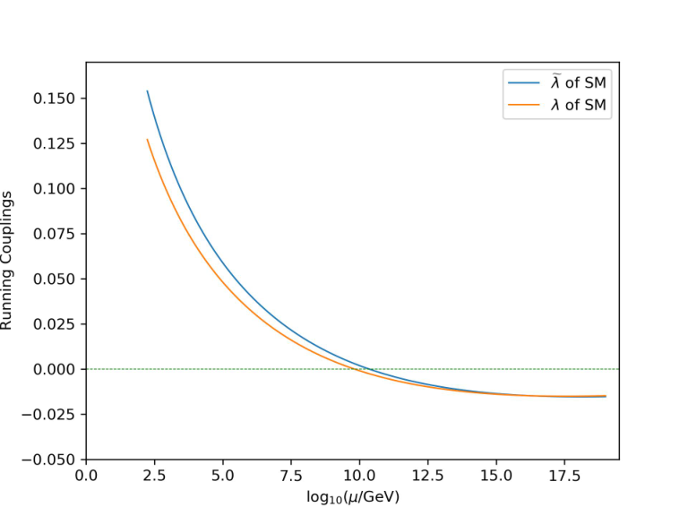
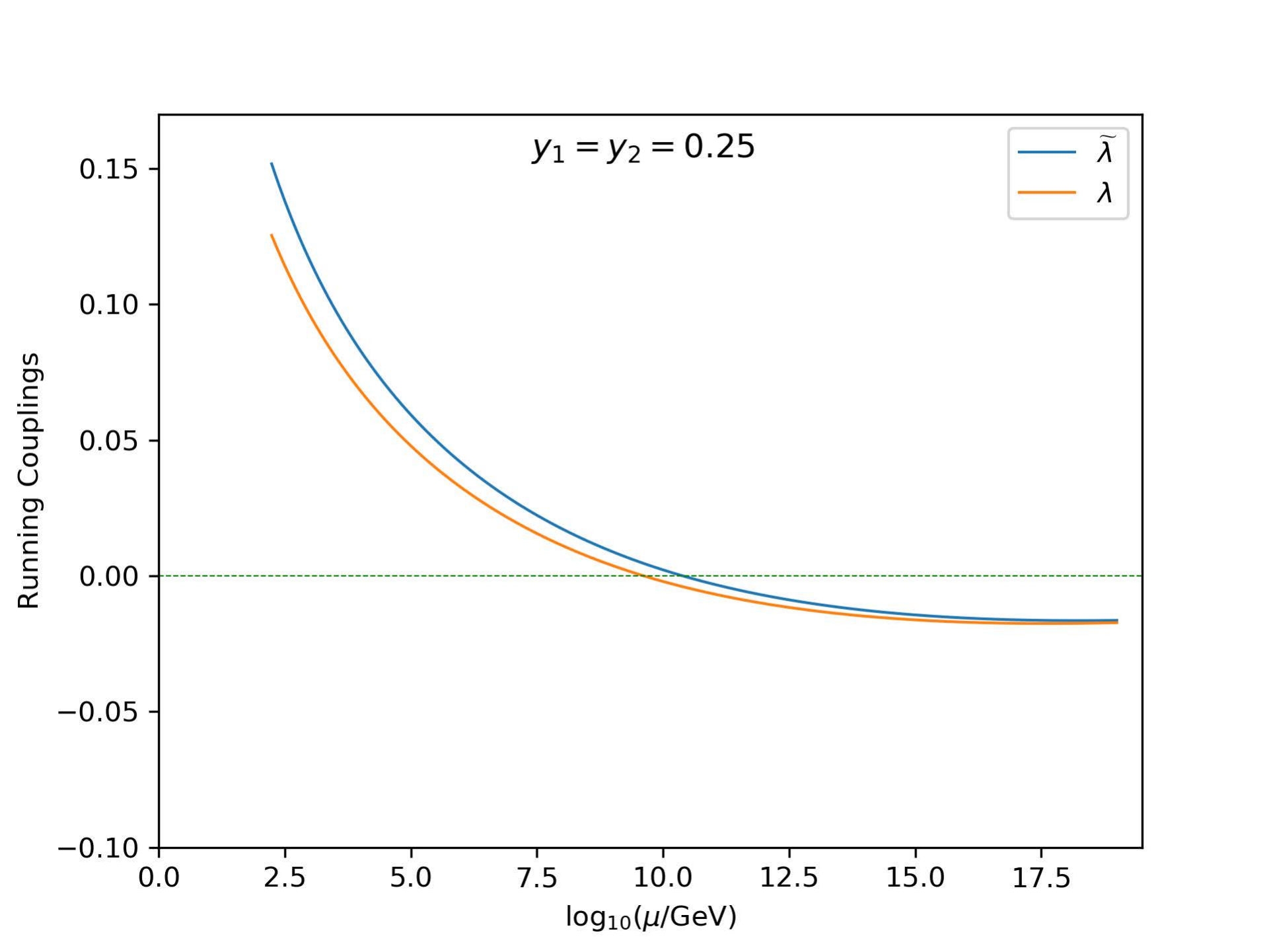
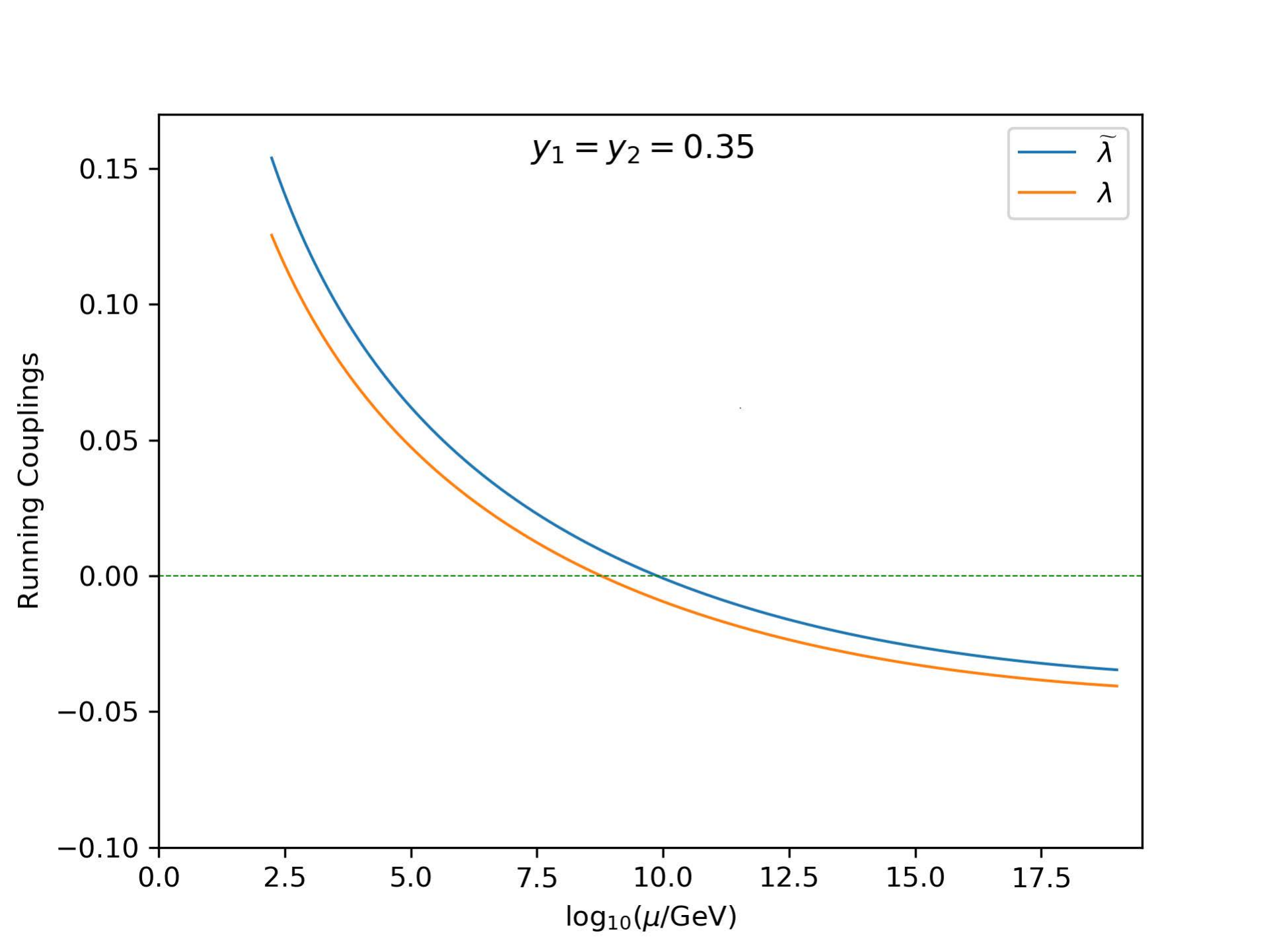
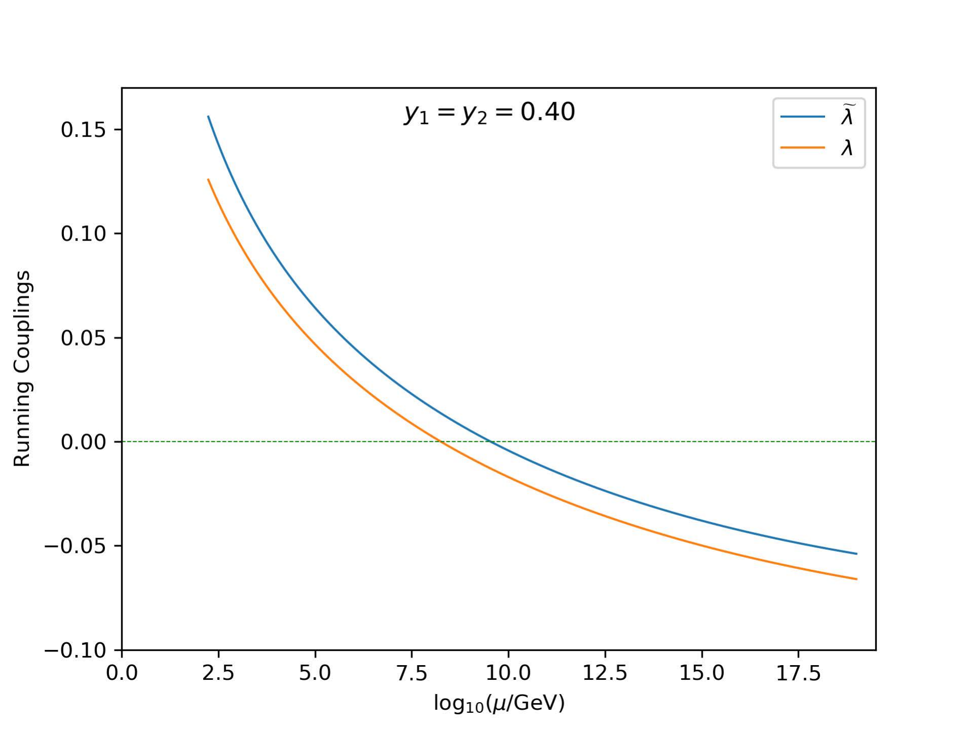
Now we come to discuss the tunneling probability. As shown in Eqs. (26), (35) and (37), the decay rate of false vacuum depends on Z2Z_{2} and λ~​(t){\tilde{\lambda}}(t) when including one-loop correction to the effective action. As mentioned before, the decay rate is mainly controlled by the behavior of λ~​(t){\tilde{\lambda}}(t). We first compare λ~​(t)\widetilde{\lambda}(t) and λ⁡(t)\lambda(t) in the SM. In the SM, λ~​(t)\widetilde{\lambda}(t) and λ⁡(t)\lambda(t) are very close at high energy scale, as shown in Fig. 3(a). They both approach the minimum before the Planck scale. Both the values of their minima and the energy scales of the minima are very close, as can be seen in Table 4. This means that the one loop corrections to effective potential have little effects on the tunneling probability in the SM. In the SDFDM model, the situation can be different. As can be seen in Fig. 3(b), λ~​(t)\widetilde{\lambda}(t) and λ⁡(t)\lambda(t) at high energy scale are not as close as in the SM. In this plot, λ~​(t)\widetilde{\lambda}(t) and λ⁡(t)\lambda(t) all approach their minima before the Planck scale. But their values at the minima and the energy scales of the minima are not as close as in the SM, as can be seen in Table 4. In Fig 4, we give more plots with larger y1y_{1} and y2y_{2}. In these cases, the difference between λ~​(t)\widetilde{\lambda}(t) and λ⁡(t)\lambda(t) is more significant. The larger the Yukawa coupling y1y_{1} and y2y_{2}, the larger the difference. We can see that the difference between λ~{\widetilde{\lambda}} and λ\lambda in Fig. 4(b) is not as significant as the difference between λe​f​f\lambda_{eff} and λ\lambda in Fig. 1(b). However, λ~−λ{\widetilde{\lambda}}-\lambda is still significant in this case. In these cases in Fig. 4, both λ~​(t)\widetilde{\lambda}(t) and λ⁡(t)\lambda(t) have no minimum for energy scale below the Planck scale. The energy scale of bounce, ΛB\Lambda_{B}, is chosen as the Planck scale for these two cases. We note that the positive sign of λ~−λ\widetilde{\lambda}-\lambda shown in Fig 4 means that the lifetime calculated using λ~\widetilde{\lambda} in these plots is longer than that computed by using λ\lambda.

Refer to caption
(a)
Refer to caption
(b)
Figure 3: (a)Comparison between λ\lambda and λ~\widetilde{\lambda} in the SM; (b) Comparison between λ\lambda and λ~{\tilde{\lambda}} with y1=y2=0.25y_{1}=y_{2}=0.25 and MS=MD=1000M_{S}=M_{D}=1000 GeV in the SDFDM model.
Refer to caption
(a)
Refer to caption
(b)
Figure 4: Comparison between λ⁡(t)\lambda(t) and λ~​(t){\tilde{\lambda}}(t) in the SDFDM model. (a) y1=y2=0.35y_{1}=y_{2}=0.35 and MS=MD=1000M_{S}=M_{D}=1000 GeV; (b) y1=y2=0.4y_{1}=y_{2}=0.4 and MS=MD=1000M_{S}=M_{D}=1000 GeV.

In Table. 4, we list more numerical results for the SM and for some benchmark points in the SDFDM model. As a comparison, we also list the results just using λ⁡(t)\lambda(t). We can see that using λ~​(t){\tilde{\lambda}}(t) and Z2Z_{2} in the effective action leads to some differences in the probability of false vacuum decay. For the case of the SM, we can see that the lifetime of EW vacuum computed using effective action is slightly longer than that computed just using λ⁡(t)\lambda(t) although λ~​(t){\tilde{\lambda}}(t) and λ⁡(t)\lambda(t) are very close at high energy scale. This is caused mainly by the presence of Z2Z_{2} in the effective action. In the SM, (Z2)2(Z_{2})^{2} term in Eq. (35) is about 1.02 which makes Sc​lS_{cl} slightly larger and leads to a smaller decay rate. In SDFDM model, the difference between λ~\widetilde{\lambda} and λ\lambda is significant, and the Z2Z_{2} factor increases with the increase of the Yukawa couplings y1y_{1} and y2y_{2}. Therefore, both the Z2Z_{2} factor and the increasing value of λ~−λ\widetilde{\lambda}-\lambda makes the lifetime calculated using effective action longer than that computed just using λ\lambda.

Refer to caption
(a)
Refer to caption
(b)
Figure 5: Status of the EW vacuum in the y1−y2y_{1}-y_{2} plane with MS=MD=1000M_{S}=M_{D}=1000 GeV . The left panel is given by using the ϕ4\phi^{4} potential and the running λ⁡(t)\lambda(t), and the right panel is computed by using effective action and λ~​(t){\tilde{\lambda}}(t). The green, blue, red regions indicate that the EW vacuum is metastable, unstable and non-perturbative.

In Fig. 5, we compare the two ways of obtaining the tunneling probability. The green(blue) region indicates that the EW vacuum is metastable(unstable), and the red region means that the EW vacuum is non-perturbative. We find that the one-loop effect on effective action slightly enlarges the parameter space for the vacuum to be metastable.

The parameter space of the singlet-doublet fermion dark matter model is constrained by phenomenological considerations of dark matter, such as the direct detection and the constraint from the dark matter relic density. It is found in Yaguna:2015mva that the dark matter Yukawa couplings must be very small, i.e. |y1|,|y2|≲4×10⁻³|y_{1}|,|y_{2}|\lesssim 4\times 10^{-3}, and that the masses of dark matter particle are constrained to be Mχ1≲733M_{\chi_{1}}\lesssim 733 GeV and |Mχ2−Mχ1|/Mχ1≲0.1|M_{\chi_{2}}-M_{\chi_{1}}|/M_{\chi_{1}}\lesssim 0.1. The vacuum stability analysis of this model does not give a constraint on the parameter space stronger than these phenomenological constraints.

IV General singlet-doublet fermion extension model

More general singlet-doublet fermion extension of the SM can be considered. In general, we can add N copies of SU⁡(2)\mathrm{SU}(2) doublet fermions ψL​n,R​n\psi_{Ln,Rn}(n=1,⋯,Nn=1,\cdots,N) and Q copies of singlet fermions SL​q,R​qS_{Lq,Rq}(q=1,⋯,Qq=1,\cdots,Q). The relevant Lagrangian can be written as

ℒgeneral\displaystyle\mathcal{L}_{\mathrm{general}} =∑n=1Nψ¯n​i/D​ψn+∑q=1QS¯q​i/∂Sq−∑n=1Nψ¯L​n​(M~D)n​n​ψR​n−∑q=1QS¯L​q​(M~S)q​q​SR​q\displaystyle=\sum_{n=1}^{N}\overline{\psi}_{n}i/\penalty\hskip-7.11317ptD\psi_{n}+\sum_{q=1}^{Q}\overline{S}_{q}i/\penalty\hskip-5.69046pt\partial S_{q}-\sum_{n=1}^{N}\overline{\psi}_{Ln}({\widetilde{M}}_{D})_{nn}\psi_{Rn}-\sum_{q=1}^{Q}\overline{S}_{Lq}({\widetilde{M}}_{S})_{qq}S_{Rq} (39)
−∑n=1N∑q=1Q(YR​n​qψ¯L​nH~SR​q+YL​n​qψ¯R​nH~SL​q)+h.c,\displaystyle-\sum_{n=1}^{N}\sum_{q=1}^{Q}\left(Y_{Rnq}\overline{\psi}_{Ln}\tilde{H}S_{Rq}+Y_{Lnq}\overline{\psi}_{Rn}\tilde{H}S_{Lq}\right)+h.c,

where we have chosen to work in the base that the mass matrices M~D{\widetilde{M}}_{D} and M~S{\widetilde{M}}_{S} are diagonal and real.

After the EW symmetry breaking, the mass matrix of the charged components of ψL​n,R​n\psi_{Ln,Rn}(ψL​n,R​n−\psi_{Ln,Rn}^{-}) are not changed. We simply denote ψL​n,R​n−\psi_{Ln,Rn}^{-} as χL​n,R​n−\chi^{-}_{Ln,Rn}. The N copies of neutral component of ψL​n,R​n\psi_{Ln,Rn}(ψL​n,R​n0\psi_{Ln,Rn}^{0}) and Q copies of SL​q,R​qS_{Lq,Rq} get a mass term. Introducing SL,R=(SL​1,R​1,⋯,SL​Q,R​Q)TS_{L,R}=(S_{L1,R1},\cdots,S_{LQ,RQ})^{T} and ψL,R=(ψL​1,R​1,⋯,ψL​N,R​N)T\psi_{L,R}=(\psi_{L1,R1},\cdots,\psi_{LN,RN})^{T}, we can write the mass term as

(S¯Lψ¯0L)​M​(SRψR0)+h.c.\begin{pmatrix}{\bar{S}}_{L}&{\bar{\psi}^{0}}_{L}\end{pmatrix}M\begin{pmatrix}S_{R}\\ \psi^{0}_{R}\end{pmatrix}+h.c. (40)

with the mass matrix MM given as

M=(M~Sv2​YL+v2​YRM~D.)M=\begin{pmatrix}{\widetilde{M}}_{S}&\frac{v}{\sqrt{2}}Y^{+}_{L}\\ \frac{v}{\sqrt{2}}Y_{R}&{\widetilde{M}}_{D}.\\ \end{pmatrix} (41)

Here YLY_{L} and YRY_{R} are the N×QN\times Q matrices of Yukawa coupling given in (39).

Performing a field transformation

(SL,RψL,R0)=UL,R​χL,R0\begin{pmatrix}S_{L,R}\\ \psi^{0}_{L,R}\end{pmatrix}=U_{L,R}\chi^{0}_{L,R} (42)

using two unitary matrices ULU_{L} and URU_{R} with χ0=(χ10,χ20,⋯,χN+Q0)T\chi^{0}=(\chi^{0}_{1},\chi^{0}_{2},\cdots,\chi^{0}_{N+Q})^{T} , the mass matrix MM can be diagonalized and becomes

Md=d​i​a​g​{Mχ10,Mχ20,⋯,MχN+Q0}=UL†​M​URM^{d}=diag\left\{{M_{\chi^{0}_{1}},M_{\chi^{0}_{2}},\cdots,M_{\chi^{0}_{N+Q}}}\right\}=U_{L}^{\dagger}MU_{R} (43)

where Mχi0M_{\chi^{0}_{i}} is the mass of χi0\chi^{0}_{i} field. The interaction Lagrangian of χi0\chi^{0}_{i} and the CP-even neutral Higgs field hh is obtained as

Δ​ℒh=−χ0¯​Y​PR​χ0​h−χ0¯​Y†​PL​χ0​h\Delta{\cal L}_{h}=-\overline{\chi^{0}}YP_{R}\chi^{0}h-\overline{\chi^{0}}Y^{\dagger}P_{L}\chi^{0}h (44)

where YY is the matrix of Yukawa coupling

Y=12​UL+​(0YL+YR0)​UR.Y=\frac{1}{\sqrt{2}}U^{+}_{L}\begin{pmatrix}0&Y^{+}_{L}\\ Y_{R}&0\\ \end{pmatrix}U_{R}. (45)

The interactions Lagrangian of χi0\chi^{0}_{i}, χn−\chi^{-}_{n} and the gauge bosons become

Δ​ℒW,Z=\displaystyle\Delta{\cal L}_{W,Z}= ∑n=1N[g22(UL+)i,n+Qχi0¯γμPLχn−W+μ+g22(UL)n+Q,iχn−¯γμPLχi0W−μ\displaystyle\sum_{n=1}^{N}\left[\frac{g_{2}}{{\sqrt{2}}}\left(U_{L}^{+}\right)_{i,n+Q}\overline{\chi_{i}^{0}}\gamma^{\mu}P_{L}\chi_{n}^{-}W^{+}_{\mu}+\frac{g_{2}}{{\sqrt{2}}}\left(U_{L}\right)_{n+Q,i}\overline{\chi_{n}^{-}}\gamma^{\mu}P_{L}\chi_{i}^{0}W^{-}_{\mu}\right. (46)
+g22​c​o​s​θw(UL+)i,n+Q(UL)n+Q,jχi0¯γμPLχj0Zμ+(L⟶R)]\displaystyle\left.+\frac{g_{2}}{2cos\theta_{w}}\left(U_{L}^{+}\right)_{i,n+Q}\left(U_{L}\right)_{n+Q,j}\overline{\chi_{i}^{0}}\gamma^{\mu}P_{L}\chi_{j}^{0}Z_{\mu}+(L\longrightarrow R)\right]
+∑n=1Nχn−¯(−g2sinθw/Aμ−g2​c​o​s​2​θw2​c​o​s​θw/Zμ)χn−.\displaystyle+\sum_{n=1}^{N}\overline{\chi_{n}^{-}}\left(-g_{2}sin\theta_{w}~/\penalty\hskip-7.11317ptA_{\mu}-\frac{g_{2}cos2\theta_{w}}{2cos\theta_{w}}\ /\penalty\hskip-7.11317ptZ_{\mu}\right)\chi_{n}^{-}.

Here θw\theta_{w} is the Weinberg angle.

In numerical analysis we consider three typical models.

IV.1 Model I

This model includes N copies of SU⁡(2)\mathrm{SU}(2) doublet fermions and N copies of singlet fermions. We assume the mass matrix matrices M~S{\widetilde{M}}_{S} and M~D{\widetilde{M}}_{D} are proportional to unit matrix. We also assume the Yukawa coupling YLY_{L} and YRY_{R} are diagonal and are proportional to the unit matrix. The relevant Lagrangian is

ℒModel​I\displaystyle\mathcal{L}_{\mathrm{Model\ I}} =∑n=1N(ψ¯n​i/D​ψn+S¯n​i/∂Sn−MD​ψ¯n​ψn−MS​S¯n​Sn)\displaystyle=\sum_{n=1}^{N}\left(\overline{\psi}_{n}i/\penalty\hskip-7.11317ptD\psi_{n}+\overline{S}_{n}i/\penalty\hskip-5.69046pt\partial S_{n}-M_{D}\overline{\psi}_{n}\psi_{n}-M_{S}\overline{S}_{n}S_{n}\right) (47)
−∑n=1N(y1ψ¯L​nH~SR​n+y2ψ¯R​nH~SL​n)+h.c\displaystyle-\sum_{n=1}^{N}\left(y_{1}\overline{\psi}_{Ln}\tilde{H}S_{Rn}+y_{2}\overline{\psi}_{Rn}\tilde{H}S_{Ln}\right)+h.c

This model basically introduces N generations of singlet-doublet fermions and there are no couplings between generations. So the mass matrix can be diagonalized in the same way as in Eq. (2) for each generation and there are N copies of neutral fermions χ1\chi_{1} and χ2\chi_{2} in the diagonalized base with masses given in (5) and (6).

IV.2 Model II

In this model we add N copies of SU⁡(2)\mathrm{SU}(2) doublet fermions ψL,R=(ψL,R0,ψL,R−)T\psi_{L,R}=\left(\psi_{L,R}^{0},\psi_{L,R}^{-}\right)^{T} and only one copy of singlet fermion SL,RS_{L,R}. The doublet fermions are all coupled with the only singlet. We assume that M~D{\widetilde{M}}_{D} are proportional to the unit matrix and all generations of doublet fermions couple with the singlet fermion with the same strength.

ℒModel​II\displaystyle\mathcal{L}_{\mathrm{Model\ II}} =∑n=1N(ψ¯n​i/D​ψn+S¯​i/∂S−MD​ψ¯n​ψn−MS​S¯​S)\displaystyle=\sum_{n=1}^{N}\left(\overline{\psi}_{n}i/\penalty\hskip-7.11317ptD\psi_{n}+\overline{S}i/\penalty\hskip-5.69046pt\partial S-M_{D}\overline{\psi}_{n}\psi_{n}-M_{S}\overline{S}S\right) (48)
−∑n=1N(y1ψ¯L​nH~SR+y2ψ¯R​nH~SL)+h.c.\displaystyle-\sum_{n=1}^{N}\left(y_{1}\overline{\psi}_{Ln}\tilde{H}S_{R}+y_{2}\overline{\psi}_{Rn}\tilde{H}S_{L}\right)+h.c.

After EW symmetry breaking, the mass matrix MM is obtained as

M=(MSy2​v2⋯y2​v2y1​v2MD⋯0⋱y1​v20⋯MD)M=\begin{pmatrix}M_{S}&\frac{y_{2}v}{\sqrt{2}}&\cdots&\frac{y_{2}v}{\sqrt{2}}\\ \frac{y_{1}v}{\sqrt{2}}&M_{D}&\cdots&0\\ \vdots&\vdots&\ddots&\vdots\\ \frac{y_{1}v}{\sqrt{2}}&0&\cdots\ &M_{D}\\ \end{pmatrix} (49)

In a suitable base, the singlet SS can be considered coupled only to one of the linear combinations of ψn\psi_{n}, i.e. Ψ=1N​∑n=1Nψn\Psi=\frac{1}{\sqrt{N}}\sum_{n=1}^{N}\psi_{n}, with effective couplings N​y1\sqrt{N}y_{1} and N​y2\sqrt{N}y_{2} in the new base. Other orthogonal linear combinations of ψn\psi_{n} do not couple to the singlet fermion. So the mass matrix can be diagonalized to a form

Md=d​i​a​g​{Mχ10,Mχ20,MD,⋯,MD},M^{d}=diag\left\{M_{\chi_{1}^{0}},M_{\chi_{2}^{0}},M_{D},\cdots,M_{D}\right\}, (50)

where the Mχ10M_{\chi_{1}^{0}} and Mχ20M_{\chi_{2}^{0}} are the masses of the two neutral fields, χ10\chi^{0}_{1} and χ20\chi^{0}_{2}, which couple to the neutral Higgs field. We can obtain

Mχ102=12​(TN−TN2−4​DN2),\displaystyle M_{\chi_{1}^{0}}^{2}=\frac{1}{2}(T_{N}-\sqrt{T_{N}^{2}-4~D_{N}^{2}}), (51)
Mχ202=12​(TN+TN2−4​DN2),\displaystyle M_{\chi_{2}^{0}}^{2}=\frac{1}{2}(T_{N}+\sqrt{T_{N}^{2}-4~D_{N}^{2}}), (52)

where TN=MS2+N2​y12​v2+MD2+N2​y22​v2T_{N}=M_{S}^{2}+\frac{N}{2}y_{1}^{2}v^{2}+M_{D}^{2}+\frac{N}{2}y_{2}^{2}v^{2}, DN=N2​y1​y2​v2−MS​MDD_{N}=\frac{N}{2}y_{1}y_{2}v^{2}-M_{S}M_{D}.

IV.3 Model III

In the third model, we consider extending the SM by adding N copies of singlet fermions SL,RS_{L,R} with only one copy of SU⁡(2)\mathrm{SU}(2) doublet fermion. The singlet fermions are all coupled with the only doublet. We assume that M~S{\widetilde{M}}_{S} are proportional to the unit matrix and all generations of singlet fermions couple with the doublet fermion with the same strength.

The mass matrix is given as:

M=(MS⋯0y2​v2⋱y2​v20⋯MSy1​v2y1​v2⋯MD).M=\begin{pmatrix}M_{S}&\cdots&0&\frac{y_{2}v}{\sqrt{2}}\\ \vdots&\ddots&\vdots&\frac{y_{2}v}{\sqrt{2}}\\ 0&\cdots&M_{S}&\vdots\\ \frac{y_{1}v}{\sqrt{2}}&\frac{y_{1}v}{\sqrt{2}}&\cdots\ &M_{D}\\ \end{pmatrix}. (53)

Similar to the case in Model II, the doublet ψ\psi can be considered coupled only to one of the linear combinations of SqS_{q}, i.e. 1N​∑q=1NSq\frac{1}{\sqrt{N}}\sum_{q=1}^{N}S_{q}, with effective couplings N​y1\sqrt{N}y_{1} and N​y2\sqrt{N}y_{2} in a suitable base. Other orthogonal linear combinations of SnS_{n} do not couple to the doublet fermion. So the mass matrix can be diagonalized to a form

Md=d​i​a​g​{Mχ10,Mχ20,MS,⋯,MS}M^{d}=diag\left\{M_{\chi_{1}^{0}},M_{\chi_{2}^{0}},M_{S},\cdots,M_{S}\right\} (54)

The Mχ10M_{\chi_{1}^{0}} and Mχ20M_{\chi_{2}^{0}} are the masses of the two neutral fields, χ10\chi^{0}_{1} and χ20\chi^{0}_{2}, which couple to the neutral Higgs field. The expressions of Mχ10M_{\chi^{0}_{1}} and Mχ20M_{\chi^{0}_{2}} are the same as in (51) and (52).

IV.4 Vacuum Stability in general singlet-doublet fermion extension models

In this section, we study the vacuum stability in the three models just introduced using RG improved effective action. For Model I, we can write down immediately the contribution to the RG improved effective potential following Eq. (21). We get

V1Ext​(ϕ,t)=N​∑i(−1)i​ni64​π2​Mχi4​(ϕ,t)​[ln⁡Mχi2​(ϕ,t)μ2​(t)−3/2].V_{1}^{\mathrm{Ext}}(\phi,t)=N\sum_{i}\frac{(-1)^{i}n_{i}}{64\pi^{2}}M_{\chi_{i}}^{4}(\phi,t)\left[\ln\frac{M_{\chi_{i}}^{2}(\phi,t)}{\mu^{2}(t)}-3/2\right]. (55)

For Model II and Model III, the RG improved effective potential can be obtained by simply substituting the neutral fermions masses (51) and (52) into Eq. (21).

Threshold corrections to couplings in general singlet-doublet fermion extension model are given in Appendix. D. In Table. 5, Table.  6 and Table. 7, we show some numerical results of couplings in the MS¯\overline{\mathrm{MS}} scheme for the three models shown above. New contributions to Z2Z_{2} factor in three models are shown Appendix D. The one-loop β\beta functions in the three models are given in Appendix D.1, D.2, D.3.

Threshold Effects for different N in Model​I\mathrm{Model\ I}
μ=Mt\quad\quad\mu=M_{t}\quad\quad λ\quad\quad\lambda\quad\quad   yty_{t}\quad\quad   g2g_{2}\quad\quad gY\quad\quad g_{Y}\quad\quad
N=2N=2 0.12495 0.93361∗ 0.64367 0.35859
N=5N=5 0.12330 0.92868∗ 0.63750 0.35902
N=7N=7 0.12221 0.92539∗ 0.63338 0.35932
Table 5: Threshold corrections to couplings when y1=y2=0.25y_{1}=y_{2}=0.25 for Model​I\mathrm{Model\ I}, MD=MS=1000M_{D}=M_{S}=1000 GeV. The superscript ∗* indicates that the NNNLO QCD effects are included.
Threshold Effects for different N in Model​II\mathrm{Model\ II}
μ=Mt\quad\quad\mu=M_{t}\quad\quad λ\quad\quad\lambda\quad\quad   yty_{t}\quad\quad   g2g_{2}\quad\quad gY\quad\quad g_{Y}\quad\quad
N=2N=2 0.12545 0.93480∗ 0.64367 0.35686
N=5N=5 0.12644 0.93164∗ 0.63750 0.35340
N=7N=7 0.12835 0.92954∗ 0.63714 0.34576
Table 6: Threshold corrections to couplings when y1=y2=0.2y_{1}=y_{2}=0.2 for Model​II\mathrm{Model\ II}, MD=MS=1000M_{D}=M_{S}=1000 GeV. The superscript ∗* indicates that the NNNLO QCD effects are included.
Threshold Effects for different N in Model​III\mathrm{Model\ III}
μ=Mt\quad\quad\mu=M_{t}\quad\quad λ\quad\quad\lambda\quad\quad   yty_{t}\quad\quad   g2g_{2}\quad\quad gY\quad\quad g_{Y}\quad\quad
N=2N=2 0.12545 0.93479∗ 0.64573 0.35809
N=5N=5 0.12644 0.93164∗ 0.64573 0.35563
N=7N=7 0.12835 0.92954∗ 0.64573 0.35400
Table 7: Threshold corrections to couplings when y1=y2=0.2y_{1}=y_{2}=0.2 for Model​III\mathrm{Model\ III}, MD=MS=1000M_{D}=M_{S}=1000 GeV. The superscript ∗* indicates that the NNNLO QCD effects are included.
Refer to caption
(a)
Refer to caption
(b)
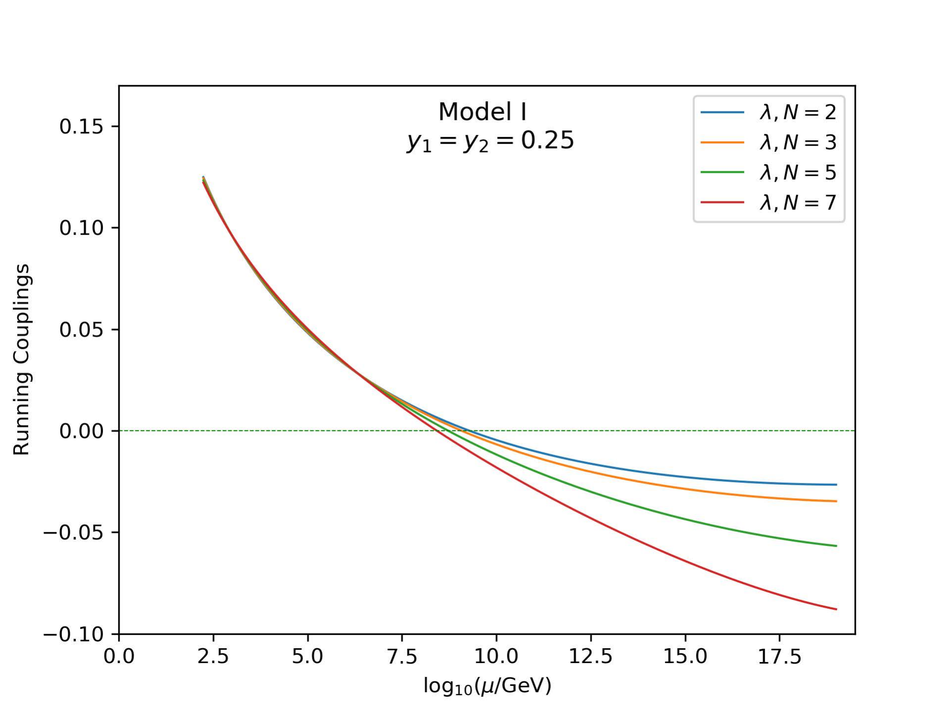
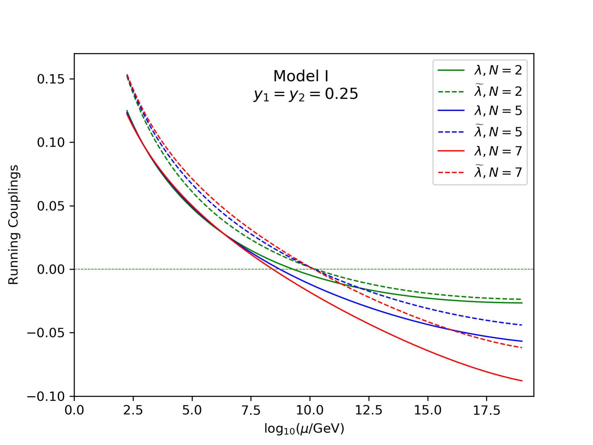
Figure 6: (a) λ⁡(t)\lambda(t) up to MP​lM_{Pl} for different values of N in Model I. The value of Yukawa couplings y1y_{1} and y2y_{2} are 0.250.25; (b) Running λ⁡(t)\lambda(t) and λ~​(t){\tilde{\lambda}}(t) up to MP​lM_{Pl} scale for N=2,5,7N=2,5,7 in Model I.
Refer to caption
(a)
Refer to caption
(b)
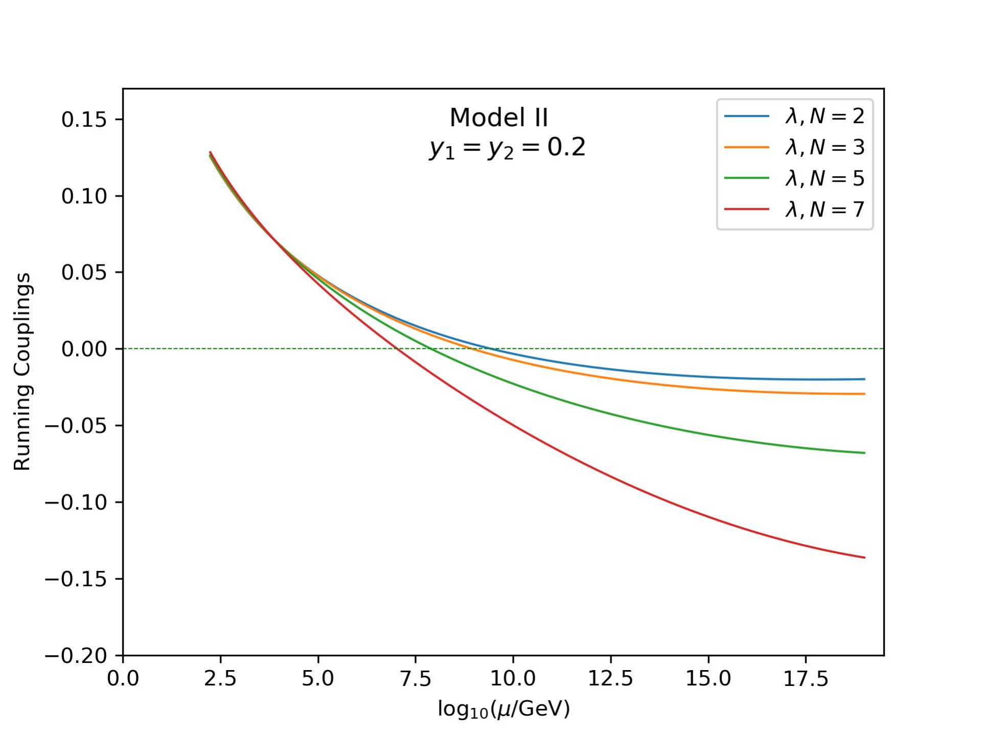
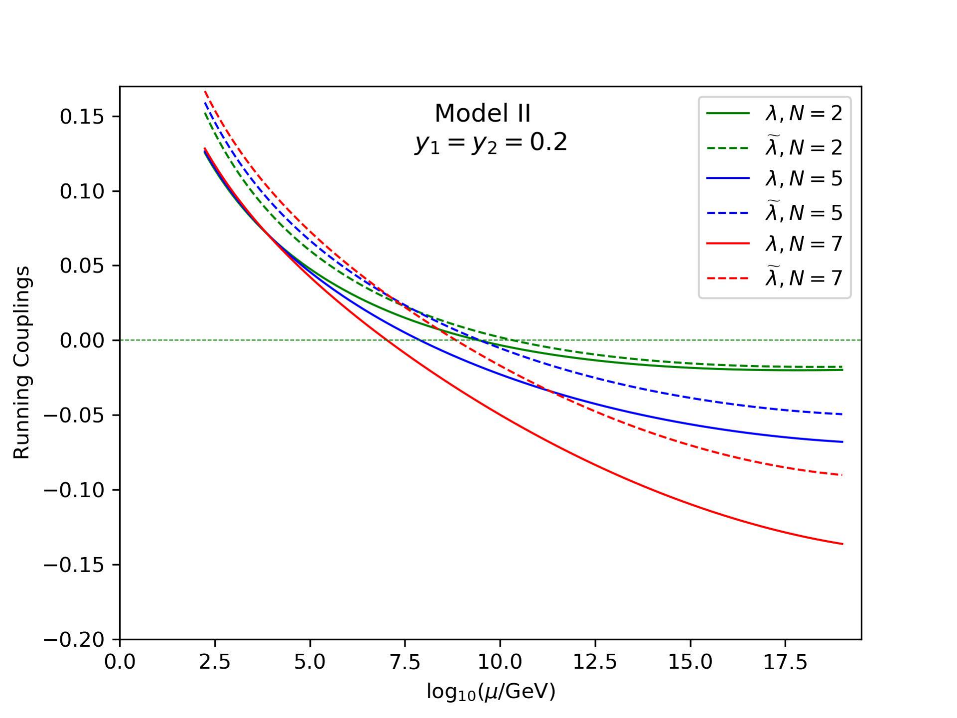
Figure 7: (a) λ⁡(t)\lambda(t) up to MP​lM_{Pl} for different values of N in Model II. The value of Yukawa couplings y1y_{1} and y2y_{2} are 0.20.2; (b) Running λ⁡(t)\lambda(t) and λ~​(t){\tilde{\lambda}}(t) up to MP​lM_{Pl} scale for N=2,5,7N=2,5,7 in Model II.
Refer to caption
(a)
Refer to caption
(b)
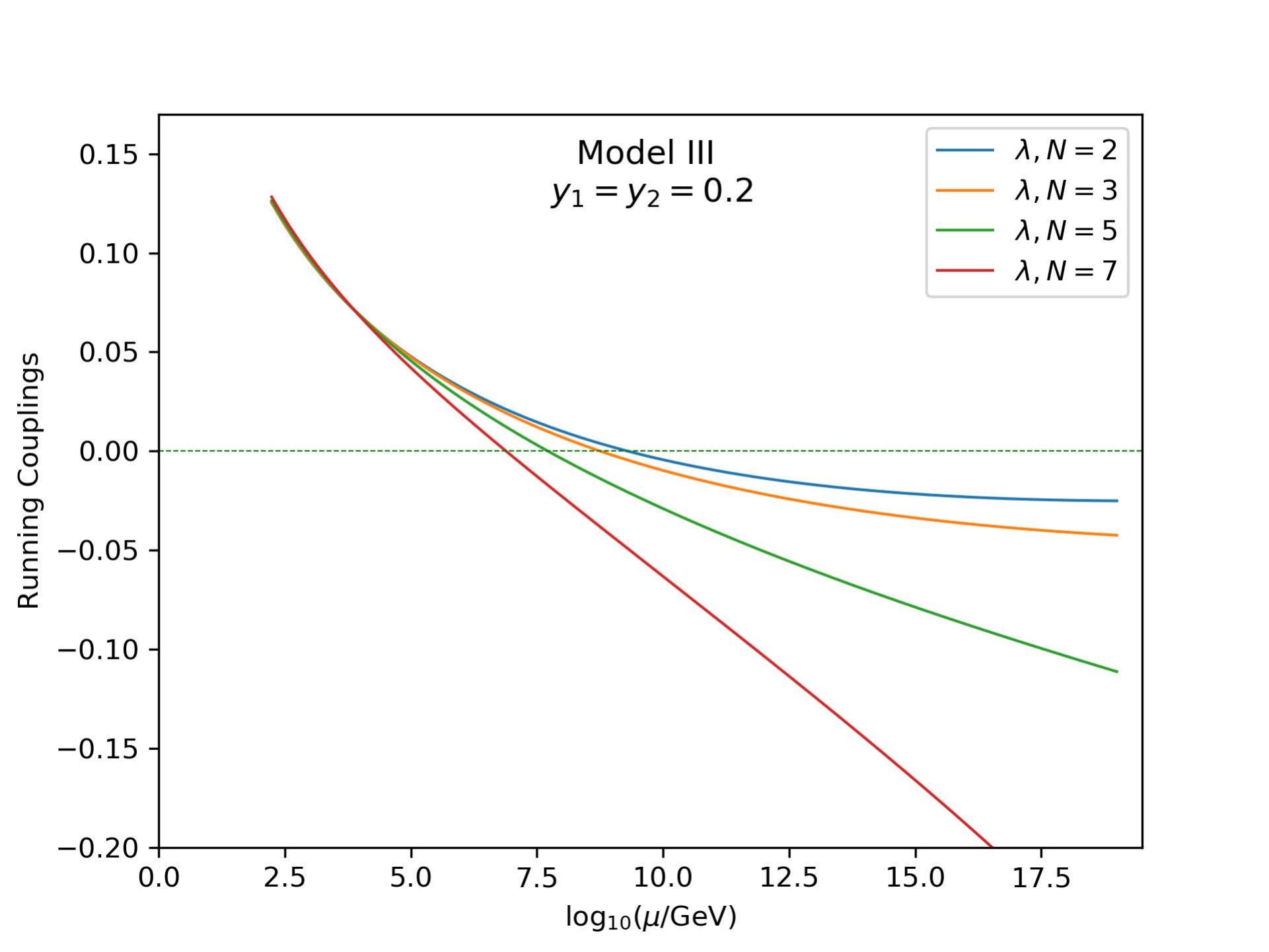
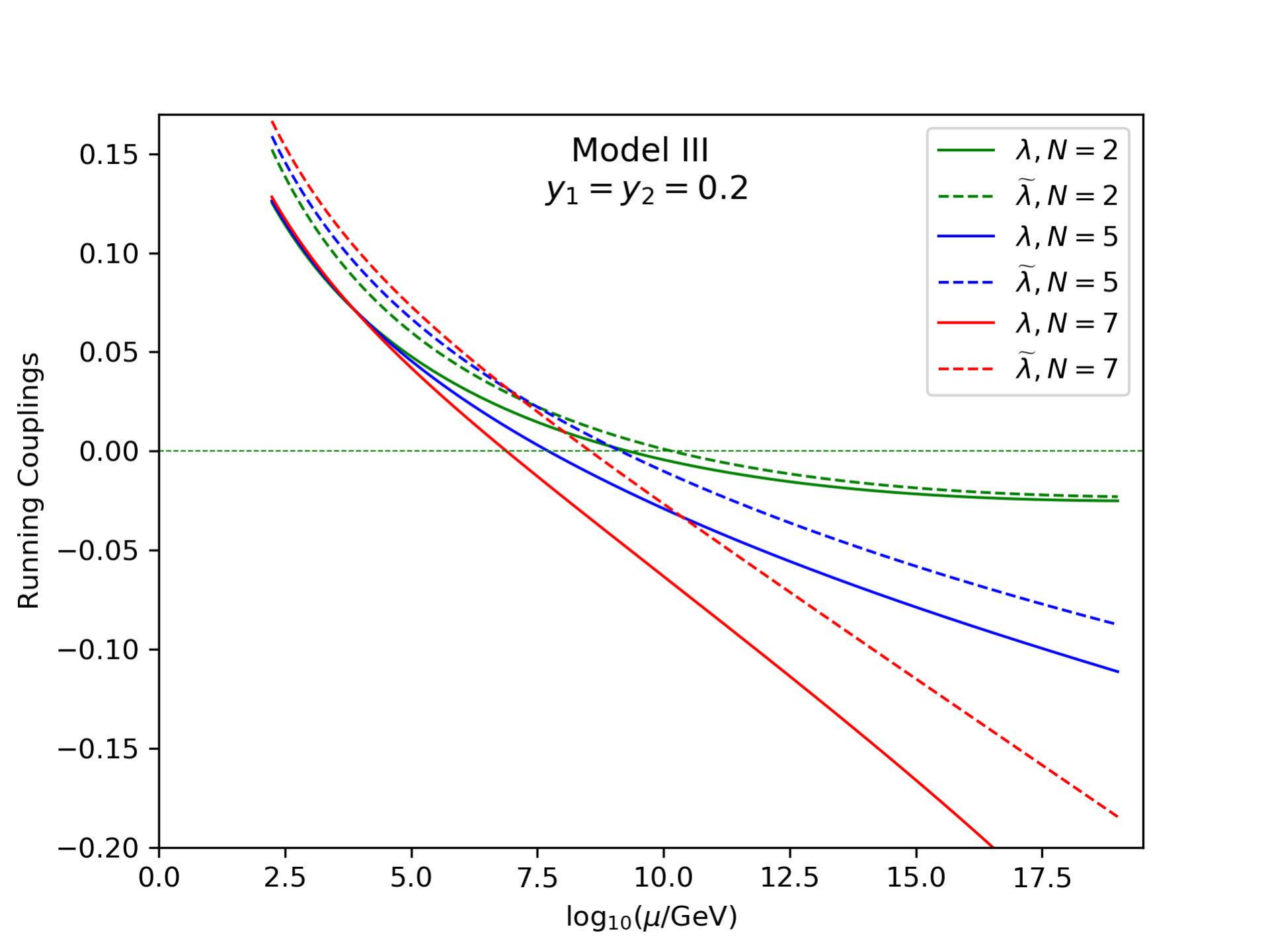
Figure 8: (a) λ⁡(t)\lambda(t) up to MP​lM_{Pl} for different values of N in Model III. The value of Yukawa couplings y1y_{1} and y2y_{2} are 0.20.2; (b) Running λ⁡(t)\lambda(t) and λ~​(t){\tilde{\lambda}}(t) up to MP​lM_{Pl} scale for N=2,5,7N=2,5,7 in Model III.
Refer to caption
(a)
Refer to caption
(b)
Figure 9: (a) Status of the EW vacuum in the y1−y2y_{1}-y_{2} plane for N=2,5,7N=2,5,7 in Model I; (b) Status of the EW vacuum in the y1−y2y_{1}-y_{2} plane for N=2,5,7N=2,5,7 in Model II. In both cases, the dashed line is the stable bound, the solid line the metastable bound, the dotted line the unstable bound.
Refer to caption
(a)
Refer to caption
(b)
Figure 10: (a)Status of the EW vacuum in the y1−y2y_{1}-y_{2} plane for N=2,5,7N=2,5,7 in Model III. The solid line is the metastable bound, the dotted line the unstable bound. (b) β\beta function of λ\lambda in Model I. The solid line is for y1=y2=0.1y_{1}=y_{2}=0.1, the dashed line for y1=y2=0.25y_{1}=y_{2}=0.25.
Refer to caption
(a)
Refer to caption
(b)
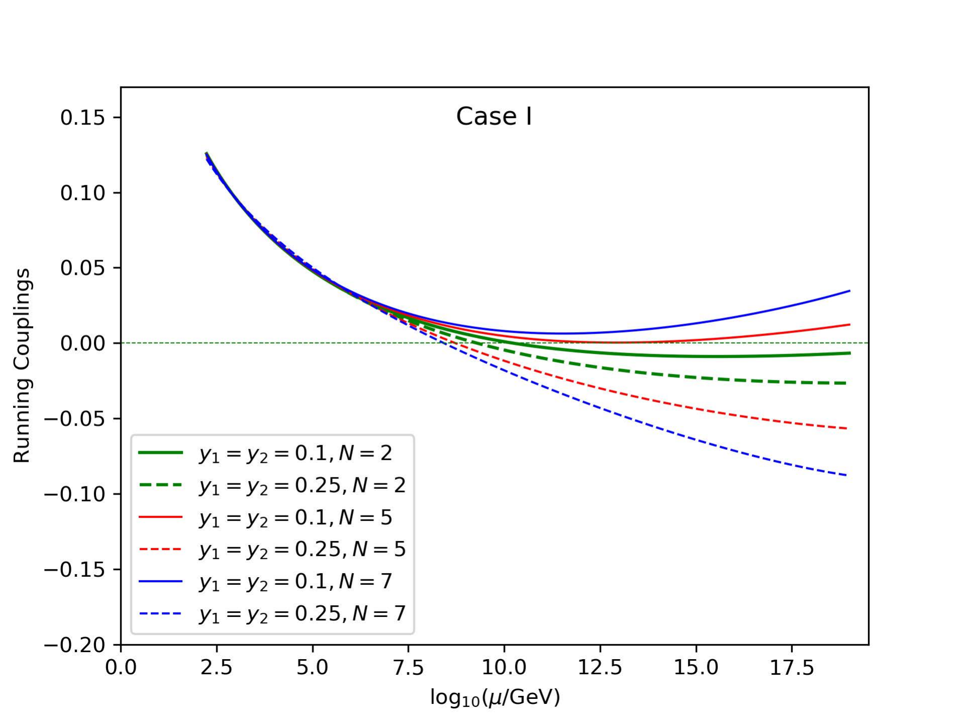
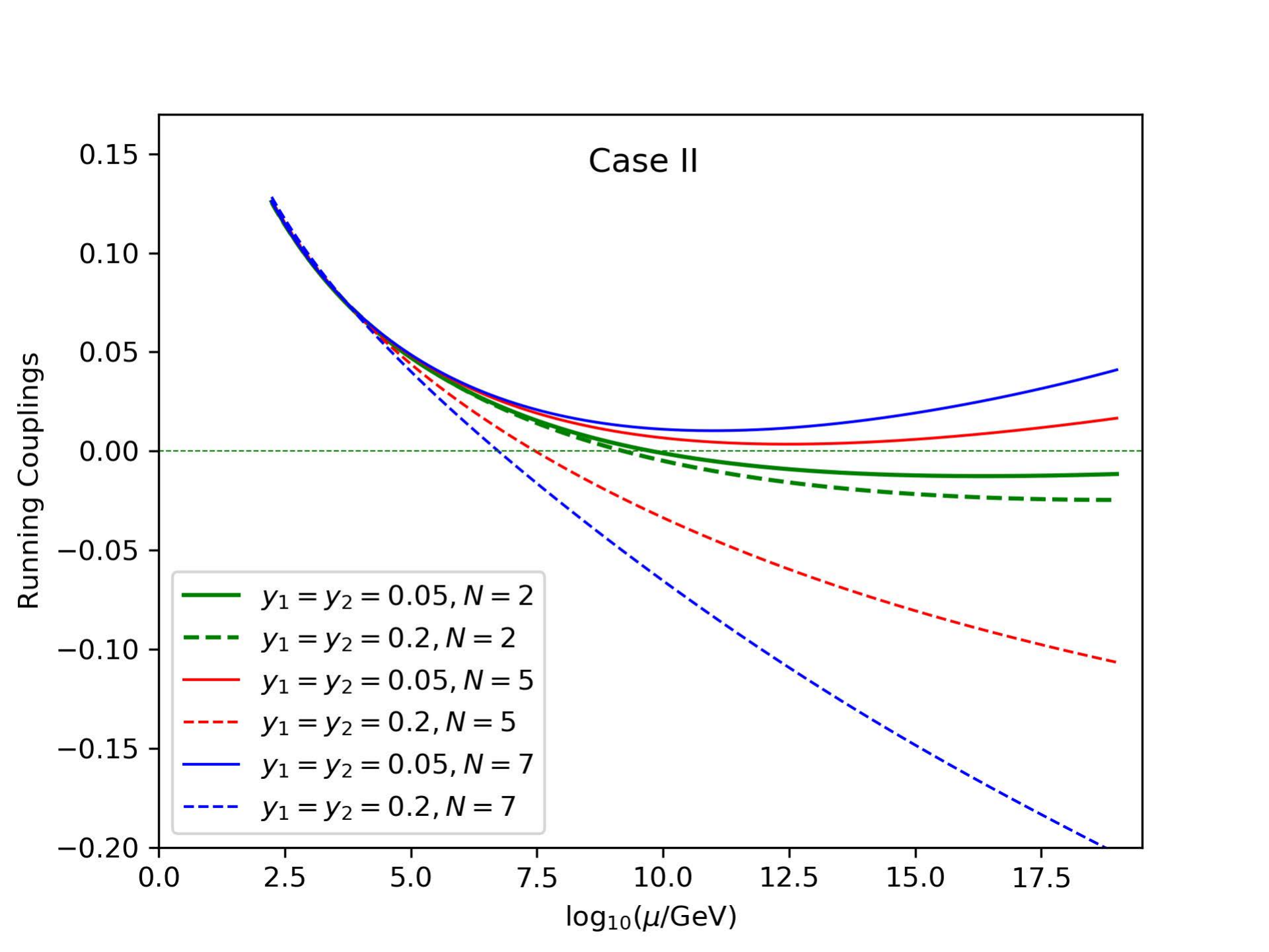
Figure 11: (a)λ⁡(t)\lambda(t) up to MP​lM_{Pl} for different values of Yukawa couplings in Model I, The solid lines are for y1=y2=0.1y_{1}=y_{2}=0.1 and the dashed lines for y1=y2=0.25y_{1}=y_{2}=0.25. (b) λ⁡(t)\lambda(t) up to MP​lM_{Pl} for different values of Yukawa couplings in Model II. The solid lines are for y1=y2=0.05y_{1}=y_{2}=0.05 and the dashed lines are for y1=y2=0.2y_{1}=y_{2}=0.2.

We can see the evolution of λ⁡(t)\lambda(t) in three models in Fig. 6(a), Fig. 7(a) and Fig. 8(a). Here we choose y1=y2=0.25y_{1}=y_{2}=0.25 in Model I and y1=y2=0.2y_{1}=y_{2}=0.2 in Model II and Model III. We can see that the minimum of λ⁡(t)\lambda(t) decreases as N is increased for these parameters in all these cases. In Fig. 6(b), 7(b) and Fig. 8(b),we compare the evolution of λ⁡(t)\lambda(t) and λ~\tilde{\lambda} in all models.The λ~\tilde{\lambda} is bigger than λ\lambda due to the one-loop Coleman-Weinberg type corrections. The difference between λ~\tilde{\lambda} and λ\lambda increases with the increase of N.

We study the status of EW vacuum in the y1−y2y_{1}-y_{2} plane for different N in the three models. Note that in Fig. 9(a) and Fig. 9(b), there are two types of lines for for N=2N=2, i.e. the solid line for the metastable bound, the dotted line for the unstable bound. For N=5N=5 and 77, there are three types of lines, i.e. and for N=5,7N=5,7, the dashed line for the stable bound, the solid line in the middle for the metastable bound and the dotted line for the unstable bound. In Fig. 10(a), there are two types of lines for all cases of N=2,5N=2,5 and 77, i.e. the solid line for the metastable bound and the dotted line for the unstable bound.

We can see that in both Model I and Model II the vacuum becomes stable when y1y_{1} and y2y_{2} are small and N is large. This is quite different from the result when N is small. In comparison, we can also see that in Model III, there are no such regions in the parameter space for which the EW vacuum becomes stable when N is large. This happens because the extra copies of fermion doublets in Model I and Model II give positive contributions to the β\beta functions of g1g_{1} and g2g_{2}, as can be seen in (123), (124), (132) and (133). For larger NN, this effect drives g1g_{1} and g2g_{2} running to larger values with faster rate. When y1y_{1} and y2y_{2} are small, the contribution of larger g1g_{1} and g2g_{2} can even make the β\beta function of λ\lambda turning into positive value, as can be seen in Fig. 10(b). If increasing the value of Yukawa coupling, the β\beta function can be turned into negative again, as can be seen in Fig. 10(b).

The impact of these running effects can be seen clearly in Fig. 11(a) and  11(b). In Fig. 11(a), we can see that λm​i​n>0\lambda_{min}>0 for y1=y2=0.1y_{1}=y_{2}=0.1 and N=5,7N=5,7. This means that the EW vacuum becomes stable for these parameters in Model I. On the contrary, λm​i​n<0\lambda_{min}<0 when y1=y2=0.25y_{1}=y_{2}=0.25 even for N=5N=5 and 77. We can also see in Fig. 11(b) that λm​i​n>0\lambda_{min}>0 when y1=y2=0.05y_{1}=y_{2}=0.05 and for both N=5N=5 and 77. This means that the EW vacuum becomes stable for these parameters in Model II. On the other hand, λm​i​n<0\lambda_{min}<0 when y1=y2=0.2y_{1}=y_{2}=0.2 in Model II. The results here are consistent with the results indicated in Fig. 9. When Yukawa couplings become bigger, λm​i​n<0\lambda_{min}<0 and the vacuum become unstable in both models.

We note that In Fig. 9(a), Fig. 9(b) and Fig. 10(a), we can also find that the metastable region and unstable region become smaller with the increase of N. This occurs because when y1y_{1} and y2y_{2} are bigger, the new physics effects of extra fermions would dominate the running of λ\lambda. More copies of extra fermions would make λ\lambda running faster to a negative value. We can similarly compare two ways of obtaining the tunneling probability, as done for SDFDM model in Fig. 5. The one-loop effective action again slightly modifies the parameter space presented in Fig. 9(a), Fig. 9(b) and Fig. 10(a).

V Conclusion

In summary, we have studied the one-loop Coleman-Weinberg type effective potential of the Higgs boson in a single-doublet fermion dark matter extension of the SM. We have calculated the threshold effect of these fermions in this model beyond the SM and have studied the RG running of parameters in the MS¯\overline{\mathrm{MS}} scheme. We have studied the RG improvement to the effective potential. We have studied the vacuum stability using the RG improved effective potential.

Using the method of derivative expansion, we have studied the quantum correction to the effective action. We have calculated the renormalization on the kinetic term in the effective action in the case with external field. We have studied the RG improvement of the kinetic term. Using the RG improved kinetic term and the RG improved effective potential, we calculate the decay rate of the false vacuum. We find that the factor arising from the anomalous dimension which appears in the kinetic term and the effective potential cancels in the decay rate. Taking all these considerations into account, we find that the decay rate of the false vacuum is slightly changed by the effective action.

We have also done all these studies in general singlet-doublet fermion extension models. We perform a numerical analysis in three typical extension models with N copies of single-doublet fermions, N copies of doublet fermions and N copies of singlet fermions separately. We find that several copies of fermion doublet can make the β\beta function of λ\lambda becoming positive in some regions of parameter space when Yukawa couplings of these extra fermions are small. Consequently, in models with small value of Yukawa couplings and large number of copies of fermion doublet, the EW vacuum can become stable. For large value of the Yukawa coupling, the EW vacuum can again be turned into metastable or unstable. We also find that the difference between Higgs self-coupling λ\lambda and λ~{\tilde{\lambda}}, the effective self-coupling after including Coleman-Weinberg type correction, becomes larger when the number of copies of singlet fermions or doublet fermions is increased. In the general singlet-doublet fermion extension models, the decay rate of the false vacuum is also slightly changed by the effective action.

Acknowledgements.
This work is supported by National Science Foundation of China(NSFC), grant No. 11875130.

Appendix A Threshold effect and parameters in the MS¯\overline{\mathrm{MS}} scheme

A.1 General strategy for one-loop matching

To study the vacuum stability of a model at high energy scale, we need to know the value of coupling constants at low energy scale and then run them to the Plank scale according to RGEs.To determine these parameters at low energy scale, the threshold corrections must be taken into account. In this article we use the strategy in Sirlin:1985ux; Buttazzo:2013uya to evaluate one-loop corrections. All the loop calculations are performed in the MS¯\overline{\mathrm{MS}} scheme in which all the parameters are gauge invariant and have gauge-invariant renormalisation group equations Caswell:1974cj.

A parameter in the MS¯\overline{\mathrm{MS}} scheme, e.g. θ⁡(μ¯)\theta(\overline{\mathrm{\mu}}), can be obtained from renormalized parameter θ\theta in physical scheme which is directly related to physical observables. The connection between θ\theta and θ⁡(μ¯)\theta(\overline{\mathrm{\mu}}) to one-loop order, can be found by noting that the unrenormalized θ0\theta_{0} is related to the renormalized couplings by

θ0=θ−δ​θ=θ⁡(μ¯)−δ​θMS\theta_{0}=\theta-\delta\theta=\theta(\overline{\mu})-\delta\theta_{\mathrm{MS}} (56)

where δ​θ\delta\theta and δ​θMS¯\delta\theta_{\overline{\mathrm{MS}}} are the corresponding counterterms. By definition δ​θMS¯\delta\theta_{\overline{\mathrm{MS}}} subtracts only the divergent part proportional to 1/ϵ+γ−ln⁡(4​π)1/{\epsilon}+\gamma-\mathrm{ln}(4\pi) in dimensional regularization with d=4−2​ϵd=4-2\epsilon being the space-time dimension. Since the divergent parts in the δ​θ\delta\theta and δ​θMS¯\delta\theta_{\overline{\mathrm{MS}}} counterterms are of the same form, θ⁡(μ¯)\theta(\overline{\mu}) can be rewritten as

θ⁡(μ¯)=θ−δ​θ|fin\theta(\overline{\mu})=\theta-\delta\theta|_{\mathrm{fin}} (57)

where the subscript fin denotes the finite part of the quantity δ​θ\delta\theta, obtained after subtracting the terms proportional to 1/ϵ+γ−ln⁡(4​π)1/{\epsilon}+\gamma-\mathrm{ln}(4\pi). Difference at two-loop order has been neglected in this expression.

The physical parameters which would be used in Eq. (57), such as μ2\mu^{2} and λ\lambda, the quadratic and quartic couplings in the Higgs potential, the vacuum expectation value vv, the top Yukawa coupling yty_{t}, the gauge couplings g2g_{2} and gYg_{Y} of SU​(2)L×U​(1)Y\mathrm{SU}(2)_{\mathrm{L}}\times\mathrm{U}(1)_{\mathrm{Y}} group, can be determined from physical observables, such as the pole mass of the Higgs boson (Mh)\left(M_{h}\right), the pole mass of the top quark (Mt)\left(M_{t}\right), the pole mass of the Z boson (MZ)\left(M_{Z}\right), the pole mass of the W boson (MW)\left(M_{W}\right), and the Fermi constant (Gμ)\left(G_{\mu}\right). These physical observables are listed in Table. 8. If knowing the corresponding counterterms in the physical scheme, the MS¯\overline{\mathrm{MS}} couplings are then obtained using (57). For example, if knowing δ​λ\delta\lambda, we then obtain λ⁡(μ¯)\lambda(\overline{\mu}) in the MS¯\overline{\mathrm{MS}} scheme. More details are explained as follows.

Input values of SM observables
  Observables  Values
MWM_{W} 80.384±0.01480.384\pm 0.014 GeV
MZM_{Z} 91.1876±0.002191.1876\pm 0.0021 GeV
MhM_{h} 125.15±0.24125.15\pm 0.24 GeV
MtM_{t} 173.34±0.76173.34\pm 0.76 GeV
v=(2Gμ)−1/2v=(\sqrt{2}G_{\mu})^{-1/2}  246.21971±0.00006246.21971\pm 0.00006 GeV
α3​(MZ)\alpha_{3}({M}_{Z}) 0.1184±0.00070.1184\pm 0.0007
Table 8: Input values of physical observables used to fix the SM fundamental parameters λ\lambda, mm, yty_{t}, g2g_{2}, and gYg_{Y}. MWM_{W}, MZM_{Z}, MhM_{h}, and MtM_{t} are the pole masses of the WW boson, of the ZZ boson, of the Higgs boson, and of the top quark, respectively. GμG_{\mu} is the Fermi constant for μ\mu decay, and α3\alpha_{3} is the S​U​(3)cSU(3)_{c} gauge coupling at the scale μ=MZ\mu=M_{Z} in the MS¯\overline{\mathrm{MS}} scheme.

We follow Ref. Sirlin:1985ux to fix the notation. We write the classical Higgs potential in bare quantities as

V=−μ02​Φ†​Φ+λ0​(Φ†​Φ)2V=-\mu_{0}^{2}\Phi^{\dagger}\Phi+\lambda_{0}\left(\Phi^{\dagger}\Phi\right)^{2} (58)

with

Φ=(ϕ+12​(ϕ1+i​ϕ2+v0))\Phi=\left(\begin{array}[]{c}{\phi^{+}}\\ {\sqrt{\frac{1}{2}}\left(\phi_{1}+i\phi_{2}+v_{0}\right)}\end{array}\right) (59)

Setting λ0=λ−δ​λ,v0=v−δ​v,μ02=μ2−δ​μ2\lambda_{0}=\lambda-\delta\lambda,v_{0}=v-\delta v,\mu_{0}^{2}=\mu^{2}-\delta\mu^{2}, where λ\lambda, vv and μ\mu are regarded as renormalized quantities, we write

V=V(r)−δ​VV=V_{(r)}-\delta V (60)

with

V(r)=\displaystyle V_{(\mathrm{r})}= λ⁡[ϕ+​ϕ−​(ϕ+​ϕ−+ϕ12+ϕ22)+14​(ϕ12+ϕ22)2]\displaystyle\lambda\left[\phi^{+}\phi^{-}\left(\phi^{+}\phi^{-}+\phi_{1}^{2}+\phi_{2}^{2}\right)+\frac{1}{4}\left(\phi_{1}^{2}+\phi_{2}^{2}\right)^{2}\right] (61)
+λ​v​ϕ1​[ϕ12+ϕ22+2​ϕ+​ϕ−]+2​λ​v2​12​ϕ12\displaystyle+\lambda v\phi_{1}\left[\phi_{1}^{2}+\phi_{2}^{2}+2\phi^{+}\phi^{-}\right]+2\lambda v^{2}\frac{1}{2}\phi_{1}^{2}

and

δ​V=\displaystyle\delta V= δ​λ​[(ϕ+​ϕ−)​(ϕ+​ϕ−+ϕ12+ϕ22)+14​(ϕ12+ϕ22)2]\displaystyle\delta\lambda\left[\left(\phi^{+}\phi^{-}\right)\left(\phi^{+}\phi^{-}+\phi_{1}^{2}+\phi_{2}^{2}\right)+\frac{1}{4}\left(\phi_{1}^{2}+\phi_{2}^{2}\right)^{2}\right] (62)
+[λ​δ​v+v​δ​λ]​ϕ1​[ϕ12+ϕ22+2​ϕ+​ϕ−]+δ​τ​[ϕ+​ϕ−+12​ϕ22]\displaystyle+[\lambda\delta v+v\delta\lambda]\phi_{1}\left[\phi_{1}^{2}+\phi_{2}^{2}+2\phi^{+}\phi^{-}\right]+\delta\tau\left[\phi^{+}\phi^{-}+\frac{1}{2}\phi_{2}^{2}\right]
+δ​Mh2​12​ϕ12+v​δ​τ​ϕ1\displaystyle+\delta M_{\mathrm{h}}^{2}\frac{1}{2}\phi_{1}^{2}+v\delta\tau\phi_{1}

where

δ​Mh2\displaystyle\delta M_{\mathrm{h}}^{2} =3​v2​δ​λ+6​λ​v​δ​v−δ​μ2,\displaystyle=3v^{2}\delta\lambda+6\lambda v\delta v-\delta\mu^{2}, (63)
δ​τ\displaystyle\delta\tau =v2​δ​λ+2​λ​v​δ​v−δ​μ2.\displaystyle=v^{2}\delta\lambda+2\lambda v\delta v-\delta\mu^{2}. (64)

vv is determined at tree-level by GμG_{\mu} as shown in Table. 8.

In order to determine δ​λ\delta\lambda, δ​v\delta v and δ​μ2\delta\mu^{2} we need three constraints. The strategy is to adjust δ​τ\delta\tau so that the v​δ​τ​ϕ1v\delta\tau\phi_{1} term in Eq. 62 cancels the tadpole diagrams. Calling i​TiT the sum of the tadpole diagrams with the external legs extracted, we have the condition

δτ=−T/v.\delta\tau=-T/v. (65)

A second constraint is conveniently obtained by demanding that the coefficient of the term proportional to 12​ϕ12\frac{1}{2}\phi_{1}^{2} in V(r)V_{(\mathrm{r})} be the physical mass of the Higgs boson. So we have

Mh2=2​λ​v2M_{\mathrm{h}}^{2}=2\lambda v^{2} (66)

and δ​Mh2\delta M_{\mathrm{h}}^{2} is fixed by condition of on-shell renormalization, i.e.

δ​Mh2=Re⁡Πhh​(Mh2),\displaystyle\delta M_{\mathrm{h}}^{2}=\operatorname{Re}\Pi_{\mathrm{hh}}\left(M_{\mathrm{h}}^{2}\right), (67)

where Πhh​(Mh2)\Pi_{\mathrm{hh}}\left(M_{\mathrm{h}}^{2}\right) is the Higgs boson self-energy evaluated on shell. A third constraint is provided by Eq. (9b) of Ref. Sirlin:1980nh

δ​MW2=Re⁡Πw​w​(MW2),\delta M_{W}^{2}=\operatorname{Re}\Pi_{ww}\left(M_{W}^{2}\right), (68)

where Πw​w​(MW2)\Pi_{ww}\left(M_{W}^{2}\right) is the W boson self-energy evaluated on shell. Recalling that the W-mass counterterm is given by Sirlin:1980nh

δ​MW2=12​(v2​g2​δ​g2+g22​v​δ​v),\delta M_{\mathrm{W}}^{2}=\frac{1}{2}\left(v^{2}g_{2}\delta g_{2}+g_{2}^{2}v\delta v\right), (69)

δ​v\delta v is obtained using this expression with δ​g2\delta g_{2} known from other condition which can be found in Eq. (28a) of Sirlin:1980nh. Putting δ​v\delta v, Eqs. (67) and (69) into (63) and (64), one can then obtain δ​λ\delta\lambda and δ​μ2\delta\mu^{2}. They are as follows.

δ​μ2=\displaystyle\delta\mu^{2}= 12​[Re⁡Πhh​(Mh2)+3​T/v],\displaystyle\frac{1}{2}\left[\operatorname{Re}\Pi_{\mathrm{hh}}\left(M_{\mathrm{h}}^{2}\right)+3T/v\right], (70)
δ​λ/λ=\displaystyle\delta\lambda/\lambda= [Re⁡Πhh​(Mh2)+T/v]/Mh2−Re⁡Πww​(MW2)/MW2+2​δ​g2/g2,\displaystyle\left[\operatorname{Re}\Pi_{\mathrm{hh}}\left(M_{\mathrm{h}}^{2}\right)+T/v\right]/M_{\mathrm{h}}^{2}-\operatorname{Re}\Pi_{\mathrm{ww}}\left(M_{\mathrm{W}}^{2}\right)/M_{\mathrm{W}}^{2}+2\delta g_{2}/g_{2}, (71)
δ​v/v=\displaystyle\delta v/v= Re⁡Πww​(MW2)/(2​MW2)−δ​g2/g2\displaystyle\operatorname{Re}\Pi_{\mathrm{ww}}\left(M_{\mathrm{W}}^{2}\right)/\left(2M_{\mathrm{W}}^{2}\right)-\delta g_{2}/g_{2} (72)

We can get the expressions of the counterterms of the other parameters in a similar way.

Ignoring the contribution of higher order, we list the one-loop results of counterterms as follows.

δ(1)​λ\displaystyle\delta^{(1)}\lambda =Gμ2​Mh2​{Δ​r0(1)+1Mh2​[T(1)v+Re⁡Πh​h​(Mh2)]},\displaystyle=\frac{G_{\mu}}{\sqrt{2}}M_{h}^{2}\left\{\Delta r_{0}^{(1)}+\frac{1}{M_{h}^{2}}\left[\frac{T^{(1)}}{v}+\operatorname{Re}\Pi_{hh}\left(M_{h}^{2}\right)\right]\right\}, (73)
δ(1)​yt\displaystyle\delta^{(1)}y_{t} =2​(Gμ2​Mt2)1/2​(Re⁡Πt​t​(Mt2)Mt+Δ​r0(1)2),\displaystyle=2\left(\frac{G_{\mu}}{\sqrt{2}}M_{t}^{2}\right)^{1/2}\left(\frac{\operatorname{Re}\Pi_{tt}\left(M_{t}^{2}\right)}{M_{t}}+\frac{\Delta r_{0}^{(1)}}{2}\right), (74)
δ(1)​g2\displaystyle\delta^{(1)}g_{2} =(2​Gμ)1/2​MW​(Re⁡Πw​w​(MW2)MW2+Δ​r0(1)),\displaystyle=\left(\sqrt{2}G_{\mu}\right)^{1/2}M_{W}\left(\frac{\operatorname{Re}\Pi_{ww}\left(M_{W}^{2}\right)}{M_{W}^{2}}+\Delta r_{0}^{(1)}\right), (75)
δ(1)​gY\displaystyle\delta^{(1)}g_{Y} =(2​Gμ)1/2​MZ2−MW2​(Re⁡Πz​z​(MZ2)−Re⁡Πw​w​(MW2)MZ2−MW2+Δ​r0(1)),\displaystyle=\left(\sqrt{2}G_{\mu}\right)^{1/2}\sqrt{M_{Z}^{2}-M_{W}^{2}}\left(\frac{\operatorname{Re}\Pi_{zz}\left(M_{Z}^{2}\right)-\operatorname{Re}\Pi_{ww}\left(M_{W}^{2}\right)}{M_{Z}^{2}-M_{W}^{2}}+\Delta r_{0}^{(1)}\right), (76)

where superscripts 11 in these equations indicate that they are results at one-loop order. Δ​r0(1)\Delta r_{0}^{(1)} in the above equations can be written as a sum of several terms Buttazzo:2013uya

Δ​r0(1)=VW(1)−AW​W(1)MW2+2Gμ​ℬW(1)+ℰ(1)\Delta r_{0}^{(1)}=V_{W}^{(1)}-\frac{A_{WW}^{(1)}}{M_{W}^{2}}+\frac{\sqrt{2}}{G_{\mu}}\mathcal{B}_{W}^{(1)}+\mathcal{E}^{(1)} (77)

where AW​WA_{WW} is the WW boson self-energy at zero momentum, VWV_{W} the vertex contribution in the muon decay process, ℬW{\cal B}_{W} the box contribution, ℰ{\cal E} a term due to the renormalization of external legs. They are all computed at zero external momentum. Thus we eventually get the MS¯\overline{\mathrm{MS}} parameter to one-loop order as follows Buttazzo:2013uya; Wang:2018lhk.

λ⁡(μ¯)\displaystyle\lambda(\overline{\mathrm{\mu}}) =Gμ2​Mh2−δ(1)​λ|fin,\displaystyle=\frac{G_{\mu}}{\sqrt{2}}M_{h}^{2}-\delta^{(1)}\left.\lambda\right|_{\mathrm{fin}}, (78)
yt​(μ¯)\displaystyle y_{t}(\overline{\mathrm{\mu}}) =2​(Gμ2​Mt2)1/2−δ(1)​yt|fin,\displaystyle=2\left(\frac{G_{\mu}}{\sqrt{2}}M_{t}^{2}\right)^{1/2}-\delta^{(1)}\left.y_{t}\right|_{\mathrm{fin}}, (79)
g2​(μ¯)\displaystyle g_{2}(\overline{\mathrm{\mu}}) =2​(2​Gμ)1/2​MW−δ(1)​g2|fin,\displaystyle=2\left(\sqrt{2}G_{\mu}\right)^{1/2}M_{W}-\delta^{(1)}\left.g_{2}\right|_{\mathrm{fin}}, (80)
gY​(μ¯)\displaystyle g_{Y}(\overline{\mathrm{\mu}}) =2​(2​Gμ)1/2​MZ2−MW2−δ(1)​gY|fin.\displaystyle=2\left(\sqrt{2}G_{\mu}\right)^{1/2}\sqrt{M_{Z}^{2}-M_{W}^{2}}-\delta^{(1)}\left.g_{Y}\right|_{\mathrm{fin}}. (81)

A.2 MS¯\overline{\mathrm{MS}} parameters in the SDFDM model

To determine the initial values of running couplings, we use the equations given in the last section. Since the threshold corrections have been done to NNLO in the SM, we only need to calculate the contribution of extra fermions in the SDFDM model. All the relevant Feynman diagrams for computing δ(1)​λ|fin\delta^{(1)}\left.\lambda\right|_{\mathrm{fin}} with extra fermions are listed in Fig. 12.

Refer to caption
Refer to caption
Refer to caption
Refer to caption
Refer to caption
Figure 12: Contributions of extra fermions to the self-energy for (a) the Higgs boson, (b)ZZ boson, and (d)(e) WW bosons, as well as to (c) the tadpole of the Higgs boson. χ(1,2)\chi_{(1,2)} are dark sector fermions.

As singlet-doublet fermions in SDFDM model do not couple to SM leptons, Eq. (77) can be further simplified as

Δ​r0=−AW​WMW2.\Delta r_{0}=-\frac{A_{WW}}{M_{W}^{2}}. (82)

Summing over all the loop contributions and using the matching conditions, we get coupling constants in the MS¯{\overline{\mathrm{MS}}} scheme at Mt=173​GeVM_{t}=173~\mathrm{GeV} energy scale and for the SDFDM model respectively.

We summarize here the one-loop corrections to λ\lambda from new particles in SDFDM model by using Eq. (73). We write δ(1)​λS​D​F​D​M\delta^{(1)}\lambda_{SDFDM} in terms of finite parts of the Passarino-Veltman functions

A0(M)=M2(1−lnM2μ¯2),B0(M1,M2,p)=−∫01lnx​M12+(1−x)​M22−x⁡(1−x)​p2μ¯2dx.A_{0}(M)=M^{2}\left(1-\ln\frac{M^{2}}{\overline{\mu}^{2}}\right),~B_{0}\left(M_{1},M_{2},p\right)=-\int_{0}^{1}\ln\frac{xM_{1}^{2}+(1-x)M_{2}^{2}-x(1-x)p^{2}}{\overline{\mu}^{2}}dx. (83)

The one-loop result is

δ(1)​λ|f​i​n=\displaystyle\delta^{(1)}\lambda|_{fin}= Gμ2​(4​π)2{yA2[4A0(Mχ10)−2(M2h−4M2χ10)B0(Mχ10,Mχ10,Mh)]\displaystyle\frac{G_{\mu}}{\sqrt{2}(4\pi)^{2}}\left\{y_{A}^{2}[4A_{0}(M_{\chi_{1}^{0}})-2(M^{2}_{h}-4M^{2}_{\chi_{1}^{0}})B_{0}(M_{\chi_{1}^{0}},M_{\chi_{1}^{0}},M_{h})]\right. (84)
+yB2​[4​A0​(Mχ20)−2​(Mh2−4​Mχ202)​B0​(Mχ20,Mχ20,Mh)]\displaystyle+y_{B}^{2}[4A_{0}(M_{\chi_{2}^{0}})-2(M^{2}_{h}-4M^{2}_{\chi_{2}^{0}})B_{0}(M_{\chi_{2}^{0}},M_{\chi_{2}^{0}},M_{h})]
+2​yC2​[A0​(Mχ10)+A0​(Mχ20)−(Mh2−Mχ102−Mχ202)​B0​(Mχ10,Mχ20,Mh)]\displaystyle+2y_{C}^{2}[A_{0}(M_{\chi_{1}^{0}})+A_{0}(M_{\chi_{2}^{0}})-(M^{2}_{h}-M^{2}_{\chi_{1}^{0}}-M^{2}_{\chi_{2}^{0}})B_{0}(M_{\chi_{1}^{0}},M_{\chi_{2}^{0}},M_{h})]
+2​yD2​[A0​(Mχ10)+A0​(Mχ20)−(Mh2−Mχ102−Mχ202)​B0​(Mχ10,Mχ20,Mh)]\displaystyle+2y_{D}^{2}[A_{0}(M_{\chi_{1}^{0}})+A_{0}(M_{\chi_{2}^{0}})-(M^{2}_{h}-M^{2}_{\chi_{1}^{0}}-M^{2}_{\chi_{2}^{0}})B_{0}(M_{\chi_{1}^{0}},M_{\chi_{2}^{0}},M_{h})]
+8yCyDMχ10Mχ20B0(Mχ10,Mχ20,Mh)}\displaystyle\left.+8y_{C}y_{D}M_{\chi_{1}^{0}}M_{\chi_{2}^{0}}B_{0}(M_{\chi_{1}^{0}},M_{\chi_{2}^{0}},M_{h})\right\}
+Gμ2​(4​π)2​v​[−4​yA​Mχ10​A0​(Mχ10)−4​yB​Mχ20​A0​(Mχ20)]\displaystyle+\frac{G_{\mu}}{\sqrt{2}(4\pi)^{2}v}\left[-4y_{A}M_{\chi_{1}^{0}}A_{0}(M_{\chi_{1}^{0}})-4y_{B}M_{\chi_{2}^{0}}A_{0}(M_{\chi_{2}^{0}})\right]
+Gμ2​Mh2​Δ​r0(1)|fin\displaystyle+\frac{G_{\mu}}{\sqrt{2}}M_{h}^{2}\left.\Delta r_{0}^{(1)}\right|_{\text{fin }}

where yA,B,C,Dy_{A,B,C,D} has been given in the text following Eq. (9) and

Δ​r0(1)|fin =\displaystyle\left.\Delta r_{0}^{(1)}\right|_{\text{fin }}= 1(4​π​v)2{(sin2θL+sin2θR)[2​Mχ102Mχ−2−Mχ102A0(Mχ10)−2​Mχ−2Mχ−2−Mχ102A0(Mχ−)+M2χ−+M2χ10]\displaystyle\frac{1}{(4\pi v)^{2}}\left\{(sin^{2}\theta_{L}+sin^{2}\theta_{R})\left[\frac{2M^{2}_{\chi_{1}^{0}}}{M^{2}_{\chi^{-}}-M^{2}_{\chi_{1}^{0}}}A_{0}(M_{\chi_{1}^{0}})-\frac{2M^{2}_{\chi^{-}}}{M^{2}_{\chi^{-}}-M^{2}_{\chi_{1}^{0}}}A_{0}(M_{\chi^{-}})+M^{2}_{\chi^{-}}+M^{2}_{\chi_{1}^{0}}\right]\right. (85)
+8​s​i​n​θL​s​i​n​θR​[Mχ10​Mχ−Mχ−2−Mχ102​(A0​(Mχ−)−A0​(Mχ10))]\displaystyle+8sin\theta_{L}sin\theta_{R}\left[\frac{M_{\chi_{1}^{0}}M_{\chi^{-}}}{M^{2}_{\chi^{-}}-M^{2}_{\chi_{1}^{0}}}\left(A_{0}(M_{\chi^{-}})-A_{0}(M_{\chi_{1}^{0}})\right)\right]
+(c​o​s2​θL+c​o​s2​θR)​[2​Mχ202Mχ−2−Mχ202​A0​(Mχ20)−2​Mχ−2Mχ−2−Mχ202​A0​(Mχ−)+Mχ−2+Mχ202]\displaystyle+(cos^{2}\theta_{L}+cos^{2}\theta_{R})\left[\frac{2M^{2}_{\chi_{2}^{0}}}{M^{2}_{\chi^{-}}-M^{2}_{\chi_{2}^{0}}}A_{0}(M_{\chi_{2}^{0}})-\frac{2M^{2}_{\chi^{-}}}{M^{2}_{\chi^{-}}-M^{2}_{\chi_{2}^{0}}}A_{0}(M_{\chi^{-}})+M^{2}_{\chi^{-}}+M^{2}_{\chi_{2}^{0}}\right]
+8cosθLcosθR[Mχ20​Mχ−Mχ−2−Mχ202(A0(Mχ−)−A0(Mχ20))]}\displaystyle+\left.8cos\theta_{L}cos\theta_{R}\left[\frac{M_{\chi_{2}^{0}}M_{\chi^{-}}}{M^{2}_{\chi^{-}}-M^{2}_{\chi_{2}^{0}}}\left(A_{0}(M_{\chi^{-}})-A_{0}(M_{\chi_{2}^{0}})\right)\right]\right\}

Plugging Eq. (84) into Eq. (78) we obtain λ\lambda at one-loop order in the SDFDM model. Contributions of extra fermions to δ(1)​yt|fin\delta^{(1)}\left.y_{t}\right|_{\mathrm{fin}}, δ(1)​g2|fin\delta^{(1)}\left.g_{2}\right|_{\mathrm{fin}} and δ(1)​gY|fin\delta^{(1)}\left.g_{Y}\right|_{\mathrm{fin}} can be similarly obtained. Plugging them into Eqs. (79), (80) and (81) we obtain relevant parameters at one-loop order in the SDFDM model. Using these parameters in the MS¯\overline{\mathrm{MS}} scheme, we then carry out the calculation of the effective action in the MS¯\overline{\mathrm{MS}} scheme.

Appendix B one-loop β\beta and γ\gamma function in the SDFDM model

The β\beta-function and the anomalous dimension can be decomposed into two parts:

βtotal =βSM+βSDFDM,\displaystyle\beta^{\text{total }}=\beta^{\mathrm{SM}}+\beta^{\mathrm{SDFDM}}, γtotal =γSM+γSDFDM\displaystyle\gamma^{\text{total }}=\gamma^{\mathrm{SM}}+\gamma^{\mathrm{SDFDM}} (86)

where βSM\beta^{\mathrm{SM}} and γSM\gamma^{\mathrm{SM}} are the β\beta function and the anomalous dimension in the SM, while βSDFDM\beta^{\mathrm{SDFDM}} and γSDFDM\gamma^{\mathrm{SDFDM}} are the contributions from new particles in the SDFDM model.

The β\beta functions in the SM are known to three-loop Buttazzo:2013uya. We list the one-loop results as follows.

βSM​(g1)=\displaystyle\beta^{\mathrm{SM}}\left(g_{1}\right)= 1(4​π)2​(4110)​g13,\displaystyle\frac{1}{(4\pi)^{2}}\left(\frac{41}{10}\right)g_{1}^{3}, (87)
βSM​(g2)=\displaystyle\beta^{\mathrm{SM}}\left(g_{2}\right)= 1(4​π)2​(−196)​g23,\displaystyle\frac{1}{(4\pi)^{2}}\left(-\frac{19}{6}\right)g_{2}^{3}, (88)
βSM​(g3)=\displaystyle\beta^{\mathrm{SM}}\left(g_{3}\right)= 1(4​π)2​(−7)​g33,\displaystyle\frac{1}{(4\pi)^{2}}(-7)g_{3}^{3}, (89)
βSM​(yt)=\displaystyle\beta^{\mathrm{SM}}\left(y_{t}\right)= yt(4​π)2​[9​yt22+3​yb22+yτ2−8​g32−9​g224−17​g1220],\displaystyle\frac{y_{t}}{(4\pi)^{2}}\left[\frac{9y_{t}^{2}}{2}+\frac{3y_{b}^{2}}{2}+y_{\tau}^{2}-8g_{3}^{2}-\frac{9g_{2}^{2}}{4}-\frac{17g_{1}^{2}}{20}\right], (90)
βSM​(yb)=\displaystyle\beta^{\mathrm{SM}}\left(y_{b}\right)= yb(4​π)2​[3​yt22+9​yb22+yτ2−8​g32−9​g224−g124],\displaystyle\frac{y_{b}}{(4\pi)^{2}}\left[\frac{3y_{t}^{2}}{2}+\frac{9y_{b}^{2}}{2}+y_{\tau}^{2}-8g_{3}^{2}-\frac{9g_{2}^{2}}{4}-\frac{g_{1}^{2}}{4}\right], (91)
βSM​(yτ)=\displaystyle\beta^{\mathrm{SM}}\left(y_{\tau}\right)= yτ(4​π)2​[3​yt2+3​yb2+5​yτ22−9​g224−9​g124],\displaystyle\frac{y_{\tau}}{(4\pi)^{2}}\left[3y_{t}^{2}+3y_{b}^{2}+\frac{5y_{\tau}^{2}}{2}-\frac{9g_{2}^{2}}{4}-\frac{9g_{1}^{2}}{4}\right], (92)
βSM​(λ)=1(4​π)2[2λ(12λ+6yt2+6yb2+2yτ2−9​g222−9​g1210)−6yt4−6yb4−2yτ4+9​g248+27​g14200+9​g22​g1220].\displaystyle\begin{aligned} \beta^{\mathrm{SM}}(\lambda)&&=\frac{1}{(4\pi)^{2}}\left[2\lambda\left(12\lambda+6y_{t}^{2}+6y_{b}^{2}+2y_{\tau}^{2}-\frac{9g_{2}^{2}}{2}-\frac{9g_{1}^{2}}{10}\right)\right.\\ &&\left.-6y_{t}^{4}-6y_{b}^{4}-2y_{\tau}^{4}+\frac{9g_{2}^{4}}{8}+\frac{27g_{1}^{4}}{200}+\frac{9g_{2}^{2}g_{1}^{2}}{20}\right].\end{aligned} (93)

In this article we focus on the SDFDM model with Dirac type mass. Here we show one-loop contributions of new particles in the SDFDM model to the β\beta functions of the SM parameters and the one-loop β\beta functions of new parameters in the SDFDM model. They can be extracted using the python tool PyR@TE 2Lyonnet:2016xiz. They are as follows.

The β\beta functions of the SM parameters receive one-loop contributions of new particles in the SDFDM model as follows.

βSDFDM​(g1)=\displaystyle\beta^{\mathrm{SDFDM}}\left(g_{1}\right)= 1(4​π)2​(25)​g13,\displaystyle\frac{1}{(4\pi)^{2}}\left(\frac{2}{5}\right)g_{1}^{3}, (94)
βSDFDM​(g2)=\displaystyle\beta^{\mathrm{SDFDM}}\left(g_{2}\right)= 1(4​π)2​23​g23,\displaystyle\frac{1}{(4\pi)^{2}}\frac{2}{3}g_{2}^{3}, (95)
βSDFDM​(yτ)=\displaystyle\beta^{\mathrm{SDFDM}}\left(y_{\tau}\right)= 1(4​π)2​(y12+y22)​yτ,\displaystyle\frac{1}{(4\pi)^{2}}\left(y_{1}^{2}+y_{2}^{2}\right)y_{\tau}, (96)
βSDFDM​(yb)=\displaystyle\beta^{\mathrm{SDFDM}}\left(y_{b}\right)= 1(4​π)2​(y12+y22)​yb,\displaystyle\frac{1}{(4\pi)^{2}}\left(y_{1}^{2}+y_{2}^{2}\right)y_{b}, (97)
βSDFDM​(yt)=\displaystyle\beta^{\mathrm{SDFDM}}\left(y_{t}\right)= 1(4​π)2​(y12+y22)​yt,\displaystyle\frac{1}{(4\pi)^{2}}\left(y_{1}^{2}+y_{2}^{2}\right)y_{t}, (98)
βSDFDM​(λ)=\displaystyle\beta^{\mathrm{SDFDM}}(\lambda)= 1(4​π)2​[−2​y14−2​y24+4​λ​(y12+y22)].\displaystyle\frac{1}{(4\pi)^{2}}\left[-2y_{1}^{4}-2y_{2}^{4}+4\lambda\left(y_{1}^{2}+y_{2}^{2}\right)\right]. (99)

The one-loop β\beta functions of new parameters in the SDFDM model are as follows.

βSDFDM​(y1)=\displaystyle\beta^{\mathrm{SDFDM}}\left(y_{1}\right)= 1(4​π)2​[52​y13+y1​y22−920​g12​y1−94​g22​y1+3​yt2​y1+3​yb2​y1+yτ2​y1],\displaystyle\frac{1}{(4\pi)^{2}}\left[\frac{5}{2}y_{1}^{3}+y_{1}y_{2}^{2}-\frac{9}{20}g_{1}^{2}y_{1}-\frac{9}{4}g_{2}^{2}y_{1}+3y_{t}^{2}y_{1}+3y_{b}^{2}y_{1}+y_{\tau}^{2}y_{1}\right], (100)
βSDFDM​(y2)=\displaystyle\beta^{\mathrm{SDFDM}}\left(y_{2}\right)= 1(4​π)2​[52​y23+y12​y2−920​g12​y2−94​g22​y2+3​yt2​y2+3​yb2​y2+yτ2​y2].\displaystyle\frac{1}{(4\pi)^{2}}\left[\frac{5}{2}y_{2}^{3}+y_{1}^{2}y_{2}-\frac{9}{20}g_{1}^{2}y_{2}-\frac{9}{4}g_{2}^{2}y_{2}+3y_{t}^{2}y_{2}+3y_{b}^{2}y_{2}+y_{\tau}^{2}y_{2}\right]. (101)

Note here that g1​(g12=53​gY2)g_{1}(g_{1}^{2}=\frac{5}{3}g_{Y}^{2}), g2g_{2}, g3g_{3} are the gauge couplings, yty_{t}, yby_{b}, yτy_{\tau}, y1y_{1}, and y2y_{2} are the Yukawa couplings, and λ\lambda is the Higgs quartic coupling. The one-loop anomalous dimension of the Higgs field is

γtotal =γSM+γSDFDM=1(4​π)2​[94​g22+920​g12−3​yt2−3​yb2−yτ2]+1(4​π)2​(−y12−y22).\gamma^{\text{total }}=\gamma^{\mathrm{SM}}+\gamma^{\mathrm{SDFDM}}=\frac{1}{(4\pi)^{2}}\left[\frac{9}{4}g_{2}^{2}+\frac{9}{20}g_{1}^{2}-3y_{t}^{2}-3y_{b}^{2}-y_{\tau}^{2}\right]+\frac{1}{(4\pi)^{2}}(-y_{1}^{2}-y_{2}^{2}). (102)

Appendix C Renormalization of kinetic term in effective action

We compute effective action of an external field using derivative expansion. As long as the field varies slowly with respect to space and time, this is a valid approximation. Keeping derivatives up to second order, the Euclidean effective action for a neutral scalar ϕ\phi is written as

Seff​[ϕ]=∫d4​x​[Veff​(ϕ)+12​(∂μϕ)2​Z2​(ϕ)],S_{\mathrm{eff}}[\phi]=\int d^{4}x\left[V_{\mathrm{eff}}(\phi)+\frac{1}{2}\left(\partial_{\mu}\phi\right)^{2}Z_{2}(\phi)\right], (103)

where VeffV_{\mathrm{eff}} is the effective potential. The one-loop result of VeffV_{\mathrm{eff}} in the SM in the background RξR_{\xi} gauge is given in DiLuzio:2014bua. Z2Z_{2} can be obtained from the p2p^{2} terms in self-energy Feynman diagrams. We renormalize Z2Z_{2} to make Z2​(ϕ=0)=1Z_{2}(\phi=0)=1 which means that the kinetic term goes back to the standard form when there is no external field.

C.1 Feynman rules in background RξR_{\xi} gauge

The Feynman rules with external field ϕ\phi in the SM and in the SDFDM model are given in Fig. 13. Here, we only list the vertices that we need in Z2Z_{2} calculation. We have introduced

m¯G2=−mϕ2+λ​ϕ2,m¯H2=−mϕ2+3​λ​ϕ2\displaystyle\overline{m}^{2}_{G}=-m^{2}_{\phi}+\lambda{\phi}^{2},~~\overline{m}^{2}_{H}=-m^{2}_{\phi}+3\lambda\phi^{2} (104)

where mϕ2m^{2}_{\phi} is the mass term in the Higgs potential given in (10). The other ϕ\phi-dependent masses can be obtained by substituting the vacuum expectation value vv with ϕ\phi.

Refer to caption
Figure 13: Propagators for SM fields with external field ϕ\phi in background RξR_{\xi} gauge. m¯h2\overline{m}^{2}_{h}, m¯G2\overline{m}^{2}_{G}, m¯W\overline{m}_{W}, m¯Z\overline{m}_{Z}, m¯f\overline{m}_{f} are the ϕ\phi-dependent masses, which can be defined as m¯G2=−mϕ2+λ​ϕ2\overline{m}^{2}_{G}=-m^{2}_{\phi}+\lambda{\phi}^{2} , m¯H2=−mϕ2+3​λ​ϕ2\overline{m}^{2}_{H}=-m^{2}_{\phi}+3\lambda\phi^{2} , m¯W=12​g​ϕ\overline{m}_{W}=\frac{1}{2}g\phi , m¯Z=12​g2+g′2​ϕ\overline{m}_{Z}=\frac{1}{2}\sqrt{g^{2}+g^{\prime 2}}\phi , m¯f=yf2​ϕ\overline{m}_{f}=\frac{y_{f}}{\sqrt{2}}\phi. mϕ2m^{2}_{\phi} is the mass term in the Higgs potential,yfy_{f} is the Yukawa coupling for alternative SM Fermion. Note here that G±G^{\pm} and G0G_{0} are the goldstone bosons, CZC_{Z} and C±C^{\pm} are the ghost fields.

We define the field-dependent masses of goldstone bosons and ghost particles as:

m¯C±2=ξ¯W​m¯W2,\displaystyle\overline{m}_{C^{\pm}}^{2}=\overline{\xi}_{W}\overline{m}_{W}^{2}, (105)
m¯CZ2=ξ¯Z​m¯Z2,\displaystyle\overline{m}_{C_{Z}}^{2}=\overline{\xi}_{Z}\overline{m}_{Z}^{2}, (106)
m¯G+2=m¯G2+ξ¯W​m¯W2,\displaystyle\overline{m}_{G^{+}}^{2}=\overline{m}_{G}^{2}+\overline{\xi}_{W}\overline{m}_{W}^{2}, (107)
m¯G02=m¯G2+ξ¯Z​m¯Z2.\displaystyle\overline{m}_{G^{0}}^{2}=\overline{m}_{G}^{2}+\overline{\xi}_{Z}\overline{m}_{Z}^{2}. (108)
Refer to caption
Figure 14: Vertices with external field ϕ\phi for the SM in background RξR_{\xi} gauge. m¯W\overline{m}_{W} and m¯Z\overline{m}_{Z} are the ϕ\phi-dependent masses as given in Fig. 13. ξ¯W\overline{\xi}_{W} and ξ¯Z\overline{\xi}_{Z} are the gauge fixing parameters in background RξR_{\xi} gauge.

C.2 Z2Z_{2} factor in the SM

Refer to caption
Figure 15: Self-energy diagrams contributing to Z2Z_{2} factor in the SM. G±G^{\pm} and G0G_{0} are the goldstone bosons, CZC_{Z} and C±C^{\pm} are the ghost fields.

For simplicity, we calculate Z2Z_{2} in the ’t Hooft-Feynman gauge with ξ¯W=ξ¯Z=1\overline{\xi}_{W}=\overline{\xi}_{Z}=1. Z2Z_{2} comes from the p2p^{2} term in the Higgs self-energy diagram in Fig. 15. Notations in Tye:1996au are used for the integrals calculated in the modified minimal subtraction scheme:

i16​π2​B0​(m1,m2,p2)=μ0ϵ​∫dd​k(2​π)d​1(k2−m12)​((k+p)2−m22),\displaystyle\frac{i}{16\pi^{2}}B_{0}\left(m_{1},m_{2},p^{2}\right)=\mu_{0}^{\epsilon}\int\frac{d^{d}k}{(2\pi)^{d}}\frac{1}{\left(k^{2}-m_{1}^{2}\right)\left((k+p)^{2}-m_{2}^{2}\right)}, (109)
i16​π2​B0​(m1,m2,p2)=μ0ϵ​∫dd​k(2​π)d​1(k2−m12)​((k+p)2−m22),\displaystyle\frac{i}{16\pi^{2}}B_{0}\left(m_{1},m_{2},p^{2}\right)=\mu_{0}^{\epsilon}\int\frac{d^{d}k}{(2\pi)^{d}}\frac{1}{\left(k^{2}-m_{1}^{2}\right)\left((k+p)^{2}-m_{2}^{2}\right)}, (110)
B0​(m1,m2,p2)=B00​(m1,m2)+B01​(m1,m2)⋅p2+O⁡(p4)+…\displaystyle B_{0}\left(m_{1},m_{2},p^{2}\right)=B_{0}^{0}\left(m_{1},m_{2}\right)+B_{0}^{1}\left(m_{1},m_{2}\right)\cdot p^{2}+O\left(p^{4}\right)+\dots (111)

where B00​(m1,m2)B_{0}^{0}\left(m_{1},m_{2}\right) and B01​(m1,m2)B_{0}^{1}\left(m_{1},m_{2}\right) can be express as

B00​(m1,m2)\displaystyle B_{0}^{0}(m_{1},m_{2}) =1+m12​ln⁡m12μ2−m22​ln⁡m22μ2m22−m12,\displaystyle=1+\frac{m_{1}^{2}\ln\frac{m_{1}^{2}}{\mu^{2}}-m_{2}^{2}\ln\frac{m_{2}^{2}}{\mu^{2}}}{m_{2}^{2}-m_{1}^{2}}, (112)
B01​(m1,m2)\displaystyle B_{0}^{1}(m_{1},m_{2}) =12​m12+m22(m12−m22)2−m12​m22​ln⁡m12m22(m12−m22)3.\displaystyle=\frac{1}{2}\frac{m_{1}^{2}+m_{2}^{2}}{\left(m_{1}^{2}-m_{2}^{2}\right)^{2}}-\frac{m_{1}^{2}m_{2}^{2}\ln\frac{m_{1}^{2}}{m_{2}^{2}}}{\left(m_{1}^{2}-m_{2}^{2}\right)^{3}}. (113)

When m1=m2=mm_{1}=m_{2}=m, B00​(m1,m2)B_{0}^{0}(m_{1},m_{2}) and B01​(m1,m2)B_{0}^{1}(m_{1},m_{2}) can be written as B00​(m)B_{0}^{0}\left(m\right) and B01​(m)B_{0}^{1}\left(m\right). They are expressed as

B00​(m)\displaystyle B_{0}^{0}(m) =−l​n​m2μ2,\displaystyle=-ln\frac{m^{2}}{\mu^{2}}, (114)
B01​(m)\displaystyle B_{0}^{1}(m) =16​m2.\displaystyle=\frac{1}{6m^{2}}. (115)
OPENa)a) 116​π2​(18​λ2​ϕ2​B01​(m¯H))\frac{1}{16\pi^{2}}(18\lambda^{2}\phi^{2}B_{0}^{1}(\overline{m}_{H}))
OPENb)b) 116​π2​(4​λ2​ϕ2​B01​(m¯G±))\frac{1}{16\pi^{2}}(4\lambda^{2}\phi^{2}B_{0}^{1}(\overline{m}_{G\pm}))
OPENc)c) 116​π2​(2​λ2​ϕ2​B01​(m¯G0))\frac{1}{16\pi^{2}}(2\lambda^{2}\phi^{2}B_{0}^{1}(\overline{m}_{G_{0}}))
OPENd)d) 116​π2​(4​g2​m¯W2​B01​(m¯W))\frac{1}{16\pi^{2}}(4g^{2}\overline{m}_{W}^{2}B_{0}^{1}(\overline{m}_{W}))
OPENe)e) 116​π2​(4​g2c​o​s2​(θw)​m¯Z2​B01​(m¯Z))\frac{1}{16\pi^{2}}(\frac{4g^{2}}{cos^{2}(\theta_{w})}\overline{m}_{Z}^{2}B_{0}^{1}(\overline{m}_{Z}))
OPENf)f) 116​π2​(−g24​c​o​s2​(θw)​m¯CZ2​B01​(m¯CZ))\frac{1}{16\pi^{2}}(-\frac{g^{2}}{4cos^{2}(\theta_{w})}\overline{m}_{C_{Z}}^{2}B_{0}^{1}(\overline{m}_{C_{Z}}))
OPENg)g) 116​π2​(−g24​m¯C±2​B01​(m¯C±))\frac{1}{16\pi^{2}}(-\frac{g^{2}}{4}\overline{m}_{C^{\pm}}^{2}B_{0}^{1}(\overline{m}_{C^{\pm}}))
OPENh)h) 116​π2​(−g24)​[(−2​m¯G−2+m¯W+2)​B01​(m¯G−,m¯W+)−2​B00​(m¯G−,m¯W+)]\frac{1}{16\pi^{2}}(-\frac{g^{2}}{4})[(-2\overline{m}_{G^{-}}^{2}+\overline{m}_{W^{+}}^{2})B_{0}^{1}(\overline{m}_{G^{-}},\overline{m}_{W_{+}})-2B_{0}^{0}(\overline{m}_{G^{-}},\overline{m}_{W_{+}})]
OPENi)i) 116​π2​(−g24)​[(−2​m¯G+2+m¯W−2)​B01​(m¯G+,m¯W−)−2​B00​(m¯G+,m¯W−)]\frac{1}{16\pi^{2}}(-\frac{g^{2}}{4})[(-2\overline{m}_{G^{+}}^{2}+\overline{m}_{W^{-}}^{2})B_{0}^{1}(\overline{m}_{G^{+}},\overline{m}_{W_{-}})-2B_{0}^{0}(\overline{m}_{G^{+}},\overline{m}_{W_{-}})]
OPENj)j) 116​π2​(g2+g′24)​[(−2​m¯G02+m¯Z2)​B01​(m¯G0,m¯Z)−2​B00​(m¯G0,m¯Z)]\frac{1}{16\pi^{2}}(\frac{g^{2}+g^{\prime 2}}{4})[(-2\overline{m}_{G_{0}}^{2}+\overline{m}_{Z}^{2})B_{0}^{1}(\overline{m}_{G_{0}},\overline{m}_{Z})-2B_{0}^{0}(\overline{m}_{G_{0}},\overline{m}_{Z})]
OPENk)k) 116​π2​(−gt2)​[−B00​(m¯t)+4​m¯t2​B01​(m¯t)]\frac{1}{16\pi^{2}}(-g_{t}^{2})[-B_{0}^{0}(\overline{m}_{t})+4\overline{m}_{t}^{2}B_{0}^{1}(\overline{m}_{t})]
Table 9: p2p^{2} terms from the self-energy diagram in the SM which contribute to Z2Z_{2}. Note that in these results we only list the fermion loop contribution from the top quark.

We list the p2p^{2} terms of each self-diagram in Table. 9. Summing over all the p2p^{2} term contributions, we obtain the Z2Z_{2} factor in the SM. Since the RG equation for the kinetic term in the effective action can be solved in a way similar to the solution to Ve​f​f​(ϕ)V_{eff}(\phi), we can obtain the RG improved kinetic term by replacing ϕ\phi, μ\mu, λi\lambda_{i} with ϕ⁡(t)\phi(t), μ⁡(t)\mu(t) and λ⁡(t)\lambda(t). Their expressions or equation are shown in Eqs. (15) and (17). Taking μ⁡(t)=ϕ\mu(t)=\phi as mentioned above, we get the RG improved Z2Z_{2} factor in the SM for large ϕ\phi field.

Z2S​M=\displaystyle Z_{2}^{SM}= 1+116​π2​[λ+8​λ212​λ+3​g2+4​λ212​λ+3​(g2+g′2)+23​(2​g2+g′2)−(2​g2+g′2)24]\displaystyle 1+\frac{1}{16\pi^{2}}[\lambda+\frac{8\lambda^{2}}{12\lambda+3g^{2}}+\frac{4\lambda^{2}}{12\lambda+3(g^{2}+g^{\prime 2})}+\frac{2}{3}(2g^{2}+g^{\prime 2})-\frac{(2g^{2}+g^{\prime 2})}{24}] (116)
+18​π2{[−(4​λ​g2+g4)​l​n​(4​λ+g2g2)16​λ3+2​λ+g24​λ2]8​λ​g2+g416\displaystyle+\frac{1}{8\pi^{2}}\big\{[\frac{-(4\lambda g^{2}+g^{4})ln(\frac{4\lambda+g^{2}}{g^{2}})}{16\lambda^{3}}+\frac{2\lambda+g^{2}}{4\lambda^{2}}]\frac{8\lambda g^{2}+g^{4}}{16}
−(4​λ​g2+g4)​l​n​(λ​e2​Γ+14​g2​e2​Γ)−g4​l​n​(14​g2​e2​Γ)8​λ+g22}\displaystyle-\frac{(4\lambda g^{2}+g^{4})ln(\lambda e^{2\Gamma}+\frac{1}{4}g^{2}e^{2\Gamma})-g^{4}ln(\frac{1}{4}g^{2}e^{2\Gamma})}{8\lambda}+\frac{g^{2}}{2}\big\}
−116​π2{[−(4​λ​(g2+g′2)+(g2+g′2)2)​l​n​(4​λ+g2+g′2g2+g′2)16​λ3+2​λ+g2+g′24​λ2]8​λ​(g2+g′2)+(g2+g′2)216\displaystyle-\frac{1}{16\pi^{2}}\big\{[\frac{-(4\lambda(g^{2}+g^{\prime 2})+(g^{2}+g^{\prime 2})^{2})ln(\frac{4\lambda+g^{2}+g^{\prime 2}}{g^{2}+g^{\prime 2}})}{16\lambda^{3}}+\frac{2\lambda+g^{2}+g^{\prime 2}}{4\lambda^{2}}]\frac{8\lambda(g^{2}+g^{\prime 2})+(g^{2}+g^{\prime 2})^{2}}{16}
−(4​λ​(g2+g′2)+(g2+g′2)2)​l​n​(λ​e2​Γ+14​(g2+g′2)​e2​Γ)−(g2+g′2)2​l​n​(14​(g2+g′2)​e2​Γ)8​λ+g2+g′22}\displaystyle-\frac{(4\lambda(g^{2}+g^{\prime 2})+(g^{2}+g^{\prime 2})^{2})ln(\lambda e^{2\Gamma}+\frac{1}{4}(g^{2}+g^{\prime 2})e^{2\Gamma})-(g^{2}+g^{\prime 2})^{2}ln(\frac{1}{4}(g^{2}+g^{\prime 2})e^{2\Gamma})}{8\lambda}+\frac{g^{2}+g^{\prime 2}}{2}\big\}
−316​π2​[l​n​(yt22​e2​Γ)​yt2+23​yt2]\displaystyle-\frac{3}{16\pi^{2}}[ln(\frac{y_{t}^{2}}{2}e^{2\Gamma})y_{t}^{2}+\frac{2}{3}y_{t}^{2}]

with

Γ(t)=−∫0tγ(λ(t′))dt′\Gamma(t)=-\int_{0}^{t}\gamma\left(\lambda\left(t^{\prime}\right)\right)dt^{\prime} (117)

C.3 Z2Z_{2} factor in the SDFDM model

Refer to caption
Figure 16: Self-energy diagrams contributing to Z2Z_{2} factor by extra fermions in the SDFDM model. χ10\chi_{1}^{0} and χ20\chi_{2}^{0} are the new extra fermions in the SDFDM model.
OPENa)a) 116​π2​(−A2)​(4​m¯χ102​B01​(m¯χ10)−B00​(m¯χ10)CLOSE\frac{1}{16\pi^{2}}(-A^{2})(4\overline{m}_{\chi_{1}^{0}}^{2}B_{0}^{1}(\overline{m}_{\chi_{1}^{0}})-B_{0}^{0}(\overline{m}_{\chi_{1}^{0}})
OPENb)b) 116​π2​(−B2)​(4​m¯χ202​B01​(m¯χ20)−B00​(m¯χ20)CLOSE\frac{1}{16\pi^{2}}(-B^{2})(4\overline{m}_{\chi_{2}^{0}}^{2}B_{0}^{1}(\overline{m}_{\chi_{2}^{0}})-B_{0}^{0}(\overline{m}_{\chi_{2}^{0}})
OPENc)c) 116​π2​(−C​D2)​(2​(m¯χ10​m¯χ20​B01​(m¯χ10,m¯χ20)CLOSECLOSE\frac{1}{16\pi^{2}}(-\frac{CD}{2})(2(\overline{m}_{\chi_{1}^{0}}\overline{m}_{\chi_{2}^{0}}B_{0}^{1}(\overline{m}_{\chi_{1}^{0}},\overline{m}_{\chi_{2}^{0}})
OPENd)d) 116​π2​(−C​D2)​(2​(m¯χ10​m¯χ20​B01​(m¯χ10,m¯χ20)CLOSECLOSE\frac{1}{16\pi^{2}}(-\frac{CD}{2})(2(\overline{m}_{\chi_{1}^{0}}\overline{m}_{\chi_{2}^{0}}B_{0}^{1}(\overline{m}_{\chi_{1}^{0}},\overline{m}_{\chi_{2}^{0}})
OPENe)e) 116​π2​(−D22)​[(m¯χ102+m¯χ202)​B01​(m¯χ10,m¯χ20)−B00​(m¯χ10,m¯χ20)]\frac{1}{16\pi^{2}}(-\frac{D^{2}}{2})[(\overline{m}_{\chi_{1}^{0}}^{2}+\overline{m}_{\chi_{2}^{0}}^{2})B_{0}^{1}(\overline{m}_{\chi_{1}^{0}},\overline{m}_{\chi_{2}^{0}})-B_{0}^{0}(\overline{m}_{\chi_{1}^{0}},\overline{m}_{\chi_{2}^{0}})]
OPENf)f) 116​π2​(−C22)​[(m¯χ102+m¯χ202)​B01​(m¯χ10,m¯χ20)−B00​(m¯χ10,m¯χ20)]\frac{1}{16\pi^{2}}(-\frac{C^{2}}{2})[(\overline{m}_{\chi_{1}^{0}}^{2}+\overline{m}_{\chi_{2}^{0}}^{2})B_{0}^{1}(\overline{m}_{\chi_{1}^{0}},\overline{m}_{\chi_{2}^{0}})-B_{0}^{0}(\overline{m}_{\chi_{1}^{0}},\overline{m}_{\chi_{2}^{0}})]
Table 10: p2p^{2} terms from the self-energy diagram contributed by extra fermions in the SDFDM model. Here we define A=(−y2cosθLsinθR−y1sinθLcosθR)A=\left(-y_{2}\cos\theta_{L}\sin\theta_{R}-y_{1}\sin\theta_{L}\cos\theta_{R}\right), B=y2cosθRsinθL+y1sinθRcosθLB=y_{2}\cos\theta_{R}\sin\theta_{L}+y_{1}\sin\theta_{R}\cos\theta_{L}, C=y2cosθLcosθR−y1sinθLsinθRC=y_{2}\cos\theta_{L}\cos\theta_{R}-y_{1}\sin\theta_{L}\sin\theta_{R}, D=−y2sinθLsinθR+y1cosθLcosθRD=-y_{2}\sin\theta_{L}\sin\theta_{R}+y_{1}\cos\theta_{L}\cos\theta_{R}. m¯χ10\overline{m}_{\chi_{1}^{0}}, m¯χ20\overline{m}_{\chi_{2}^{0}} are the masses of new particles under the external field ϕ\phi. They are obtained by substituting vv in Eqs. (5) and (6) with ϕ\phi.

The Feymann diagrams in the SDFDM model contributing to the Higgs self-energy are shown in Fig. 16. p2p^{2} term contributions to Z2Z_{2} in these diagrams are summarized in Table. 10. Summing over all the p2p^{2} term contributions in Table. 9 and Table. 10, we obtain the Z2Z_{2} factor in the SDFDM model. In the large ϕ\phi limit, Z2Z_{2} factor in the SDFDM model can be expressed as

Z2S​D​F​D​M=Z2S​M−y2216​π2​[l​n​(y222​e2​Γ)+23]−y1216​π2​[l​n​(y122​e2​Γ)+23],Z_{2}^{SDFDM}=Z_{2}^{SM}-\frac{y_{2}^{2}}{16\pi^{2}}[ln(\frac{y_{2}^{2}}{2}e^{2\Gamma})+\frac{2}{3}]-\frac{y_{1}^{2}}{16\pi^{2}}[ln(\frac{y_{1}^{2}}{2}e^{2\Gamma})+\frac{2}{3}], (118)

where Z2S​MZ_{2}^{SM} is given in Eq. (116) .

Appendix D Threshold effect, Z2Z_{2} and β\beta function in the general singlet-doublet fermion extension model

We summarize here the one-loop corrections to λ\lambda from new particles in the general singlet-doublet extension model using Eq. (73).

The one-loop result is

δ(1)​λ|f​i​n=\displaystyle\delta^{(1)}\lambda|_{fin}= Gμ2​(4​π)2∑i=1Q+N∑j=1Q+N{2Yi​jY+j​i[A0(Mχi0)+A0(Mχj0)−(M2h−M2χi0−M2χj0)B0(Mχi0,Mχj0,Mh)]\displaystyle\frac{G_{\mu}}{\sqrt{2}(4\pi)^{2}}\sum_{i=1}^{Q+N}\sum_{j=1}^{Q+N}\left\{2Y_{ij}Y^{+}_{ji}[A_{0}(M_{\chi_{i}^{0}})+A_{0}(M_{\chi_{j}^{0}})-(M^{2}_{h}-M^{2}_{\chi_{i}^{0}}-M^{2}_{\chi_{j}^{0}})B_{0}(M_{\chi_{i}^{0}},M_{\chi_{j}^{0}},M_{h})]\right. (119)
+2(Yi​jYj​i+Y+i​jY+j​i)Mχi0Mχj0B0(Mχi0,Mχj0,Mh)}+Gμ2​(4​π)2​v∑i=1N+Q[(−2Yi​i−2Y+i​i)Mχi0A0(Mχi0)]\displaystyle\left.+2(Y_{ij}Y_{ji}+Y^{+}_{ij}Y^{+}_{ji})M_{\chi_{i}^{0}}M_{\chi_{j}^{0}}B_{0}(M_{\chi_{i}^{0}},M_{\chi_{j}^{0}},M_{h})\right\}+\frac{G_{\mu}}{\sqrt{2}(4\pi)^{2}v}\sum_{i=1}^{N+Q}\left[(-2Y_{ii}-2Y^{+}_{ii})M_{\chi_{i}^{0}}A_{0}(M_{\chi_{i}^{0}})\right]
+Gμ2​Mh2​Δ​r0(1)|fin\displaystyle+\frac{G_{\mu}}{\sqrt{2}}M_{h}^{2}\left.\Delta r_{0}^{(1)}\right|_{\text{fin }}

where YY has been given in Eq. (45) and the new contribution to Δ​r0(1)|fin \Delta r_{0}^{(1)}|_{\text{fin }} is

Δ​r0(1)|fin\displaystyle\left.\Delta r_{0}^{(1)}\right|_{\text{fin }} =1(4​π​v)2{4∑k=1N((UL†)i,k+Q(UR)k+Q,i+(UR†)i,k+Q(UL)k+Q,i)×\displaystyle=\frac{1}{(4\pi v)^{2}}\left\{4\sum_{k=1}^{N}\left(\left(U_{L}^{\dagger}\right)_{i,k+Q}\left(U_{R}\right)_{k+Q,i}+\left(U_{R}^{\dagger}\right)_{i,k+Q}\left(U_{L}\right)_{k+Q,i}\right)\times\right. (120)
[Mχi0​Mχk−Mχk−2−Mχi02​(A0​(Mχk−)−A0​(Mχi0))]\displaystyle\left.\left[\frac{M_{\chi_{i}^{0}}M_{\chi^{-}_{k}}}{M^{2}_{\chi^{-}_{k}}-M^{2}_{\chi_{i}^{0}}}\left(A_{0}(M_{\chi^{-}_{k}})-A_{0}(M_{\chi_{i}^{0}})\right)\right]\right.
+∑k=1N∑i=1N+Q((UL†)i,k+Q(UL)k+Q,i+(UR†)i,k+Q(UR)k+Q,i)×\displaystyle+\left.\sum_{k=1}^{N}\sum_{i=1}^{N+Q}\left(\left(U_{L}^{\dagger}\right)_{i,k+Q}\left(U_{L}\right)_{k+Q,i}+\left(U_{R}^{\dagger}\right)_{i,k+Q}\left(U_{R}\right)_{k+Q,i}\right)\times\right.
[2​Mχi02Mχk−2−Mχi02A0(Mχi0)−2​Mχk−2Mχk−2−Mχi02A0(Mχk−)+M2χk−+M2χi0]}.\displaystyle\left.\left[\frac{2M^{2}_{\chi_{i}^{0}}}{M^{2}_{\chi^{-}_{k}}-M^{2}_{\chi_{i}^{0}}}A_{0}(M_{\chi_{i}^{0}})-\frac{2M^{2}_{\chi^{-}_{k}}}{M^{2}_{\chi^{-}_{k}}-M^{2}_{\chi_{i}^{0}}}A_{0}(M_{\chi^{-}_{k}})+M^{2}_{\chi^{-}_{k}}+M^{2}_{\chi_{i}^{0}}\right]\right\}.

Plugging Eq. (119) into Eq. (78) we obtain λ\lambda at one-loop order in the general singlet-doublet extension model. Contributions of extra fermions to δ(1)​yt|fin\delta^{(1)}\left.y_{t}\right|_{\mathrm{fin}}, δ(1)​g2|fin\delta^{(1)}\left.g_{2}\right|_{\mathrm{fin}} and δ(1)​gY|fin\delta^{(1)}\left.g_{Y}\right|_{\mathrm{fin}} can be similarly obtained. Plugging them into Eqs. (79), (80) and (81) we obtain relevant parameters at one-loop order in the general model. Using these parameters in the MS¯\overline{\mathrm{MS}} scheme, we then carry out the calculation of the effective action in the MS¯\overline{\mathrm{MS}} scheme.

In the large ϕ\phi limit, Z2Z_{2} factor in the Model I can be expressed as

Z2Model I=Z2S​M−N​y2216​π2​[l​n​(y222​e2​Γ)+23]−N​y1216​π2​[l​n​(y122​e2​Γ)+23].Z_{2}^{\textrm{Model I}}=Z_{2}^{SM}-\frac{Ny_{2}^{2}}{16\pi^{2}}[ln(\frac{y_{2}^{2}}{2}e^{2\Gamma})+\frac{2}{3}]-\frac{Ny_{1}^{2}}{16\pi^{2}}[ln(\frac{y_{1}^{2}}{2}e^{2\Gamma})+\frac{2}{3}]. (121)

Z2Z_{2} factor in the Model II and Model III can be expressed as

Z2Model II, III=Z2S​M−N​y2216​π2​[l​n​(N​y222​e2​Γ)+23]−N​y1216​π2​[l​n​(N​y122​e2​Γ)+23],Z_{2}^{\textrm{Model II, III}}=Z_{2}^{SM}-\frac{Ny_{2}^{2}}{16\pi^{2}}[ln(\frac{Ny_{2}^{2}}{2}e^{2\Gamma})+\frac{2}{3}]-\frac{Ny_{1}^{2}}{16\pi^{2}}[ln(\frac{Ny_{1}^{2}}{2}e^{2\Gamma})+\frac{2}{3}], (122)

The one-loop β\beta functions and the anomalous dimension of the three singlet-doublet extension models are as follows.

D.1 Model I

βModel​I​(g1)=\displaystyle\beta^{\mathrm{Model\ I}}\left(g_{1}\right)= 1(4​π)2​(25​N)​g13,\displaystyle\frac{1}{(4\pi)^{2}}\left(\frac{2}{5}N\right)g_{1}^{3}, (123)
βModel​I​(g2)=\displaystyle\beta^{\mathrm{Model\ I}}\left(g_{2}\right)= 1(4​π)2​23​N​g23,\displaystyle\frac{1}{(4\pi)^{2}}\frac{2}{3}Ng_{2}^{3}, (124)
βModel​I​(yτ)=\displaystyle\beta^{\mathrm{Model\ I}}\left(y_{\tau}\right)= 1(4​π)2​N​(y12+y22)​yτ,\displaystyle\frac{1}{(4\pi)^{2}}N\left(y_{1}^{2}+y_{2}^{2}\right)y_{\tau}, (125)
βModel​I​(yb)=\displaystyle\beta^{\mathrm{Model\ I}}\left(y_{b}\right)= 1(4​π)2​N​(y12+y22)​yb,\displaystyle\frac{1}{(4\pi)^{2}}N\left(y_{1}^{2}+y_{2}^{2}\right)y_{b}, (126)
βModel​I​(yt)=\displaystyle\beta^{\mathrm{Model\ I}}\left(y_{t}\right)= 1(4​π)2​N​(y12+y22)​yt,\displaystyle\frac{1}{(4\pi)^{2}}N\left(y_{1}^{2}+y_{2}^{2}\right)y_{t}, (127)
βModel​I​(λ)=\displaystyle\beta^{\mathrm{Model\ I}}(\lambda)= 1(4​π)2​[−N⁡(2​y14+2​y24)+4​N​λ​(y12+y22)].\displaystyle\frac{1}{(4\pi)^{2}}\left[-N\left(2y_{1}^{4}+2y_{2}^{4}\right)+4N\lambda\left(y_{1}^{2}+y_{2}^{2}\right)\right]. (128)
βModel​I​(y1)=\displaystyle\beta^{\mathrm{Model\ I}}\left(y_{1}\right)= 1(4​π)2​[32​y13+N​y13+N​y1​y22−920​g12​y1−94​g22​y1+3​yt2​y1+3​yb2​y1+yτ2​y1],\displaystyle\frac{1}{(4\pi)^{2}}\left[\frac{3}{2}y_{1}^{3}+Ny_{1}^{3}+Ny_{1}y_{2}^{2}-\frac{9}{20}g_{1}^{2}y_{1}-\frac{9}{4}g_{2}^{2}y_{1}+3y_{t}^{2}y_{1}+3y_{b}^{2}y_{1}+y_{\tau}^{2}y_{1}\right], (129)
βModel​I​(y2)=\displaystyle\beta^{\mathrm{Model\ I}}\left(y_{2}\right)= 1(4​π)2​[32​y23+N​y23+N​y12​y2−920​g12​y2−94​g22​y2+3​yt2​y2+3​yb2​y2+yτ2​y2].\displaystyle\frac{1}{(4\pi)^{2}}\left[\frac{3}{2}y_{2}^{3}+Ny_{2}^{3}+Ny_{1}^{2}y_{2}-\frac{9}{20}g_{1}^{2}y_{2}-\frac{9}{4}g_{2}^{2}y_{2}+3y_{t}^{2}y_{2}+3y_{b}^{2}y_{2}+y_{\tau}^{2}y_{2}\right]. (130)

The one-loop contribution of new particles to the anomalous dimension is:

γModel​I=1(4​π)2​N​(−y12−y22).\gamma^{\mathrm{Model\ I}}=\frac{1}{(4\pi)^{2}}N(-y_{1}^{2}-y_{2}^{2}). (131)

D.2 Model II

βModel​II​(g1)=\displaystyle\beta^{\mathrm{Model\ II}}\left(g_{1}\right)= 1(4​π)2​(25​N)​g13,\displaystyle\frac{1}{(4\pi)^{2}}\left(\frac{2}{5}N\right)g_{1}^{3}, (132)
βModel​II​(g2)=\displaystyle\beta^{\mathrm{Model\ II}}\left(g_{2}\right)= 1(4​π)2​23​N​g23,\displaystyle\frac{1}{(4\pi)^{2}}\frac{2}{3}Ng_{2}^{3}, (133)
βModel​II​(yτ)=\displaystyle\beta^{\mathrm{Model\ II}}\left(y_{\tau}\right)= 1(4​π)2​N​(y12+y22)​yτ,\displaystyle\frac{1}{(4\pi)^{2}}N\left(y_{1}^{2}+y_{2}^{2}\right)y_{\tau}, (134)
βModel​II​(yb)=\displaystyle\beta^{\mathrm{Model\ II}}\left(y_{b}\right)= 1(4​π)2​N​(y12+y22)​yb,\displaystyle\frac{1}{(4\pi)^{2}}N\left(y_{1}^{2}+y_{2}^{2}\right)y_{b}, (135)
βModel​II​(yt)=\displaystyle\beta^{\mathrm{Model\ II}}\left(y_{t}\right)= 1(4​π)2​N​(y12+y22)​yt,\displaystyle\frac{1}{(4\pi)^{2}}N\left(y_{1}^{2}+y_{2}^{2}\right)y_{t}, (136)
βModel​II​(λ)=\displaystyle\beta^{\mathrm{Model\ II}}(\lambda)= 1(4​π)2​[−N2​(2​y14+2​y24)+4​N​λ​(y12+y22)].\displaystyle\frac{1}{(4\pi)^{2}}\left[-N^{2}\left(2y_{1}^{4}+2y_{2}^{4}\right)+4N\lambda\left(y_{1}^{2}+y_{2}^{2}\right)\right]. (137)
βModel​II​(y1)=\displaystyle\beta^{\mathrm{Model\ II}}\left(y_{1}\right)= 1(4​π)2​[52​N​y13+N​y1​y22−920​g12​y1−94​g22​y1+3​yt2​y1+3​yb2​y1+yτ2​y1],\displaystyle\frac{1}{(4\pi)^{2}}\left[\frac{5}{2}Ny_{1}^{3}+Ny_{1}y_{2}^{2}-\frac{9}{20}g_{1}^{2}y_{1}-\frac{9}{4}g_{2}^{2}y_{1}+3y_{t}^{2}y_{1}+3y_{b}^{2}y_{1}+y_{\tau}^{2}y_{1}\right], (138)
βModel​II​(y2)=\displaystyle\beta^{\mathrm{Model\ II}}\left(y_{2}\right)= 1(4​π)2​[52​N​y23+N​y12​y2−920​g12​y2−94​g22​y2+3​yt2​y2+3​yb2​y2+yτ2​y2].\displaystyle\frac{1}{(4\pi)^{2}}\left[\frac{5}{2}Ny_{2}^{3}+Ny_{1}^{2}y_{2}-\frac{9}{20}g_{1}^{2}y_{2}-\frac{9}{4}g_{2}^{2}y_{2}+3y_{t}^{2}y_{2}+3y_{b}^{2}y_{2}+y_{\tau}^{2}y_{2}\right]. (139)

The one-loop contribution of new particles to the anomalous dimension is:

γModel​II=1(4​π)2​N​(−y12−y22).\gamma^{\mathrm{Model\ II}}=\frac{1}{(4\pi)^{2}}N(-y_{1}^{2}-y_{2}^{2}). (140)

D.3 Model III

βModel​III​(g1)=\displaystyle\beta^{\mathrm{Model\ III}}\left(g_{1}\right)= 1(4​π)2​(25)​g13,\displaystyle\frac{1}{(4\pi)^{2}}\left(\frac{2}{5}\right)g_{1}^{3}, (141)
βModel​III​(g2)=\displaystyle\beta^{\mathrm{Model\ III}}\left(g_{2}\right)= 1(4​π)2​23​g23,\displaystyle\frac{1}{(4\pi)^{2}}\frac{2}{3}g_{2}^{3}, (142)
βModel​III​(yτ)=\displaystyle\beta^{\mathrm{Model\ III}}\left(y_{\tau}\right)= 1(4​π)2​N​(y12+y22)​yτ,\displaystyle\frac{1}{(4\pi)^{2}}N\left(y_{1}^{2}+y_{2}^{2}\right)y_{\tau}, (143)
βModel​III​(yb)=\displaystyle\beta^{\mathrm{Model\ III}}\left(y_{b}\right)= 1(4​π)2​N​(y12+y22)​yb,\displaystyle\frac{1}{(4\pi)^{2}}N\left(y_{1}^{2}+y_{2}^{2}\right)y_{b}, (144)
βModel​III​(yt)=\displaystyle\beta^{\mathrm{Model\ III}}\left(y_{t}\right)= 1(4​π)2​N​(y12+y22)​yt,\displaystyle\frac{1}{(4\pi)^{2}}N\left(y_{1}^{2}+y_{2}^{2}\right)y_{t}, (145)
βModel​III​(λ)=\displaystyle\beta^{\mathrm{Model\ III}}(\lambda)= 1(4​π)2​[−N2​(2​y14+2​y24)+4​N​λ​(y12+y22)].\displaystyle\frac{1}{(4\pi)^{2}}\left[-N^{2}\left(2y_{1}^{4}+2y_{2}^{4}\right)+4N\lambda\left(y_{1}^{2}+y_{2}^{2}\right)\right]. (146)
βModel​III​(y1)=\displaystyle\beta^{\mathrm{Model\ III}}\left(y_{1}\right)= 1(4​π)2​[52​N​y13+N​y1​y22−920​g12​y1−94​g22​y1+3​yt2​y1+3​yb2​y1+yτ2​y1],\displaystyle\frac{1}{(4\pi)^{2}}\left[\frac{5}{2}Ny_{1}^{3}+Ny_{1}y_{2}^{2}-\frac{9}{20}g_{1}^{2}y_{1}-\frac{9}{4}g_{2}^{2}y_{1}+3y_{t}^{2}y_{1}+3y_{b}^{2}y_{1}+y_{\tau}^{2}y_{1}\right], (147)
βModel​III​(y2)=\displaystyle\beta^{\mathrm{Model\ III}}\left(y_{2}\right)= 1(4​π)2​[52​N​y23+N​y12​y2−92​g12​y2−94​g22​y2+3​yt2​y2+3​yb2​y2+yτ2​y2].\displaystyle\frac{1}{(4\pi)^{2}}\left[\frac{5}{2}Ny_{2}^{3}+Ny_{1}^{2}y_{2}-\frac{9}{2}g_{1}^{2}y_{2}-\frac{9}{4}g_{2}^{2}y_{2}+3y_{t}^{2}y_{2}+3y_{b}^{2}y_{2}+y_{\tau}^{2}y_{2}\right]. (148)

The one-loop contribution of new particles to the anomalous dimension is:

γModel​III=1(4​π)2​N​(−y12−y22).\gamma^{\mathrm{Model\ III}}=\frac{1}{(4\pi)^{2}}N(-y_{1}^{2}-y_{2}^{2}). (149)

References