跳到论文正文
W Papers独立论文阅读器 arXiv:1909.11916 论文正文 计算阅读时间 · 0%
引用这篇论文根据当前论文元数据生成,正式投稿前建议核对。


License: arXiv.org perpetual non-exclusive license
arXiv:1909.11916v4 [math.PR] 14 Sep 2020

Accuracy of Multiscale Reduction for Stochastic Reaction Systems

German Enciso Thanks: Department of Mathematics, University of California, Irvine, USA. enciso@uci.edu    Jinsu Kim Thanks: Department of Mathematics, University of California, Irvine, USA. jinsu.kim@uci.edu
Abstract

Stochastic models of chemical reaction networks are an important tool to describe and analyze noise effects in cell biology. When chemical species and reaction rates in a reaction system have different orders of magnitude, the associated stochastic system is often modeled in a multiscale regime. It is known that multiscale models can be approximated with a reduced system such as mean field dynamics or hybrid systems, but the accuracy of the approximation remains unknown. In this paper, we estimate the probability distribution of low copy species in multiscale stochastic reaction systems under short-time scale. We also establish an error bound for this approximation. Throughout the manuscript, typical mass action systems are mainly handled, but we also show that the main theorem can extended to general kinetics, which generalizes existing results in the literature. Our approach is based on a direct analysis of the Kolmogorov equation, in contrast to classical approaches in the existing literature.

1 Introduction

Consider a reaction network with a discrete number of copies for each species, a problem of increasing importance in cell biology. The evolution of the copy number of each chemical species can be modeled using a continuous-time, discrete-space Markov process, and stochastic effects are well known to be present. The time evolution of this system can be computed by solving the so-called Kolmogorov equation, but this direct approach is rarely useful because of its high dimensionality. Therefore computational and analytic methods for estimating the distribution associated with a stochastic reaction network system have been developed [4, 7, 8, 14, 16, 17, 18, 19, 25, 26].

In a stochastic system, some chemical species can have much higher molecular counts that the others. Furthermore, the intensity of each reaction can also vary over several orders of magnitude. For example, suppose AA and BB are proteins interacting in the network system

A+B⇌κ2​Nκ12​A←κ3C,\displaystyle A+B\xrightleftharpoons[\kappa_{2}N]{\kappa_{1}}2A\xleftarrow{\kappa_{3}}C, (1)

with the initial conditions A⁡(0)=1A(0)=1, B⁡(0)=NB(0)=N and C⁡(0)=10C(0)=10. Here NN is a large scaling parameter, and it could mean the Avogadro number 6×10236\times 10^{23}, the total mass of the system, or the volume of the container where the reaction takes place. Letting X⁡(t)=(A⁡(t),B⁡(t),C⁡(t))X(t)=(A(t),B(t),C(t)) be the stochastic process associated with the reaction network at time tt, we suppose that the intensities of the reactions A+B→2​AA+B\to 2A, 2​A→A+B2A\to A+B and C→2​AC\to 2A are λA+B→2​A​(X⁡(t))=κ1​A​(t)​B​(t)\lambda_{A+B\to 2A}(X(t))=\kappa_{1}A(t)B(t), λ2​A→A+B​(X⁡(t))=κ2​N​A​(t)​(A⁡(t)−1)\lambda_{2A\to A+B}(X(t))=\kappa_{2}NA(t)(A(t)-1) and λC→2​A​(X⁡(t))=κ3​C​(t)\lambda_{C\to 2A}(X(t))=\kappa_{3}C(t), respectively. Note that around t=0t=0, the intensity of C→∅C\to\emptyset is much smaller than the intensities of the other reactions. Thus we can expect that reaction C→2​AC\to 2A is rarely fired and hence the copy number of CC evolves in slow-time scale.

As shown in the example above, due to the size of intensities, the dynamics of each species in a reaction system can have different time scales. If the size of species and the size of intensities satisfy a particular balance condition, then the system can be decomposed into two or more subsystems, each of which converges to a lower dimensional system as the scaling parameter tends to infinity [4, 17]. Depending on the time scale, the limiting system of the subsystems could be either a stochastic, deterministic or piece-wise deterministic model [1, 4, 12, 16, 17].

In this paper, we show that a multiscale stochastic model under a short-term timescale converges in distribution to an associated reduced model. To illustrate this, we consider the toy model in (1). By modeling system (1) with a continuous time Markov process, the holding time for the next reaction is exponentially distributed with rate λA+B→2​A​(X⁡(t))+λ2​A→A+B​(X⁡(t))+λC→2​A​(X⁡(t))\lambda_{A+B\to 2A}(X(t))+\lambda_{2A\to A+B}(X(t))+\lambda_{C\to 2A}(X(t)). Hence the expected holding time until the next reaction around t=0t=0 is of order 1N\frac{1}{N}. This indicates that the number of reactions fired within [0,TN][0,\frac{T}{N}] is of constant order on average for T>0T>0. This amount of transitions is substantial for the low copy species AA and CC, but it is too small to considerably fluctuate the concentration of BB, B⁡(t)N\frac{B(t)}{N}, within [0,TN][0,\frac{T}{N}]. In this vein, for the scaled process OPEN(A⁡(t)),B⁡(t)N,C⁡(t))(A(t)),\frac{B(t)}{N},C(t)), we can approximately freeze B⁡(t)N\frac{B(t)}{N} at B⁡(0)N=1\frac{B(0)}{N}=1. Then the dynamics of species A⁡(t/N)A(t/N) in the original system (1) under the short-term timescale can be approximated with a reduced system A⇌κ2κ12​AA\xrightleftharpoons[\kappa_{2}]{\kappa_{1}}2A.

In general, we show that for some θ0>0\theta_{0}>0, the short-term distribution pN​(t/Nθ0)p^{N}(t/N^{\theta_{0}}) of the original network system converges to the distribution p⁡(t)p(t) of the limiting reduced system for any tt in a compact time interval [0,T][0,T], as the scaling parameter NN tends to infinity. The main theoretic tools for this result rely on a direct calculation using the Kolmogorov equation, and this allows us to obtain the error bound

supt∈[0,T]|pN​(U,t/Nθ0)−p⁡(U,t)|≤cNν.\displaystyle\sup_{t\in[0,T]}|p^{N}(U,t/N^{\theta_{0}})-p(U,t)|\leq\frac{c}{N^{\nu}}. (2)

Here UU is an arbitrary subset of the state space, and the constants c>0c>0 and ν∈(0,1)\nu\in(0,1) are independent of UU.

For the main theorem and relevant lemmas, we assume that the associated stochastic system for a reaction system is under mass-action kinetics. However, the main result can be extended to general kinetics such as Michealis-Mentum kinetics and hill type functions. Furthermore since the proof of the main theorem does not require network structural restrictions, this convergence result holds not only for bimolecular chemical reaction systems, but also for higher order reaction systems with general kinetics. Instead of structural restrictions, we assume that the reduced reaction system admits a stationary distribution with a finite moment condition. Since the finite moment condition of the reduced network system guarantees the non-explosivity of the original multiscale model. Therefore the error bound (2) holds for any time TT. By showing this error bound, this work provides a addition to previous related studies of multiscaling limits.

This manuscript has the following outline. In Section 2 we introduce the basic notions of a stochastic system for a reaction network. In the same section, we also provide a multiscale framework for the stochastic model and introduce the idea of network projection. Key lemmas and the main theorem of this paper including proofs are introduced in Section 3. In section 4, we discuss some extension of the main result for general kinetics. In Section 5, in order to demonstrate how the main theorem can be applied for practical models, we provide various examples of biological models such as a futile cycle, a system of yeast polarization, p53 response to DNA damage and a population model with three species. In Appendix A, a table of notations used in the entire paper is provided. In Appendix B proofs of some technical lemmas are given.

2 Preliminaries

2.1 Stochastic Reaction Networks

In this section, we provide a mathematical description of chemical reaction networks, with an emphasis on their associated stochastic dynamics. A reaction network is a graphical configuration consisting of constituent species, complexes (that is, combinations of species), and reactions between complexes. A triple (𝒮,𝒞,ℛ)(\mathcal{S},\mathcal{C},\mathcal{R}) represents a reaction network where 𝒮,𝒞\mathcal{S},\mathcal{C} and ℛ\mathcal{R} are collections of species, complexes and reactions, respectively.

Definition 2.1.

A reaction network is defined with a triple of finite sets (𝒮,𝒞,ℛ)(\mathcal{S},\mathcal{C},\mathcal{R}) such that

  1. 1.

    the species set 𝒮={S1,S2,…,Sd}\mathcal{S}=\{S_{1},S_{2},\dots,S_{d}\} contains the species belonging to the reaction network,

  2. 2.

    the complex set 𝒞={y1,y2,…,yc}\mathcal{C}=\{y_{1},y_{2},\dots,y_{c}\} contains complexes yky_{k}, where for each kk,

    yk=∑i=1dyk​i​Sifor some non-negative integers yi​k, and\displaystyle y_{k}=\sum_{i=1}^{d}y_{ki}S_{i}\quad\text{for some non-negative integers $y_{ik}$, and}
  3. 3.

    the reaction set ℛ={R1,R2,…,Rr}\mathcal{R}=\{R_{1},R_{2},\dots,R_{r}\} consists of ordered pairs (y,y′)(y,y^{\prime}) such that y,y′∈𝒞y,y^{\prime}\in\mathcal{C}.

In the graphical configuration of a reaction network (𝒮,𝒞,ℛ)(\mathcal{S},\mathcal{C},\mathcal{R}), we represent complexes y,y​’,…∈𝒞y,y’,\ldots\in\mathcal{C} by nodes, and we use directed edges y→y′y\to y^{\prime} to denote reactions (y,y′)∈ℛ(y,y^{\prime})\in\mathcal{R}. In order to define a dynamical system associated with a reaction network (𝒮,𝒞,ℛ)(\mathcal{S},\mathcal{C},\mathcal{R}), we denote a complex yky_{k} by either a linear combination of species such as ∑i=1dyk​i​Si\sum_{i=1}^{d}y_{ki}S_{i} or a dd-dimensional vector yk=(yk​1,…,yk​d)Ty_{k}=(y_{k1},\dots,y_{kd})^{T}, interchangeably. In case yk​i=0y_{ki}=0 for all ii, the corresponding complex yk=∑i=1dyk​i​Siy_{k}=\sum_{i=1}^{d}y_{ki}S_{i} is denoted by ∅\emptyset in the graphical configuration of the reaction network.

Example 2.1.

Consider the following reaction network describing a substrate-enzyme system with a protein dilution:

S+E⇌C→E+P,P→∅.S+E\rightleftharpoons C\rightarrow E+P,\quad P\to\emptyset.

For this reaction network, 𝒮={S,E,C,P}\mathcal{S}=\{S,E,C,P\}, 𝒞={S+E,C,E+P,∅}\mathcal{C}=\{S+E,C,E+P,\emptyset\} and ℛ={S+E→C,C→S+E,C→E+P,P→∅}\mathcal{R}=\{S+E\rightarrow C,C\rightarrow S+E,C\rightarrow E+P,P\to\emptyset\}. △\triangle

We now describe the stochastic dynamics of a reaction network using a continuous time, discrete state Markov process. At any time tt, the counts of each species are given by a dd-dimensional vector X⁡(t)=(X1​(t),…,Xd​(t))∈ℤ≥0dX(t)=(X_{1}(t),\dots,X_{d}(t))\in\mathbb{Z}^{d}_{\geq 0}. The transitions of the Markov process are determined by the given reactions. In order to define the transition probabilities, we use state-dependent intensity (or propensity) functions λk:ℤ≥0d→ℝ≥0\lambda_{k}:\mathbb{Z}^{d}_{\geq 0}\to\mathbb{R}_{\geq 0} of the reaction yk→yk′y_{k}\to y^{\prime}_{k}. For example, the reaction yk→yk​’y_{k}\to y_{k}’ induces a transition from a given state zz into the state z+yk​’−ykz+y_{k}’-y_{k} with intensity λk​(z)\lambda_{k}(z). More generally, we have

P⁡(X⁡(t+Δ​t)=z+y′−y|X⁡(t)=z)=∑yk→yk′∈ℛyk′−yk=y′−yλk​(z)​Δ​t+o⁡(Δ​t),\displaystyle P(X(t+\Delta t)=z+y^{\prime}-y\ |\ X(t)=z)=\sum_{\begin{subarray}{c}y_{k}\to y^{\prime}_{k}\in\mathcal{R}\\ y^{\prime}_{k}-y_{k}=y^{\prime}-y\end{subarray}}\lambda_{k}(z)\Delta t+o(\Delta t), (3)

for each state zz in the state space 𝕊\mathbb{S} of the associated Markov process XX. The copy number of a species SS at time tt will be denoted by S⁡(t)S(t). Let p⁡(z,t)=P⁡(X⁡(t)=z)p(z,t)=P(X(t)=z), for a given state zz and time tt. Then p⁡(z,t)p(z,t) solves the so-called Kolmogorov forward equation, also known as the chemical master equation:

dd​t​p​(z,t)=∑kλk​(z−yk′+yk)​p​(z−yk′+yk,t)−∑kλk​(z)​p​(z,t),\displaystyle\frac{d}{dt}p(z,t)=\sum_{k}\lambda_{k}(z-y^{\prime}_{k}+y_{k})p(z-y^{\prime}_{k}+y_{k},t)-\sum_{k}\lambda_{k}(z)p(z,t), (4)

where ∑k\sum_{k} denotes the sum over all reactions in ℛ\mathcal{R}. A stationary distribution π\pi is a positive stationary solution of the Kolmogorov equation above such that ∑zπ⁡(z)=1\sum_{z}\pi(z)=1.

The usual choice of intensity λk​(x)\lambda_{k}(x) of a reaction yk→yk′y_{k}\to y^{\prime}_{k} in a network (𝒮,𝒞,ℛ)(\mathcal{S},\mathcal{C},\mathcal{R}) with rate constant κk\kappa_{k} is

λk​(x)=κk​x(y),\displaystyle\lambda_{k}(x)=\kappa_{k}x^{(y)}, (5)

where n(k)=n⋅(n−1)⋯(n−k+1)n^{(k)}=n\cdot(n-1)\cdots(n-k+1) for non-negative integer vector n,kn,k , n(k)=0n^{(k)}=0 if n<kn<k, and u(v)=∏i=1dui(vi)u^{(v)}=\prod_{i=1}^{d}u_{i}^{(v_{i})} for u∈ℤd,v∈ℤ≥0du\in\mathbb{Z}^{d},v\in\mathbb{Z}^{d}_{\geq 0}. This choice of intensities is called stochastic mass action kinetics. An analogous deterministic mass action kinetics for a reaction yk→yky_{k}\to y_{k} is xykx^{y_{k}}, where we define uv=∏i=1duiviu^{v}=\prod_{i=1}^{d}u_{i}^{v_{i}} for u,v∈ℝ≥0du,v\in\mathbb{R}^{d}_{\geq 0}.

The stochastic process X⁡(t)X(t) also has another representation, so-called random time change representation. [21]

X⁡(t)=X⁡(0)+∑kYk​(∫0tλk​(X⁡(s))​𝑑s)​(yk′−yk),\displaystyle X(t)=X(0)+\sum_{k}Y_{k}\left(\int_{0}^{t}\lambda_{k}(X(s))ds\right)(y^{\prime}_{k}-y_{k}), (6)

where YkY_{k}’s are independent unit Poisson random variables.

In the graph associated to a reaction network, the rate constants κ\kappa typically appear next to the reaction arrow as in y→𝜅y′y\xrightarrow{\kappa}y^{\prime}. Through this manuscript, we model a reaction system using mass-action kinetics so that each reaction intensity λk=λk(x)=κkx(yk),k=1,…r\lambda_{k}=\lambda_{k}(x)=\kappa_{k}x^{(y_{k})},k=1,\ldots r. For a given reaction network (𝒮,𝒞,ℛ)(\mathcal{S},\mathcal{C},\mathcal{R}), we denote by 𝒦\mathcal{K} the set of reaction intensities λk\lambda_{k}. We simply denote by (𝒮,𝒞,ℛ,𝒦)(\mathcal{S},\mathcal{C},\mathcal{R},\mathcal{K}) the system associated with the reaction network (𝒮,𝒞,ℛ)(\mathcal{S},\mathcal{C},\mathcal{R}) with 𝒦\mathcal{K} and call it a reaction system. Using this framework, the probabilities (3) describe the dynamics of the stochastic process X⁡(t)X(t) associated with the reaction system (𝒮,𝒞,ℛ,𝒦)(\mathcal{S},\mathcal{C},\mathcal{R},\mathcal{K}).

2.2 Multiscaling for Reaction Networks

In this section, we describe how to carry out a multiscaling procedure for a given stochastic reaction system. We use a similar notation as in the work by Kang and Kurtz [17]. Let NN be a scaling parameter, which could be interpreted as either the volume of the system, Avogadro’s number, or any biological parameter. We use the conventional big Θ\Theta notion: for a real-valued sequence ana_{n}

an=Θ⁡(nγ)​ if and only if there exists c>0 such that 1c≤|an|nγ≤c for all n.\displaystyle a_{n}=\Theta(n^{\gamma})\text{ if and only if there exists $c>0$ such that $\dfrac{1}{c}\leq\dfrac{|a_{n}|}{n^{\gamma}}\leq c$ for all $n$.}

Let XN​(t)=(X1N​(t),…,XdN​(t))X^{N}(t)=(X^{N}_{1}(t),\dots,X^{N}_{d}(t)) be a stochastic process associated with (𝒮,𝒞,ℛ,𝒦)(\mathcal{S},\mathcal{C},\mathcal{R},\mathcal{K}). Assuming that each species may have a different magnitude of initial abundance, we scale XN​(t)X^{N}(t) by using two sets of scaling exponents,

{αi:Si∈𝒮}and{βk:yk→yk′∈ℛ}.\displaystyle\{\alpha_{i}:S_{i}\in\mathcal{S}\}\quad\text{and}\quad\{\beta_{k}:y_{k}\to y^{\prime}_{k}\in\mathcal{R}\}. (7)

Each αi\alpha_{i} represents the size of the abundance of species SiS_{i} such that XiN​(0)=Θ⁡(Nαi)X^{N}_{i}(0)=\Theta(N^{\alpha_{i}}). If αi=1\alpha_{i}=1, then N−αi​Xi​(t)N^{-\alpha_{i}}X_{i}(t) may represent the concentration of SiS_{i} at time tt. For simplicity, we assume that XiN​(0)=Nαi​zi0X^{N}_{i}(0)=N^{\alpha_{i}}z^{0}_{i} for some zi0∈ℝ≥0z^{0}_{i}\in\mathbb{R}_{\geq 0}. We also assume that the rate constant of the reactions have different orders of magnitude so that we have scaled rate constants Nβk​κkN^{\beta_{k}}\kappa_{k} for each reaction yk→yk′∈ℛy_{k}\to y^{\prime}_{k}\in\mathcal{R}.

By the representation (6), the scaled process ZiN​(t)=N−αi​Xi​(t)Z^{N}_{i}(t)=N^{-\alpha_{i}}X_{i}(t), i=1,2,…,di=1,2,\dots,d, solves

ZiN​(t)\displaystyle Z^{N}_{i}(t) =ZiN​(0)+∑kYk​(∫0tNβk​λk​(XN​(s))​𝑑s)​(yk,i′−yk,i)Nαi,\displaystyle=Z^{N}_{i}(0)+\sum_{k}Y_{k}\left(\int_{0}^{t}N^{\beta_{k}}\lambda_{k}(X^{N}(s))ds\right)\frac{(y^{\prime}_{k,i}-y_{k,i})}{N^{\alpha_{i}}}, (8)

where YkY_{k}’s are i.i.d. unit Poisson random variables.

For additional details on the definition and uses of multiscaling in stochastic and deterministic systems, see [4, 12, 16, 17, 28].

2.3 Order of reaction intensities under a short-term timescale

In this section we show that any multi-scale reaction system admits at most constant order of reaction intensities under a certain short-term timescale. For a multiscale process XN​(t)X^{N}(t) associated with reaction system (𝒮,𝒞,ℛ,𝒦)(\mathcal{S},\mathcal{C},\mathcal{R},\mathcal{K}), let θ0\theta_{0} be the maximum order of reaction intensities. That is,

θ0=max⁡{θk:Nβk​λk​(XN​(0))=Θ⁡(Nθk)}=maxk⁡{βk+yk⋅α},\displaystyle\begin{split}\theta_{0}&=\max\{\theta_{k}:N^{\beta_{k}}\lambda_{k}(X^{N}(0))=\Theta(N^{\theta_{k}})\}=\max_{k}\{\beta_{k}+y_{k}\cdot\alpha\},\end{split} (9)

where α=(α1,…,αd).\alpha=(\alpha_{1},\dots,\alpha_{d}).

We consider time-scaled model ZiN,γ​(t):=ZN​(Nγ​t)Z^{N,\gamma}_{i}(t):=Z^{N}(N^{\gamma}t). Then by (8) with a change of variable, ZN,γZ^{N,\gamma} satisfies that

ZiN,γ​(t)=ZN​(Nγ​t)\displaystyle Z^{N,\gamma}_{i}(t)=Z^{N}(N^{\gamma}t) =ZN​(0)+∑kYk​(∫0Nγ​tλkN​(ZN​(s))​𝑑s)​(yk,i′−yk,i)Nαi\displaystyle=Z^{N}(0)+\sum_{k}Y_{k}\left(\int_{0}^{N^{\gamma}t}\lambda^{N}_{k}(Z^{N}(s))ds\right)\frac{(y^{\prime}_{k,i}-y_{k,i})}{N^{\alpha_{i}}}
=ZN,γ​(0)+∑kYk​(∫0tλkN,γ​(ZN,γ​(s))​𝑑s)​(yk,i′−yk,i)Nαi\displaystyle=Z^{N,\gamma}(0)+\sum_{k}Y_{k}\left(\int_{0}^{t}\lambda^{N,\gamma}_{k}(Z^{N,\gamma}(s))ds\right)\frac{(y^{\prime}_{k,i}-y_{k,i})}{N^{\alpha_{i}}} (10)

where

λkN,γ​(z)=Nγ+βk∏i=1dNyk,i​αizi(zi−1Nαi)(zi−2Nαi)⋯(zi−yk,i−1Nαi)=Nγ+βk+yk⋅α∏i=1dzi(zi−1Nαi)(zi−2Nαi)⋯(zi−yk,i−1Nαi)\displaystyle\begin{split}\lambda^{N,\gamma}_{k}(z)&=N^{\gamma+\beta_{k}}\prod_{i=1}^{d}N^{y_{k,i}\alpha_{i}}z_{i}\left(z_{i}-\frac{1}{N^{\alpha_{i}}}\right)\left(z_{i}-\frac{2}{N^{\alpha_{i}}}\right)\cdots\left(z_{i}-\frac{y_{k,i}-1}{N^{\alpha_{i}}}\right)\\ &=N^{\gamma+\beta_{k}+y_{k}\cdot\alpha}\prod_{i=1}^{d}z_{i}\left(z_{i}-\frac{1}{N^{\alpha_{i}}}\right)\left(z_{i}-\frac{2}{N^{\alpha_{i}}}\right)\cdots\left(z_{i}-\frac{y_{k,i}-1}{N^{\alpha_{i}}}\right)\end{split} (11)

for z∈ℝ≥0dz\in\mathbb{R}^{d}_{\geq 0}. Note that since ZiN,γ​(0)=Θ⁡(1)Z^{N,\gamma}_{i}(0)=\Theta(1) for each ii, each scaled intensity λkN​(ZN,γ​(0))\lambda^{N}_{k}(Z^{N,\gamma}(0)) is Θ⁡(γ+βk+yk⋅α)\Theta(\gamma+\beta_{k}+y_{k}\cdot\alpha). For the set of intensities 𝒦={λk:yk→yk′∈ℛ}\mathcal{K}=\{\lambda_{k}:y_{k}\to y^{\prime}_{k}\in\mathcal{R}\} of the original system XX, we associate the set of scaled intensities λkN,γ\lambda^{N,\gamma}_{k} in (10) with ZN,γZ^{N,\gamma} and denote by 𝒦N,γ\mathcal{K}^{N,\gamma}.

2.4 Projection of Multiscale Reaction Systmes

We can reduce (𝒮,𝒞,ℛ,𝒦N)(\mathcal{S},\mathcal{C},\mathcal{R},\mathcal{K}^{N}) to consider only the dynamics of a subset of 𝒮\mathcal{S} by using network projection, which broadly speaking consists of the removal of species from the network as described for the example (1) in Introduction, and the subsequent merging of complexes if needed.

For a given system (𝒮,𝒞,ℛ,𝒦)(\mathcal{S},\mathcal{C},\mathcal{R},\mathcal{K}), to formally define the network projection we introduce two projection functions for complexes and reactions in (𝒮,𝒞,ℛ)(\mathcal{S},\mathcal{C},\mathcal{R}). Let XNX^{N} be the stochastic process associated with (𝒮,𝒞,ℛ,𝒦)(\mathcal{S},\mathcal{C},\mathcal{R},\mathcal{K}). We decompose the set of species as 𝒮=𝒮L∪𝒮H\mathcal{S}=\mathcal{S}_{L}\cup\mathcal{S}_{H}, where 𝒮L={Si∈𝒮:XiN​(0)=Θ⁡(1)}\mathcal{S}_{L}=\{S_{i}\in\mathcal{S}:X^{N}_{i}(0)=\Theta(1)\} and 𝒮H=𝒮∖𝒮L\mathcal{S}_{H}=\mathcal{S}\setminus\mathcal{S}_{L} correspond to species with low and high initial counts, respectively. We enumerate them as 𝒮L={S1,S2,…,Sd}\mathcal{S}_{L}=\{S_{1},S_{2},\dots,S_{d}\} and 𝒮H={Sd+1,Sd+2,…,Sd+r}\mathcal{S}_{H}=\{S_{d+1},S_{d+2},\dots,S_{d+r}\}. Let qL:ℤd+r→ℤdq_{L}:\mathbb{Z}^{d+r}\to\mathbb{Z}^{d} and qH:ℤd+r→ℤrq_{H}:\mathbb{Z}^{d+r}\to\mathbb{Z}^{r} be projection functions such that for each v=(v1,…,vd,vd+1,…,vd+r)T∈ℤd+rv=(v_{1},\dots,v_{d},v_{d+1},\dots,v_{d+r})^{T}\in\mathbb{Z}^{d+r},

qL​(v)=(v1,v2,…,vd)T∈ℤdandqH​(v)=(vd+1,vd+2,…,vd+r)T∈ℤr.\displaystyle q_{L}(v)=(v_{1},v_{2},\dots,v_{d})^{T}\in\mathbb{Z}^{d}\quad\text{and}\quad q_{H}(v)=(v_{d+1},v_{d+2},\dots,v_{d+r})^{T}\in\mathbb{Z}^{r}. (12)

We demonstrate the usage of qLq_{L} and qHq_{H} with the network (1) for which we set 𝒮L={A,C}\mathcal{S}_{L}=\{A,C\} and 𝒮H={B}\mathcal{S}_{H}=\{B\}. Since the associated vector for the complex y=A+By=A+B in (1) is y=(1,1,0)Ty=(1,1,0)^{T}, we have qL​(y)=(1,0)q_{L}(y)=(1,0) and qH​(y)=1q_{H}(y)=1. Using a slight abuse of notation, we also denote qL​(A+B)=Aq_{L}(A+B)=A and qH​(A+B)=Bq_{H}(A+B)=B. In the same way, for the reaction A+B→∅A+B\to\emptyset, qLq_{L} defines the projected reaction qL​(A+B)→qL​(∅)q_{L}(A+B)\to q_{L}(\emptyset), which is identical to A→∅A\to\emptyset.

Let (𝒮,𝒞,ℛ,𝒦N)(\mathcal{S},\mathcal{C},\mathcal{R},\mathcal{K}^{N}) be a given multiscale system. Then by using qLq_{L} and qHq_{H} we define the projected system (𝒮L,𝒞L,ℛL,𝒦L)(\mathcal{S}_{L},\mathcal{C}_{L},\mathcal{R}_{L},\mathcal{K}_{L}). Reactions in ℛL\mathcal{R}_{L} are chosen pertaining to the scale of the reaction intensities in 𝒦N\mathcal{K}^{N} because reactions of lower order intensities can be neglected. Let ZN,γ​(t)Z^{N,\gamma}(t) be the stochastic process associated with (𝒮,𝒞,ℛ,𝒦N)(\mathcal{S},\mathcal{C},\mathcal{R},\mathcal{K}^{N}) and let θ0\theta_{0} be the maximum reaction intensity order (9). Then we decompose

ℛ=ℛ0∪ℛc0where ℛ0={yk→yk′:λk​(ZN​(0))=Θ⁡(θ0)},\displaystyle\mathcal{R}=\mathcal{R}_{0}\cup\mathcal{R}^{c}_{0}\quad\text{where \ $\mathcal{R}_{0}=\{y_{k}\to y_{k}^{\prime}:\lambda_{k}(Z^{N}(0))=\Theta(\theta_{0})\}$}, (13)

and we define the set of projected reactions as

ℛL={qL​(yk)→qL​(yk′):yk→yk′∈ℛ0 and qL​(yk)≠qL​(yk′)}.\displaystyle\mathcal{R}_{L}=\{q_{L}(y_{k})\to q_{L}(y^{\prime}_{k}):\text{$y_{k}\to y_{k}^{\prime}\in\mathcal{R}_{0}$ and $q_{L}(y_{k})\neq q_{L}(y^{\prime}_{k})$}\}. (14)

The set of complexes of the projected network 𝒞L\mathcal{C}_{L} is fully characterized with the complexes involved in the reactions in ℛL\mathcal{R}_{L}.

To defined the reaction intensities of the scaled process ZN,γ​(t)Z^{N,\gamma}(t) associated with the projected network, we first decompose the reaction intensities defined in (11) and then we fix the species in SHS_{H} at their initial state. For a given 𝒦N\mathcal{K}^{N}, each mass-action intensity λkN,γ\lambda^{N,\gamma}_{k} for a reaction yk→yk′y_{k}\to y_{k}^{\prime} is decomposed as λkN,γ​(z)=κk​λL,k​(qL​(z))​λH,kN,γ​(qH​(z))\lambda^{N,\gamma}_{k}(z)=\kappa_{k}\lambda_{L,k}(q_{L}(z))\lambda^{N,\gamma}_{H,k}(q_{H}(z)) for each z∈ℝ≥0d+rz\in\mathbb{R}^{d+r}_{\geq 0}, where

λL,k​(z)=qL​(z)(qL​(yk)), and λN,γH,k(z)=Nγ+βk+yk⋅α∏i=d+1d+rzi(zi−1N)⋯(zi−yk,i−1N).\displaystyle\begin{split}&\lambda_{L,k}(z)=q_{L}(z)^{(q_{L}(y_{k}))},\text{\ and \ }\\ &\lambda^{N,\gamma}_{H,k}(z)=N^{\gamma+\beta_{k}+y_{k}\cdot\alpha}\prod_{i=d+1}^{d+r}z_{i}\left(z_{i}-\frac{1}{N}\right)\cdots\left(z_{i}-\frac{y_{k,i}-1}{N}\right).\end{split} (15)

Let ZN,γ​(0)=z0=(zℓ0,zh0)Z^{N,\gamma}(0)=z^{0}=(z^{0}_{\ell},z^{0}_{h}) such that zℓ0∈ℤ≥0dz^{0}_{\ell}\in\mathbb{Z}^{d}_{\geq 0} and zh0∈ℝ≥0rz^{0}_{h}\in\mathbb{R}^{r}_{\geq 0}. Then by fixing qH​(ZN,γ​(t))q_{H}(Z^{N,\gamma}(t)) at zh0z^{0}_{h}, we define the reaction intensities of the projected system as

𝒦L={λ¯u​(x)=κ¯u​x(y¯u):y¯u→y¯u′∈ℛL},\displaystyle\mathcal{K}_{L}=\left\{\bar{\lambda}_{u}(x)=\bar{\kappa}_{u}x^{(\bar{y}_{u})}:\bar{y}_{u}\to\bar{y}^{\prime}_{u}\in\mathcal{R}_{L}\right\}, (16)

where

κ¯u=∑yk→yk′∈ℛqL​(yk)=y¯u,qL​(yk′)=y¯u′κk​sk,andsk=limN→∞λH,kN,γ​(zh0).\displaystyle\bar{\kappa}_{u}=\sum_{\begin{subarray}{c}y_{k}\to y^{\prime}_{k}\in\mathcal{R}\\ q_{L}(y_{k})=\bar{y}_{u},q_{L}(y^{\prime}_{k})=\bar{y}^{\prime}_{u}\end{subarray}}\kappa_{k}s_{k},\quad\text{and}\quad s_{k}=\displaystyle\lim\limits_{N\to\infty}\lambda^{N,\gamma}_{H,k}(z^{0}_{h}).

κ¯u\bar{\kappa}_{u} serves a reaction rate constant of the projected system. Note that each λ¯u\bar{\lambda}_{u} in 𝒦L\mathcal{K}_{L} is scale-free.

Remark 2.1.

The summation in the definition of κ¯u\bar{\kappa}_{u} is to consider the case that multiple reactions in ℛ\mathcal{R} are projected in to a single reaction y¯u→y¯u′\bar{y}_{u}\to\bar{y}^{\prime}_{u} in ℛL\mathcal{R}_{L}.

Remark 2.2.

For each x∈ℤ≥0dx\in\mathbb{Z}^{d}_{\geq 0}, by definition of λL,k\lambda_{L,k} we have x(y¯u)=λL,k​(x)x^{(\bar{y}_{u})}=\lambda_{L,k}(x) for any kk such that qL​(yk)=y¯uq_{L}(y_{k})=\bar{y}_{u}. Hence letting kuk_{u} be such that qL​(yku)=y¯uq_{L}(y_{k_{u}})=\bar{y}_{u}, 𝒦L\mathcal{K}_{L} can be represented differently as 𝒦L={λ¯u​(x)=κ¯u​λku​(x):y¯u→y¯u′∈ℛL}\mathcal{K}_{L}=\left\{\bar{\lambda}_{u}(x)=\bar{\kappa}_{u}\lambda_{k_{u}}(x):\bar{y}_{u}\to\bar{y}^{\prime}_{u}\in\mathcal{R}_{L}\right\}.

Remark 2.3.

If yk→yk′∈ℛ0y_{k}\to y^{\prime}_{k}\in\mathcal{R}_{0}, then −θ0+βk+yk⋅α=0-\theta_{0}+\beta_{k}+y_{k}\cdot\alpha=0 by the definition of θ0\theta_{0} in (9). Hence for yk→yk′∈ℛ0y_{k}\to y^{\prime}_{k}\in\mathcal{R}_{0}

sk\displaystyle s_{k} =limN→∞λH,kN,−θ0​(qH​(ZN,−θ0​(0))CLOSE\displaystyle=\lim_{N\to\infty}\lambda^{N,-\theta_{0}}_{H,k}(q_{H}(Z^{N,-\theta_{0}}(0))
=limN→∞N−θ0+βk+yk⋅α∏i=1rzh,i0(zh,i0−1N)⋯(zh,i0−qH​(yk)i−1N)=(zh0)qH​(yk).\displaystyle=\lim_{N\to\infty}N^{-\theta_{0}+\beta_{k}+y_{k}\cdot\alpha}\prod_{i=1}^{r}z^{0}_{h,i}\left(z^{0}_{h,i}-\frac{1}{N}\right)\cdots\left(z^{0}_{h,i}-\frac{q_{H}(y_{k})_{i}-1}{N}\right)={(z^{0}_{h})}^{q_{H}(y_{k})}.

If yk→yk′∈ℛ0cy_{k}\to y^{\prime}_{k}\in\mathcal{R}^{c}_{0}, otherwise, then sk=0s_{k}=0 since −θ0+βk+yk⋅α<0-\theta_{0}+\beta_{k}+y_{k}\cdot\alpha<0.

We demonstrate the projection of a reaction system with an example.

Example 2.2.

Consider a stochastic process XN​(t)X^{N}(t) associated with a reaction network (𝒮,𝒞,ℛ,𝒦)(\mathcal{S},\mathcal{C},\mathcal{R},\mathcal{K}) such that

A+B⇌κ2κ1/N2​B,A+C→κ32​C,3​C⇌κ5​Nκ4/N2A,B→N​κ6∅.\displaystyle A+B\xrightleftharpoons[\kappa_{2}]{\kappa_{1}/N}2B,\quad A+C\xrightarrow{\kappa_{3}}2C,\quad 3C\xrightleftharpoons[\kappa_{5}N]{\kappa_{4}/N^{2}}A,\quad B\xrightarrow{N\kappa_{6}}\emptyset.

Suppose that XAN​(0)=XBN​(0)=2X^{N}_{A}(0)=X^{N}_{B}(0)=2 and XCN​(0)=3​NX^{N}_{C}(0)=3N. Then to reduce the scaled system ZNZ^{N}, note that 𝒮=𝒮L∪𝒮H\mathcal{S}=\mathcal{S}_{L}\cup\mathcal{S}_{H} with SL={A,B}S_{L}=\{A,B\} and 𝒮H={C}\mathcal{S}_{H}=\{C\}. To find ℛL\mathcal{R}_{L}, note that θ0=1\theta_{0}=1 and the reaction intensities of A+C→2​C,3​C⇌AA+C\to 2C,3C\rightleftharpoons A and B→∅B\to\emptyset are belonging to ℛ0\mathcal{R}_{0}. Therefore, by projecting those reactions with qLq_{L}, we obtain

ℛL={A→∅,∅→A,B→∅},\displaystyle\mathcal{R}_{L}=\{A\to\emptyset,\emptyset\to A,B\to\emptyset\},

here note that two reactions A+C→2​CA+C\to 2C and A→3​CA\to 3C are merged into the same reaction A→∅A\to\emptyset. Finally, by (16)

𝒦L={λ¯A→∅​(x)=(s3​κ3+s5​κ5)​xA,λ¯∅→A​(x)=s4​κ4,λ¯B→∅​(x)=s6​κ6​xB}\displaystyle\mathcal{K}_{L}=\{\bar{\lambda}_{A\to\emptyset}(x)=(s_{3}\kappa_{3}+s_{5}\kappa_{5})x_{A},\bar{\lambda}_{\emptyset\to A}(x)=s_{4}\kappa_{4},\bar{\lambda}_{B\to\emptyset}(x)=s_{6}\kappa_{6}x_{B}\}

can be defined for each x=(xA,xB)∈ℤ≥02x=(x_{A},x_{B})\in\mathbb{Z}^{2}_{\geq 0} by freezing ZCN,−θ0​(t)Z^{N,-\theta_{0}}_{C}(t) at ZCN,−θ0​(0)=3Z^{N,-\theta_{0}}_{C}(0)=3. To compute s3s_{3}, note that β3=0\beta_{3}=0 and y3⋅α=1y_{3}\cdot\alpha=1. Then as shown in Remark 2.3, for the initial condition z0=(1,2,3)z^{0}=(1,2,3) of the scaled process ZN,−θ0Z^{N,-\theta_{0}}

s3=qH​(z0)qH​(y3)=3,s4=qH​(z0)qH​(y4)=27\displaystyle s_{3}=q_{H}(z^{0})^{q_{H}(y_{3})}=3,\quad s_{4}=q_{H}(z^{0})^{q_{H}(y_{4})}=27
s5=qH​(z0)qH​(y5)=1,s6=qH​(z0)qH​(y6)=1.\displaystyle s_{5}=q_{H}(z^{0})^{q_{H}(y_{5})}=1,\quad s_{6}=q_{H}(z^{0})^{q_{H}(y_{6})}=1.

Therefore (𝒮L,𝒞L,ℛL,𝒦L)(\mathcal{S}_{L},\mathcal{C}_{L},\mathcal{R}_{L},\mathcal{K}_{L}) is described with

A⇌27​κ43​κ3+κ5∅←κ6B\displaystyle A\xrightleftharpoons[27\kappa_{4}]{3\kappa_{3}+\kappa_{5}}\emptyset\xleftarrow{\kappa_{6}}B

3 Main Results

In this section, we introduce our main results. In [4, 17], it was shown that if the scaling exponents αi\alpha_{i}, βk\beta_{k}, and γ\gamma in (10) satisfy certain balance conditions, then species of high abundance follow a system of differential equations with random coefficients, and the species of low abundance follow a piece-wise deterministic Markov process. In this paper, for a given XN​(t)X^{N}(t) with scaling parameters αk\alpha_{k}, βk\beta_{k}, we consider =ZN,−θ0​(t)=Z^{N,-\theta_{0}}(t) under slow-timescale. Under this timescale, we show that the species in 𝒮L\mathcal{S}_{L} approximately follow the projected system (𝒮L,𝒞L,ℛL,𝒦L)(\mathcal{S}_{L},\mathcal{C}_{L},\mathcal{R}_{L},\mathcal{K}_{L}) as the scaling parameter tends to infinity. We further investigate the accuracy of this approximation, which has not been investigated in the previous work.

3.1 Main Theorem

For a scaled process ZN,−θ0​(t)Z^{N,-\theta_{0}}(t) associated with (𝒮,𝒞,ℛ,𝒦N)(\mathcal{S},\mathcal{C},\mathcal{R},\mathcal{K}^{N}), let Z⁡(t)Z(t) be the stochastic process associated with the projected system (𝒮L,𝒞L,ℛL,𝒦L,s)(\mathcal{S}_{L},\mathcal{C}_{L},\mathcal{R}_{L},\mathcal{K}_{L,s}) as defined in Section 2.4 such that Z⁡(0)=qL​(ZN,γ​(0))Z(0)=q_{L}(Z^{N,\gamma}(0)). We denote by pN​(⋅,t)p^{N}(\cdot,t) and p⁡(⋅,t)p(\cdot,t) the probability density of ZN,−θ0Z^{N,-\theta_{0}} and ZZ, respectively. Throughout this paper, we always assume that 𝒮=𝒮L∪SH\mathcal{S}=\mathcal{S}_{L}\cup S_{H} such that 𝒮L={Si∈𝒮|XiN​(0)=Θ⁡(1)}\mathcal{S}_{L}=\{S_{i}\in\mathcal{S}\ |\ X^{N}_{i}(0)=\Theta(1)\} and 𝒮H={Si∈𝒮|XiN​(0)=Θ⁡(N)}\mathcal{S}_{H}=\{S_{i}\in\mathcal{S}\ |\ X^{N}_{i}(0)=\Theta(N)\}. We further assume that the stochastic system Z⁡(t)Z(t) associated with the projected network (𝒮L,𝒞L,ℛL,𝒦L)(\mathcal{S}_{L},\mathcal{C}_{L},\mathcal{R}_{L},\mathcal{K}_{L}) is irreducible and admits a stationary distribution π\pi such that

∑x∈ℤ≥0d∑uλ¯u​(x)2​π​(x)<∞.\displaystyle\sum_{x\in\mathbb{Z}^{d}_{\geq 0}}\sum_{u}\bar{\lambda}_{u}(x)^{2}\pi(x)<\infty. (17)

This condition is required to exclude irregular behavior of ZZ and in turn ZN,−θ0Z^{N,-\theta_{0}} such as explosion.

Theorem 3.1.

For each tt, ZN,−θ0​(t)Z^{N,-\theta_{0}}(t) converges to ZZ in distribution as N→∞N\to\infty. Furthermore, there exists constants c>0c>0 and ν∈(0,1)\nu\in(0,1) such that for any measurable set A⊂ℝ≥0d+rA\subset\mathbb{R}^{d+r}_{\geq 0}

supt∈[0,T]|pN​(A,t)−p⁡(AL,t)|≤c​max⁡{1,T2}Nνfor any T>0,\displaystyle\sup_{t\in[0,T]}\left|p^{N}\left(A,t\right)-p(A_{L},t)\right|\leq\frac{c\max\{1,T^{2}\}}{N^{\nu}}\quad\text{for any $T>0$},

where AL={qL​(z)|z∈A}A_{L}=\{q_{L}(z)\ |\ z\in A\}.

Remark 3.1.

Two lemmas are required to complete the proof of Theorem 3.1. We introduce the lemmas in Section 3.2.

Proof.

Lemma 3.5 shows that for any M>0M>0 there exists a compact set SM=SL,M×SH,MS_{M}=S_{L,M}\times S_{H,M} satisfying (i) SL,M⊂ℤ≥0dS_{L,M}\subset\mathbb{Z}^{d}_{\geq 0}, SH,M⊂ℝ≥0rS_{H,M}\subset\mathbb{R}^{r}_{\geq 0} and (ii) for any tt there exists c1>0c_{1}>0 such that

pN​(SMc,t)≤c1​max⁡{1,t2}M2andp⁡(SL,Mc,t)≤c1​max⁡{1,t2}M2.\displaystyle p^{N}(S_{M}^{c},t)\leq\frac{c_{1}\max\{1,t^{2}\}}{M^{2}}\quad\text{and}\quad p(S^{c}_{L,M},t)\leq\frac{c_{1}\max\{1,t^{2}\}}{M^{2}}. (18)

By using this we split the set AA as A=(A∩SM)∪(A∩SMc)A=(A\cap S_{M})\cup(A\cap S^{c}_{M}). Thus we have

|pN​(A,t)−p⁡(AL,t)|=|pN​(A∩SM,t)+pN​(A∩SMc,t)−p⁡(AL∩SL,M,t)−p⁡(AL∩SL,Mc,t)|≤|pN​(A∩SM,t)−p⁡(AL∩SL,M,t)|+pN​(SMc,t)+p⁡(SL,Mc,t).\displaystyle\begin{split}&|p^{N}(A,t)-p(A_{L},t)|\\ &=|p^{N}(A\cap S_{M},t)+p^{N}(A\cap S^{c}_{M},t)-p(A_{L}\cap S_{L,M},t)-p(A_{L}\cap S_{L,M}^{c},t)|\\ &\leq|p^{N}\left(A\cap S_{M},t)-p(A_{L}\cap S_{L,M},t\right)|+p^{N}(S_{M}^{c},t)+p(S_{L,M}^{c},t).\end{split}

Lemma 3.7 shows that there exist positive constants c2c_{2} and c3c_{3} such that

|pN​(A∩SM,t)−p⁡(AL∩SL,M,t)|≤c2​Mc3N​max⁡{1,t2}\displaystyle|p^{N}\left(A\cap S_{M},t)-p(A_{L}\cap S_{L,M},t\right)|\leq\dfrac{c_{2}M^{c_{3}}}{N}\max\{1,t^{2}\} (19)

Thus if we choose M=NρM=N^{\rho} for some ρ<1c3\rho<\dfrac{1}{c_{3}}, then by (18) and (19), the result follows with c=c1+c2c=c_{1}+c_{2} and ν=min⁡{2​ρ,1−ρ​c3}\nu=\min\{2\rho,1-\rho c_{3}\}. ∎

Figure 1 shows a schematic procedure of the proof of Theorem 3.1.

Figure 1: A schematic description of the proof of the main theorem.

3.2 Lemmas

In this section, we provide two main lemmas (Lemma 3.5 and 3.7) used in the proof of Theorem 3.1. We further introduce additional lemmas required to proof the main lemmas. We use the usual ∞\infty-norm and 11-norm for vectors in ℤm\mathbb{Z}^{m}. That is, for v∈ℤmv\in\mathbb{Z}^{m}

∥v∥∞=max{vi:i=1,2,…,m}and∥v∥1=∑i=1m|vi|.\displaystyle\|v\|_{\infty}=\max\{v_{i}:i=1,2,\dots,m\}\quad\text{and}\quad\|v\|_{1}=\sum_{i=1}^{m}|v_{i}|.

Note that the state space of ZN,−θ0Z^{N,-\theta_{0}} is a subset of ℤ≥0d×ℝ≥0r\mathbb{Z}^{d}_{\geq 0}\times\mathbb{R}^{r}_{\geq 0}. Note further that the state space of (Zd+1N,…,Zd+rN)(Z^{N}_{d+1},\dots,Z^{N}_{d+r}) depends on the scaling parameter NN, as ZiN,−θ0​(t)=XiN​(t/N−θ0)NZ^{N,-\theta_{0}}_{i}(t)=\frac{X^{N}_{i}(t/N^{-\theta_{0}})}{N} for i=d+1,…,d+ri=d+1,\dots,d+r. We denote the state space of ZN,−θ0Z^{N,-\theta_{0}} by 𝕊ℓ×𝕊h\mathbb{S}_{\ell}\times\mathbb{S}_{h} such that 𝕊ℓ⊆ℤ≥0d\mathbb{S}_{\ell}\subseteq\mathbb{Z}^{d}_{\geq 0} and 𝕊h⊆ℝ≥0r\mathbb{S}_{h}\subseteq\mathbb{R}^{r}_{\geq 0}, where qL​(ZN,−θ0​(t))∈𝕊ℓq_{L}(Z^{N,-\theta_{0}}(t))\in\mathbb{S}_{\ell} and qH​(ZN,−θ0​(t))∈𝕊hq_{H}(Z^{N,-\theta_{0}}(t))\in\mathbb{S}_{h}.

In the rest of this manuscript, for z∈ℝ≥0d+rz\in\mathbb{R}^{d+r}_{\geq 0} we denote zℓ=qL​(z)z_{\ell}=q_{L}(z) and zh=qH​(z)z_{h}=q_{H}(z). Then we define SM=SL,M×SH,MS_{M}=S_{L,M}\times S_{H,M} such that

SL,M={zℓ∈𝕊ℓ:‖zℓ‖∞≤M},andSH,M={zh∈𝕊h:|λH,kN​(zh)−sk|≤MN​ for any yk→yk′∈ℛ0},\displaystyle\begin{split}&S_{L,M}=\{z_{\ell}\in\mathbb{S}_{\ell}:\|z_{\ell}\|_{\infty}\leq M\},\quad\text{and}\\ &S_{H,M}=\left\{z_{h}\in\mathbb{S}_{h}:\left|\lambda^{N}_{H,k}(z_{h})-s_{k}\right|\leq\frac{M}{N}\text{\ \ for any $y_{k}\to y_{k}^{\prime}\in\mathcal{R}_{0}$}\right\},\end{split} (20)

where M=NρM=N^{\rho} for arbitrary ρ∈(0,1)\rho\in(0,1). As shown in Figure 1, one of the key ideas for the main theorem is to show that ZNZ^{N} stays in the compact set SMS_{M} within a finite time interval [0,T][0,T] with high probability. In the following lemmas, we show that the probability of ZN,−θ0Z^{N,-\theta_{0}} escaping SMS_{M} is low if NN is sufficiently large.

Lemma 3.2.

For each yk→yk′∈ℛy_{k}\to y^{\prime}_{k}\in\mathcal{R}, let y¯u→y¯u′∈ℛL\bar{y}_{u}\to\bar{y}^{\prime}_{u}\in\mathcal{R}_{L} such that qL​(yk)=y¯uq_{L}(y_{k})=\bar{y}_{u} and qL​(yk′)=y¯u′q_{L}(y^{\prime}_{k})=\bar{y}^{\prime}_{u}. Then there exist ν1,ν2,c>0\nu_{1},\nu_{2},c>0 such that for any z∈SMz\in S_{M}

(i)|λkN,−θ0​(z)−sk​κkκ¯u​λ¯u​(zℓ)|≤κk​λL,k​(zℓ)​1Nν1if yk→yk′∈ℛ0,\displaystyle\text{(i)}\quad\left|\lambda^{N,-\theta_{0}}_{k}(z)-\frac{s_{k}\kappa_{k}}{\bar{\kappa}_{u}}\bar{\lambda}_{u}(z_{\ell})\right|\leq\kappa_{k}\lambda_{L,k}(z_{\ell})\frac{1}{N^{\nu_{1}}}\hskip 19.91684pt\text{if $y_{k}\to y^{\prime}_{k}\in\mathcal{R}_{0},$}
(ii)λkN,−θ0​(z)≤cNν2if yk→yk′∈ℛ0c, and\displaystyle\text{(ii)}\quad\lambda^{N,-\theta_{0}}_{k}(z)\leq\frac{c}{N^{\nu_{2}}}\hskip 136.5733pt\text{if $y_{k}\to y^{\prime}_{k}\in\mathcal{R}^{c}_{0}$, and}
(iii)(1−cNν1)​∑uλ¯u​(zℓ)≤∑kλkN,−θ0​(z)≤(1+cNν1)​∑uλ¯u​(zℓ)+cNν2.\displaystyle\text{(iii)}\quad\left(1-\frac{c}{N^{\nu_{1}}}\right)\sum_{u}\bar{\lambda}_{u}(z_{\ell})\leq\sum_{k}\lambda^{N,-\theta_{0}}_{k}(z)\leq\left(1+\frac{c}{N^{\nu_{1}}}\right)\sum_{u}\bar{\lambda}_{u}(z_{\ell})+\frac{c}{N^{\nu_{2}}}.

for NN sufficiently large, where sks_{k} and κ¯u\bar{\kappa}_{u} are defined as (16).

The following lemma shows that the number of transitions of ZZ by time tt is on average less than max⁡{1,t2}\max\{1,t^{2}\} assuming (17).

Lemma 3.3.

Let J⁡(t)J(t) be the number of jumps of ZZ by time tt. If (17) holds, then there exists a constant cc such that

E⁡(J​(t)2)≤c​max⁡{1,t2}for any t.\displaystyle E(J(t)^{2})\leq c\max\{1,t^{2}\}\quad\text{for any $t$}.
Remark 3.2.

This guarantees that ZZ is non-explosive meaning that if we let TnT_{n} be the nn the transition time of ZZ, then limn→∞Tn=∞\displaystyle\lim\limits_{n\to\infty}T_{n}=\infty almost surely. Then ZZ does not transition infinitely many times on any finite time interval [0,T][0,T], which means ZZ is uniquely well-defined process satisfying (6) with the intensity functions λ¯u\bar{\lambda}_{u}.

Now we investigate how many transitions are required for ZN,−θ0​(t)Z^{N,-\theta_{0}}(t) to escape the set SMS_{M}. In the following lemmas, we use the floor function ⌊x⌋\lfloor x\rfloor that is the greatest integer less than xx.

Lemma 3.4.

Let τrN\tau^{N}_{r} be the first time for ⌊r⌋\lfloor r\rfloor th transition of ZN,−θ0Z^{N,-\theta_{0}}. Then there exists a constant c>0c>0 such that pN​(SMc,t)≤P⁡(τc​MN<t)p^{N}(S^{c}_{M},t)\leq P(\tau^{N}_{cM}<t) for M=NρM=N^{\rho} with arbitrary ρ∈(0,1)\rho\in(0,1) as long as NN is sufficiently large.

Remark 3.3.

Let τr\tau_{r} be the first time for ⌊r⌋\lfloor r\rfloor th transition of ZZ. Then as shown in the proof of Lemma 3.4, {zℓ:|zℓ−zℓ0|≤c′′′​M}⊆SL,M\{z_{\ell}:|z_{\ell}-z^{0}_{\ell}|\leq c^{\prime\prime\prime}M\}\subseteq S_{L,M} for some c′′′>0c^{\prime\prime\prime}>0. Therefore p⁡(SL,M,t)≤P⁡(τc′′′​M<t)p(S_{L,M},t)\leq P(\tau_{c^{\prime\prime\prime}M}<t).

Now, Lemma 3.2 and Lemma 3.4 are combined to show (18). Before we introduce Lemma 3.5, we remind that Z⁡(t)Z(t) is irreducible. Therefore every state of ZZ is non-absorbing meaning that ∑uλ¯u​(zℓ)>0\sum_{u}\bar{\lambda}_{u}(z_{\ell})>0 for any state zz. Since λ¯u\bar{\lambda}_{u} is a non-zero polynomial as defined in (16), it follows that

min⁡∑uzℓ⁡λ¯u​(zℓ)>0​, and so ​min⁡∑kz⁡λkN,−θ0​(z)>0.\displaystyle\min_{z_{\ell}}\sum_{u}\bar{\lambda}_{u}(z_{\ell})>0\text{, and so }\min_{z}\sum_{k}\lambda^{N,-\theta_{0}}_{k}(z)>0. (21)
Lemma 3.5.

For any tt there exists c>0c>0 and ν0>0\nu_{0}>0 that

pN​(SMc,t)≤c1​max⁡{1,t2}Nν0andp⁡(SL,Mc,t)≤c1​max⁡{1,t2}Nν0.\displaystyle p^{N}(S_{M}^{c},t)\leq\frac{c_{1}\max\{1,t^{2}\}}{N^{\nu_{0}}}\quad\text{and}\quad p(S^{c}_{L,M},t)\leq\frac{c_{1}\max\{1,t^{2}\}}{N^{\nu_{0}}}.
Proof.

Let the two stopping times τMN\tau^{N}_{M} and τM\tau_{M} be defined as Lemma 3.4 and Remark 3.3. Then pN​(SMc,t)≤P⁡(τc​MN<t)p^{N}(S^{c}_{M},t)\leq P(\tau^{N}_{cM}<t) and p⁡(SL,Mc,t)≤P⁡(τc​M<t)p(S^{c}_{L,M},t)\leq P(\tau_{cM}<t) for some c>0c>0. Hence we show the bounds for PN​(τc​MN<t)P^{N}(\tau^{N}_{cM}<t) and P⁡(τc​M<t)P(\tau_{cM}<t).

Let P​a​t​hM′Path_{M^{\prime}} be a collection of all possible ⌊c​M⌋=M′\lfloor cM\rfloor=M^{\prime} consecutive reactions in ℛ\mathcal{R} for ZNZ^{N} started at ZN​(0)=(zℓ0,zh0)Z^{N}(0)=(z^{0}_{\ell},z^{0}_{h}). Each element η∈P​a​t​hM′\eta\in Path_{M^{\prime}} is an ordered set of M′M^{\prime} reactions in ℛ\mathcal{R}. That is,

η={y(η,1)→y′(η,1),…,y(η,M′)→y′(η,M′)},\eta=\left\{y(\eta,1)\to y^{\prime}(\eta,1),\dots,y(\eta,M^{\prime})\to y^{\prime}(\eta,M^{\prime})\right\},

where y⁡(η,i)→y′​(η,i)∈ℛy(\eta,i)\to y^{\prime}(\eta,i)\in\mathcal{R} for each ii. We define w⁡(η,j)w(\eta,j) be a state after jj consecutive jumps in η\eta from ZN,−θ0​(0)=(xℓ,xh)Z^{N,-\theta_{0}}(0)=(x_{\ell},x_{h}). That is,

w⁡(η,j)\displaystyle w(\eta,j) =ZN​(0)+∑i=1j(y′​(η,i)−y⁡(η,i))=(w​(η,j)ℓ,w​(η,j)h)\displaystyle=Z^{N}(0)+\sum_{i=1}^{j}(y^{\prime}(\eta,i)-y(\eta,i))=(w(\eta,j)_{\ell},w(\eta,j)_{h}) (22)

for j=1,2,…,M′j=1,2,\dots,M^{\prime}, where

w​(η,j)ℓ=(zℓ0+∑i=1jqL​(y′​(η,i)−y⁡(η,i)))​ and\displaystyle w(\eta,j)_{\ell}=\left(z^{0}_{\ell}+\sum_{i=1}^{j}q_{L}(y^{\prime}(\eta,i)-y(\eta,i))\right)\text{ and }
w​(η,j)h=(zh0+∑i=1jqH​(y′​(η,i)−y⁡(η,i))).\displaystyle w(\eta,j)_{h}=\left(z^{0}_{h}+\sum_{i=1}^{j}q_{H}(y^{\prime}(\eta,i)-y(\eta,i))\right).

Note that w⁡(η,j)∈SMw(\eta,j)\in S_{M} since we choose cc as ZN,−θ0Z^{N,-\theta_{0}} needs at least M′M^{\prime} transitions to escape SMS_{M}. Let P​a​t​hM′,0={η:y⁡(η,i)→y′​(η,i)∈ℛ0​ for each i}Path_{M^{\prime},0}=\{\eta:y(\eta,i)\to y^{\prime}(\eta,i)\in\mathcal{R}_{0}\text{ for each $i$}\}. Then for η∈P​a​t​hM′,0\eta\in Path_{M^{\prime},0} we denote by AηA_{\eta} represent the event of M′M^{\prime} consecutive jumps for ZN,−θ0Z^{N,-\theta_{0}} along the ordered reactions in η∈P​a​t​hM′\eta\in Path_{M^{\prime}}. Let also A¯η\bar{A}_{\eta} the event of M′M^{\prime} consecutive jumps for ZZ along the ordered reactions qL​(y⁡(η,1))→qL​(y′​(η,1)),…,qL​(y⁡(η,M′))→qL​(y′​(η,M′))q_{L}(y(\eta,1))\to q_{L}(y^{\prime}(\eta,1)),\dots,q_{L}(y(\eta,M^{\prime}))\to q_{L}(y^{\prime}(\eta,M^{\prime})).

We now show two key steps. First, conditioning on the event AηA_{\eta}, the stopping time τc​MN\tau^{N}_{cM} is sum of exponential distributions TiNT^{N}_{i} with rate λN​(w​(η,j))\lambda^{N}(w(\eta,j)) [27], where λN,−θ0​(z)=∑kλkN,−θ0​(z)\lambda^{N,-\theta_{0}}(z)=\sum_{k}\lambda^{N,-\theta_{0}}_{k}(z). More precisely,

P⁡(τc​MN<t|Aη)=P⁡(∑i=1M′TiN<t),\displaystyle P(\tau^{N}_{cM}<t|A_{\eta})=P\left(\sum_{i=1}^{M^{\prime}}T^{N}_{i}<t\right), (23)

where TiNT^{N}_{i}’s are independent exponential distributions with the rate λN,−θ0​(w​(η,i))\lambda^{N,-\theta_{0}}(w(\eta,i)). Lemma 3.2 (iii) implies that λN​(z)≤2​λ¯​(zℓ)\lambda^{N}(z)\leq 2\bar{\lambda}(z_{\ell}) for z∈SMz\in S_{M}, where λ¯​(zℓ)=∑uλ¯​(zℓ)\bar{\lambda}(z_{\ell})=\sum_{u}\bar{\lambda}(z_{\ell}). Then this combined with (23) implies that

P⁡(τc​MN<t|Aη)≤P⁡(∑i=1M′Ti<t/2)=P⁡(τc​M<t/2|A¯η),\displaystyle P(\tau^{N}_{cM}<t|A_{\eta})\leq P\left(\sum_{i=1}^{M^{\prime}}T_{i}<t/2\right)=P\left(\tau_{cM}<t/2|\bar{A}_{\eta}\right), (24)

where TiT_{i}’s are independent exponential distributions with the rate ∑uλ¯u​(w​(η,i)ℓ)\sum_{u}\bar{\lambda}_{u}(w(\eta,i)_{\ell}).

Second, note that for each η∈P​a​t​hM′\eta\in Path_{M^{\prime}}, the event AηA_{\eta} occurs if and only if the reaction y⁡(η,i)→y′​(η,i)y(\eta,i)\to y^{\prime}(\eta,i) fires at each state w⁡(η,i)w(\eta,i) among all reactions in ℛ\mathcal{R}. This implies that

P⁡(Aη)=∏i=1M′λη,iN,−θ0​(w⁡(η,i))λN,−θ0​(w​(η,i)),\displaystyle P(A_{\eta})=\prod_{i=1}^{M^{\prime}}\frac{\lambda^{N,-\theta_{0}}_{\eta,i}(w(\eta,i))}{\lambda^{N,-\theta_{0}}(w(\eta,i))},

where λη,iN\lambda^{N}_{\eta,i} is the intensity function of the reaction y⁡(η,i)→y′​(η,i)y(\eta,i)\to y^{\prime}(\eta,i). Lemma 3.2 (i) and the fact that λL,k​(zℓ)=1κ¯u​λ¯u​(zℓ)\lambda_{L,k}(z_{\ell})=\frac{1}{\bar{\kappa}_{u}}\bar{\lambda}_{u}(z_{\ell}) if qL​(yk)=y¯uq_{L}(y_{k})=\bar{y}_{u} imply that there exists c>0c>0 such that for each η∈P​a​t​hM′,0\eta\in Path_{M^{\prime},0}

λη,iN,−θ0​(w⁡(η,i))≤(sk​κkκ¯u+κkκ¯u​Nν1)​λ¯η,i​(w​(η,i)ℓ)≤(1+cNν1)​λ¯η,i​(w​(η,i)ℓ)\displaystyle\lambda^{N,-\theta_{0}}_{\eta,i}(w(\eta,i))\leq\left(\frac{s_{k}\kappa_{k}}{\bar{\kappa}_{u}}+\frac{\kappa_{k}}{\bar{\kappa}_{u}N^{\nu_{1}}}\right)\bar{\lambda}_{\eta,i}(w(\eta,i)_{\ell})\leq\left(1+\frac{c}{N^{\nu_{1}}}\right)\bar{\lambda}_{\eta,i}(w(\eta,i)_{\ell}) (25)

for some c>0c>0, where λ¯η,i\bar{\lambda}_{\eta,i} denotes the intensity of qL​(y⁡(η,i))→qL​(y′​(η,i))q_{L}(y(\eta,i))\to q_{L}(y^{\prime}(\eta,i)). Then Lemma 3.2 (iii) and (25) further imply that there exists c>0c>0 such that for each η∈P​a​t​hM′,0\eta\in Path_{M^{\prime},0}

P⁡(Aη)≤((1+cNν1)(1−cNν1))c​M​∏i=1M′λ¯η,i​(w​(η,i)ℓ)λ¯​(w​(η,i)ℓ)=((1+cNν1)(1−cNν1))c​M​P​(A¯η),\displaystyle\begin{split}P(A_{\eta})\leq\left(\frac{\left(1+\frac{c}{N^{\nu_{1}}}\right)}{\left(1-\frac{c}{N^{\nu_{1}}}\right)}\right)^{cM}\prod_{i=1}^{M^{\prime}}\frac{\bar{\lambda}_{\eta,i}(w(\eta,i)_{\ell})}{\bar{\lambda}(w(\eta,i)_{\ell})}=\left(\frac{\left(1+\frac{c}{N^{\nu_{1}}}\right)}{\left(1-\frac{c}{N^{\nu_{1}}}\right)}\right)^{cM}P(\bar{A}_{\eta}),\end{split} (26)

For η∈P​a​t​hM′,0c\eta\in Path^{c}_{M^{\prime},0}, a reaction y⁡(η,i)→y′​(η,i)∈ℛ0cy(\eta,i)\to y^{\prime}(\eta,i)\in\mathcal{R}^{c}_{0} for some ii. Then

P⁡(⋃η∈P​a​t​hM′,0cAη)\displaystyle P\left(\bigcup_{\eta\in Path^{c}_{M^{\prime},0}}A_{\eta}\right) ≤P⁡(a reaction in R0c fires at a state lying in SM)\displaystyle\leq P(\text{a reaction in $R^{c}_{0}$ fires at a state lying in $S_{M}$})
≤maxz∈SM⁡maxyk→yk′∈R0c​λkN,−θ0​(z)λN,−θ0​(z).\displaystyle\leq\max_{z\in S_{M}}\max_{y_{k}\to y^{\prime}_{k}\in R^{c}_{0}}\frac{\lambda^{N,-\theta_{0}}_{k}(z)}{\lambda^{N,-\theta_{0}}(z)}.

Hence by Lemma 3.2 (ii) and (21)

P⁡(⋃η∈P​a​t​hM′,0cAη)≤cNν2\displaystyle P\left(\bigcup_{\eta\in Path^{c}_{M^{\prime},0}}A_{\eta}\right)\leq\frac{c}{N^{\nu_{2}}} (27)

for some c>0c>0.

Consequently, by (24), (26) and (27) there exists c>0c>0 such that

P⁡(τc​MN<t)\displaystyle P(\tau^{N}_{cM}<t) =P⁡(τc​MN<t,⋃η∈P​a​t​hM′,0Aη)+P⁡(τc​MN<t,⋃η∈P​a​t​hM′,0cAη)\displaystyle=P\left(\tau^{N}_{cM}<t,\bigcup_{\eta\in Path_{M^{\prime},0}}A_{\eta}\right)+P\left(\tau^{N}_{cM}<t,\bigcup_{\eta\in Path^{c}_{M^{\prime},0}}A_{\eta}\right) (28)
≤∑η∈P​a​t​hM′,0P⁡(τc​MN<t|Aη)​P​(Aη)+cNν2\displaystyle\leq\sum_{\eta\in Path_{M^{\prime},0}}P(\tau^{N}_{cM}<t|A_{\eta})P(A_{\eta})+\frac{c}{N^{\nu_{2}}}
≤((1+cNν1)(1−cNν1))c​M​∑η∈P​a​t​hM′,0P⁡(τc​M<t/2|A¯η)​P​(A¯η)+cNν2\displaystyle\leq\left(\frac{\left(1+\frac{c}{N^{\nu_{1}}}\right)}{\left(1-\frac{c}{N^{\nu_{1}}}\right)}\right)^{cM}\sum_{\eta\in Path_{M^{\prime},0}}P(\tau_{cM}<t/2|\bar{A}_{\eta})P(\bar{A}_{\eta})+\frac{c}{N^{\nu_{2}}}
≤((1+cNν1)(1−cNν1))r​M​P​(τc​M<t/2)+cNν2.\displaystyle\leq\left(\frac{\left(1+\frac{c}{N^{\nu_{1}}}\right)}{\left(1-\frac{c}{N^{\nu_{1}}}\right)}\right)^{rM}P(\tau_{cM}<t/2)+\frac{c}{N^{\nu_{2}}}. (29)

Finally, we let J⁡(t)J(t) be the number of jumps of ZZ by time tt as we define in Lemma 3.5. Then, applying the Chebyshev’s inequality and the result of Lemma 3.5, we have

P⁡(τc​M<t/2)≤P⁡(J⁡(t/2)>c​M)≤E⁡(J​(t/2)2)(c​M)2≤c′​max⁡{1,t2}M2,\displaystyle P(\tau_{cM}<t/2)\leq P(J(t/2)>cM)\leq\frac{E(J(t/2)^{2})}{(cM)^{2}}\leq\frac{c^{\prime}\max\{1,t^{2}\}}{M^{2}}, (30)

for some c′>0c^{\prime}>0. Recall that M=NρM=N^{\rho}. Then we have

limN→∞((1+cNν1)(1−cNν1))r​M=1,\displaystyle\lim_{N\to\infty}\left(\frac{\left(1+\frac{c}{N^{\nu_{1}}}\right)}{\left(1-\frac{c}{N^{\nu_{1}}}\right)}\right)^{rM}=1, (31)

because ν1=1−ρ\nu_{1}=1-\rho as shown in the proof of Lemma 3.2. We further recall that ν2\nu_{2} in Lemma 3.2 tends to 11, as ρ→0\rho\to 0. Thus we choose ρ\rho sufficiently small. Then by (29)–(31), the desired bounds follow with some ν0\nu_{0}. ∎

With Lemma 3.5, we can conclude that both ZN,−θ0Z^{N,-\theta_{0}} and ZZ likely stay in SMS_{M} and SL,MS_{L,M}, respectively within [0,t][0,t] as long as NN is sufficiently large. As the confined set SMS_{M} and SL,MS_{L,M} have finitely many states, by using this advantage we can compare the probability densities of the two processes confined onto SMS_{M} and SL,MS_{L,M}, respectively. To compare the two probability densities, we use the following multi dimensional Gronwall’s inequality [9].

Lemma 3.6.

Suppose for any vector u0∈ℝ≥0nu_{0}\in\mathbb{R}^{n}_{\geq 0} with ‖u0‖1=1\|u_{0}\|_{1}=1, a system of differential equation

{dd​t​u​(t)=A​u,u⁡(0)=u0,\displaystyle\begin{split}\begin{cases}\frac{d}{dt}u(t)=Au,\\ u(0)=u_{0},\end{cases}\end{split} (32)

admits a unique solution u⁡(t)∈ℝ≥0nu(t)\in\mathbb{R}^{n}_{\geq 0} such that ui​(t)≥0u_{i}(t)\geq 0 for each ii and ‖u⁡(t)‖1=1\|u(t)\|_{1}=1 for any tt. Suppose vv satisfies dd​t​v​(t)≤A​v​(t)+b\frac{d}{dt}v(t)\leq Av(t)+b for some b∈Rnb\in R^{n}. Then for each tt,

v⁡(t)≤t​b+t2​A¯​b,\displaystyle v(t)\leq tb+t^{2}\bar{A}b,

where A¯\bar{A} is an n×nn\times n matrix such that A¯i​j=maxk,m⁡Ak​m\bar{A}_{ij}=\max_{k,m}A_{km}.

As two probability densities pNp^{N} and pp solve two similar systems of ordinary differential equation, respectively, Lemma 3.6 helps finding the distance between the two densities.

Lemma 3.7.

For any tt and for any A⊂ℝ≥0d+rA\subset\mathbb{R}^{d+r}_{\geq 0}, there exist c>0c>0, c′>0c^{\prime}>0 and ν0′>0\nu^{\prime}_{0}>0 such that

|pN​(A∩SM,t)−p⁡(AL∩SL,M,t)|≤c​Mc′​max⁡{1,t2}Nν0′,\displaystyle|p^{N}\left(A\cap S_{M},t)-p(A_{L}\cap S_{L,M},t\right)|\leq\dfrac{cM^{c^{\prime}}\max\{1,t^{2}\}}{N^{\nu^{\prime}_{0}}},

where AL={qL​(z):z∈A}A_{L}=\{q_{L}(z):z\in A\}.

Proof.

The probability density p⁡(zℓ,t)p(z_{\ell},t) of Z⁡(t)Z(t) satisfies the Kolomogorov forward equation (chemical master equation) (4)

dd​t​p​(zℓ,t)=∑uλ¯u​(zℓ−y¯u′+y¯u)​p​(zℓ−y¯u′+y¯u,t)−∑uλ¯u​(zℓ)​p​(zℓ,t).\displaystyle\frac{d}{dt}p(z_{\ell},t)=\sum_{u}\bar{\lambda}_{u}(z_{\ell}-\bar{y}^{\prime}_{u}+\bar{y}_{u})p(z_{\ell}-\bar{y}^{\prime}_{u}+\bar{y}_{u},t)-\sum_{u}\bar{\lambda}_{u}(z_{\ell})p(z_{\ell},t). (33)

By considering p⁡(t)={p⁡(z,t)}zℓ∈SL,Mp(t)=\{p(z,t)\}_{z_{\ell}\in S_{L,M}} as a column vector, (33) is equivalent to

dd​t​p​(t)=ℒM​p​(t)+bi​nM−bo​u​tM,\displaystyle\frac{d}{dt}p(t)=\mathcal{L}^{M}p(t)+b_{in}^{M}-b_{out}^{M}, (34)

where LML^{M} is an |SL,M|×|SL,M||S_{L,M}|\times|S_{L,M}| matrix, and bo​u​tMb^{M}_{out} and bi​nMb^{M}_{in} are column vectors. The i​jij entry LM​(i,j)L^{M}(i,j) with i≠ji\neq j is the transition rate from the jj th state to the ii th state in SL,MS_{L,M}, and LM(i,i)=−∑jLM(i,j)L^{M}(i,i)=-\sum_{j}L^{M}(i,j). The the vector bi​nMb^{M}_{in} represents the in-flow from SL,McS_{L,M}^{c} to SL,MS_{L,M}, and hence it is defined as for the i the state zℓ∈SL,Mz_{\ell}\in S_{L,M}, the i th entry is

bi​nM​(i)=∑y¯u→y¯u′zℓ−y¯u′+y¯u∈SL,Mcλ¯u​(zℓ−y¯u′+y¯u)​p​(zℓ−y¯u′+y¯u,t)\displaystyle b^{M}_{in}(i)=\sum_{\begin{subarray}{c}\bar{y}_{u}\to\bar{y}_{u}^{\prime}\\ z_{\ell}-\bar{y}_{u}^{\prime}+\bar{y}_{u}\in S^{c}_{L,M}\end{subarray}}\bar{\lambda}_{u}(z_{\ell}-\bar{y}^{\prime}_{u}+\bar{y}_{u})p(z_{\ell}-\bar{y}^{\prime}_{u}+\bar{y}_{u},t) (35)

For any zℓ∈SL,Mz_{\ell}\in S_{L,M}, the state zℓ−y¯u′+y¯uz_{\ell}-\bar{y}^{\prime}_{u}+\bar{y}_{u} belongs to SL,r​MS_{L,rM} for some r>1r>1. Hence λ¯u​(zℓ−y¯u′+y¯u)≤c​Mmaxk⁡‖y¯u‖1\bar{\lambda}_{u}(z_{\ell}-\bar{y}^{\prime}_{u}+\bar{y}_{u})\leq cM^{\max_{k}\|\bar{y}_{u}\|_{1}} because λ¯u\bar{\lambda}_{u} is a polynomial of degree ‖y¯u‖1\|\bar{y}_{u}\|_{1}. Moreover, by applying Lemma 3.4 and Lemma 3.5 for r​MrM instead of MM, we have p⁡(zℓ−y¯u′+y¯u,t)≤c​max⁡{1,t2}Nν3p(z_{\ell}-\bar{y}^{\prime}_{u}+\bar{y}_{u},t)\leq c\frac{\max\{1,t^{2}\}}{N^{\nu_{3}}} for some ν0∈(0,1)\nu_{0}\in(0,1). Therefore with a sufficiently small ρ\rho, each entry bi​nM​(i)b^{M}_{in}(i) is less than cNν3\frac{c}{N^{\nu_{3}}} for some c>0c>0 and ν3∈(0,1)\nu_{3}\in(0,1). In the same way, we can show also that there exist c>0c>0 and ν4∈(0,1)\nu_{4}\in(0,1) such that bo​u​tM​(i)≤cNν4b^{M}_{out}(i)\leq\frac{c}{N^{\nu_{4}}} for each ii. Hence we have the following componentwise inequality from (34):

ℒM​p​(t)−b1N≤dd​t​p​(t)≤ℒM​p​(t)+b1N,\displaystyle\mathcal{L}^{M}p(t)-b^{N}_{1}\leq\frac{d}{dt}p(t)\leq\mathcal{L}^{M}p(t)+b^{N}_{1}, (36)

where b1Nb^{N}_{1} is a column vector with each entry cNν3\frac{c}{N^{\nu_{3}}}.

Now we turn to the Kolomogorov forward equation for pN​(z,t)p^{N}(z,t). We first recall that as defined in (10), the reaction vector of ZN,−θ0Z^{N,-\theta_{0}} is scaled so that the transition for each entry is yk,i′−yk,iNαi\frac{y^{\prime}_{k,i}-y_{k,i}}{N^{\alpha_{i}}}. Thus we denote this scaled reaction vector by yk′N−ykNy^{\prime N}_{k}-y^{N}_{k}. Then for each z∈SMz\in S_{M}, the distribution pN​(z,t)p^{N}(z,t) satisfies

dd​t​pN​(z,t)=∑kλkN,−θ0​(z−y′kN−ykN)​pN​(z−yk′N+ykN,t)−∑kλkN,−θ0​(z)​pN​(z,t).\displaystyle\frac{d}{dt}p^{N}(z,t)=\sum_{k}\lambda^{N,-\theta_{0}}_{k}(z-{y^{\prime}}^{N}_{k}-y^{N}_{k})p^{N}(z-y^{\prime N}_{k}+y^{N}_{k},t)-\sum_{k}\lambda^{N,-\theta_{0}}_{k}(z)p^{N}(z,t). (37)

Then we show that the two differential equations (37) and (33) are similar with Lemma 3.2. Note that as we discussed above, some state z−yk′+ykz-y_{k}^{\prime}+y_{k} in (37) may be outside SMS_{M}. However, such states can be encompassed by Sr​MS_{rM} for some r>1r>1, and Lemma 3.2 still holds for Sr​MS_{rM} with different constant cc. Hence we can apply Lemma 3.2 for each z−yk′+yk∈SMcz-y_{k}^{\prime}+y_{k}\in S^{c}_{M}.

Let pLN​(zℓ,t)=∑z∈A∩SMqL​(z)=zℓpN​(z,t)p^{N}_{L}(z_{\ell},t)=\displaystyle\sum_{\begin{subarray}{c}z\in A\cap S_{M}\\ q_{L}(z)=z_{\ell}\end{subarray}}p^{N}(z,t), which represents the probability density of the projected process qL​(ZN​(t))q_{L}(Z^{N}(t)). For each z∈Sr​Mz\in S_{rM}, if yk→yk′∈ℛ0y_{k}\to y_{k}^{\prime}\in\mathcal{R}_{0}, then Lemma 3.2 (i) implies that λkN,−θ0​(z)≤sk​κkκ¯u​λ¯u​(zℓ)+κk​λL,k​(zℓ)​1Nν1\lambda^{N,-\theta_{0}}_{k}(z)\leq\frac{s_{k}\kappa_{k}}{\bar{\kappa}_{u}}\bar{\lambda}_{u}(z_{\ell})+\kappa_{k}\lambda_{L,k}(z_{\ell})\frac{1}{N^{\nu_{1}}}. Since λL,k​(zℓ)≤(c​M)maxk⁡‖yk‖∞\lambda_{L,k}(z_{\ell})\leq(cM)^{\max_{k}\|y_{k}\|_{\infty}} for any zℓ∈SL,r​Mz_{\ell}\in S_{L,rM}, there exists c>0c>0 such that for any zℓ∈SL,r​Mz_{\ell}\in S_{L,rM},

∑z∈A∩SMqL​(z)=zℓ∑yk→yk′∈ℛ0λkN​(z−y′kN−ykN)​pN​(z−y′kN−ykN,t)≤∑uλ¯u​(zℓ−y¯u′+y¯u)​pLN​(zℓ−y¯u′+y¯u,t)+c​Mmaxk⁡‖yk‖∞Nν1.\displaystyle\begin{split}&\sum_{\begin{subarray}{c}z\in A\cap S_{M}\\ q_{L}(z)=z_{\ell}\end{subarray}}\sum_{y_{k}\to y^{\prime}_{k}\in\mathcal{R}_{0}}\lambda^{N}_{k}(z-{y^{\prime}}^{N}_{k}-y^{N}_{k})p^{N}(z-{y^{\prime}}^{N}_{k}-y^{N}_{k},t)\\ &\leq\sum_{u}\bar{\lambda}_{u}(z_{\ell}-\bar{y}^{\prime}_{u}+\bar{y}_{u})p^{N}_{L}(z_{\ell}-\bar{y}^{\prime}_{u}+\bar{y}_{u},t)+c\frac{M^{\max_{k}\|y_{k}\|_{\infty}}}{N^{\nu_{1}}}.\end{split} (38)

Lemma 3.2 (ii) further implies that

∑z∈A∩SMqL​(z)=zℓ∑yk→yk′∈ℛ0cλkN,−θ0​(z)​pN​(z,t)≤c​Mmaxk⁡‖yk‖∞Nν2\displaystyle\sum_{\begin{subarray}{c}z\in A\cap S_{M}\\ q_{L}(z)=z_{\ell}\end{subarray}}\sum_{y_{k}\to y^{\prime}_{k}\in\mathcal{R}^{c}_{0}}\lambda^{N,-\theta_{0}}_{k}(z)p^{N}(z,t)\leq\frac{cM^{\max_{k}\|y_{k}\|_{\infty}}}{N^{\nu_{2}}} (39)

Hence by using (38) and (39), we take ∑z∈A∩SMqL​(z)=zℓ\sum_{\begin{subarray}{c}z\in A\cap S_{M}\\ q_{L}(z)=z_{\ell}\end{subarray}} in (37) to show that for sufficiently small ρ\rho there exists c>0c>0 and ν4∈(0,1)\nu_{4}\in(0,1) such that for any zℓ∈SL,Mz_{\ell}\in S_{L,M}

dd​t​pLN​(zℓ,t)\displaystyle\frac{d}{dt}p^{N}_{L}(z_{\ell},t)
=∑z∈A∩SMqL​(z)=zℓ(∑kλkN,−θ0​(z−y′kN−yN)​pN​(z−yk′N+ykN,t)−∑kλkN,−θ0​(z)​pN​(z,t))\displaystyle=\hskip-8.5359pt\sum_{\begin{subarray}{c}z\in A\cap S_{M}\\ q_{L}(z)=z_{\ell}\end{subarray}}\hskip-5.69046pt\left(\sum_{k}\lambda^{N,-\theta_{0}}_{k}(z-{y^{\prime}}^{N}_{k}-y^{N})p^{N}(z-y^{\prime N}_{k}+y^{N}_{k},t)-\sum_{k}\lambda^{N,-\theta_{0}}_{k}(z)p^{N}(z,t)\right)
≤∑uλ¯u​(zℓ−y¯u+y¯u)​pN​(zℓ−y¯u′+y¯u,t)−∑uλ¯u​(zℓ)​pN​(zℓ,t)+cNν4.\displaystyle\leq\sum_{u}\bar{\lambda}_{u}(z_{\ell}-\bar{y}_{u}+\bar{y}_{u})p^{N}(z_{\ell}-\bar{y}^{\prime}_{u}+\bar{y}_{u},t)-\sum_{u}\bar{\lambda}_{u}(z_{\ell})p^{N}(z_{\ell},t)+\frac{c}{N^{\nu_{4}}}.

Hence as we derived (36), we have the following componentwise inequaility for the column vector pLN​(t)={pLN​(zℓ,t)}zℓ∈SL,Mp^{N}_{L}(t)=\{p^{N}_{L}(z_{\ell},t)\}_{z_{\ell}\in S_{L,M}}: for some c>0c>0 and ν5∈(0,1)\nu_{5}\in(0,1)

ℒM​pLN​(t)−b2N≤dd​t​pLN​(t)≤ℒM​pLN​(t)+b2N,\displaystyle\mathcal{L}^{M}p^{N}_{L}(t)-b^{N}_{2}\leq\frac{d}{dt}p^{N}_{L}(t)\leq\mathcal{L}^{M}p^{N}_{L}(t)+b^{N}_{2},

where b2Nb^{N}_{2} is a column vetor with each entry cNν4\frac{c}{N^{\nu_{4}}}. By combining these inequalities with (36), we have

ℒM​(pLN​(t)−p⁡(t))−bN≤dd​t​(pLN​(t)−p⁡(t))≤ℒM​(pLN​(t)−p⁡(t))+bN,\displaystyle\mathcal{L}^{M}(p^{N}_{L}(t)-p(t))-b^{N}\leq\frac{d}{dt}(p^{N}_{L}(t)-p(t))\leq\mathcal{L}^{M}(p^{N}_{L}(t)-p(t))+b^{N}, (40)

with a vector bNb^{N} such that each entry bN​(i)b^{N}(i) is cNν5\frac{c}{N^{\nu_{5}}} for some c>0c>0 and ν5∈(0,1)\nu_{5}\in(0,1).

Then we complete this proof applying Lemma 3.6 for (40). Note first that a system of differential equation

{dd​t​u​(t)=ℒM​u,u⁡(0)=u0,\displaystyle\begin{cases}\frac{d}{dt}u(t)=\mathcal{L}^{M}u,\\ u(0)=u_{0},\end{cases}

admits a unique solution u⁡(t)u(t) when ‖u0‖1=1\|u_{0}\|_{1}=1 because we can regard ℒM\mathcal{L}^{M} as the transition rate matrix of a continuous time Markov chain defined on 𝒮L,M\mathcal{S}_{L,M}. Hence applying Lemma 3.6 for (40) with v⁡(t)=pLN​(t)−p⁡(t)v(t)=p^{N}_{L}(t)-p(t) and v⁡(t)=p⁡(t)−pLN​(t)v(t)=p(t)-p^{N}_{L}(t) respectively, we have

|pLN​(t)−p⁡(t)|≤t​bN+t2​|SL,M|​ℒm​a​xM​bN,\displaystyle|p^{N}_{L}(t)-p(t)|\leq tb^{N}+t^{2}|S_{L,M}|\mathcal{L}^{M}_{max}b^{N},

where ℒm​a​xM\mathcal{L}^{M}_{max} is the maximum entry of ℒM\mathcal{L}^{M}. Each entry of ℒM\mathcal{L}^{M} is either the reaction intensity λ¯u​(zℓ)\bar{\lambda}_{u}(z_{\ell}) or finite sum of λ¯u​(zℓ)\bar{\lambda}_{u}(z_{\ell}) at some zℓ∈SL,Mz_{\ell}\in S_{L,M}. Hence ℒm​a​xM\mathcal{L}^{M}_{max} can be bound by c​Mmaxu⁡‖y¯u‖1cM^{\max_{u}\|\bar{y}_{u}\|_{1}} for some c>0c>0 because maxu⁡maxzℓ∈SL,M​λ¯u​(zℓ)≤c​Mmaxu⁡‖y¯u‖1\max_{u}\max_{z_{\ell}\in S_{L,M}}\bar{\lambda}_{u}(z_{\ell})\leq cM^{\max_{u}\|\bar{y}_{u}\|_{1}} for some c>0c>0. Furthermore note that |SL,M|≤Md|S_{L,M}|\leq M^{d} and each entry of bNb^{N} is cNν4\frac{c}{N^{\nu_{4}}}. Hence for each zℓ∈SL,Mz_{\ell}\in S_{L,M}, we have

|pN​(A∩SM,t)−p⁡(AL∩SL,M,t)|≤∑zℓ∈SL,M|pLN​(zℓ,t)−p⁡(zℓ,t)|≤c​Mc′​max⁡{1,t2}Nν0′\displaystyle|p^{N}(A\cap S_{M},t)-p(A_{L}\cap S_{L,M},t)|\leq\sum_{z_{\ell}\in S_{L,M}}|p^{N}_{L}(z_{\ell},t)-p(z_{\ell},t)|\leq\dfrac{cM^{c^{\prime}}\max\{1,t^{2}\}}{N^{\nu^{\prime}_{0}}}

with sufficiently small ρ\rho and some ν0′∈(0,1)\nu^{\prime}_{0}\in(0,1). ∎

4 Theorem 3.1 with general kinetics

Theorem 3.1 can hold for a reaction system under general kinetics as long as the scaled reaction intensities (11) satisfy the following conditions.

  1. (CD1)

    The scaled reaction intensity for ZN,γ​(t)Z^{N,\gamma}(t) is also decomposed as following: for zz such that qL​(z)∈ℤ≥0dq_{L}(z)\in\mathbb{Z}^{d}_{\geq 0} and N​qH​(z)∈ℤ≥0rNq_{H}(z)\in\mathbb{Z}^{r}_{\geq 0}

    λkN,γ​(z)=κk​λL,k​(qL​(z))​λH,kN,γ​(qH​(z)).\displaystyle\lambda^{N,\gamma}_{k}(z)=\kappa_{k}\lambda_{L,k}(q_{L}(z))\lambda^{N,\gamma}_{H,k}(q_{H}(z)).
  2. (CD2)

    λL,k\lambda_{L,k} grows polynomially: for any kk, there exist positive constants c1c_{1} such that

    λL,k​(zℓ)≤c1​‖zℓ‖∞c2for any zℓ∈ℤ≥0d.\displaystyle\lambda_{L,k}(z_{\ell})\leq c_{1}\|z_{\ell}\|_{\infty}^{c_{2}}\quad\text{for any $z_{\ell}\in\mathbb{Z}^{d}_{\geq 0}$}.
  3. (CD3)

    The limit limN→∞λH,kN,γ​(zh)\lim_{N\to\infty}\lambda^{N,\gamma}_{H,k}(z_{h}) exists for each zh∈ℛ≥0rz_{h}\in\mathcal{R}^{r}_{\geq 0} and we denote this limit by λ¯H,k​(zh)\bar{\lambda}_{H,k}(z_{h}). Furthermore if |z−z0|≤MN|z-z^{0}|\leq\frac{M}{N}, then

    |λ¯H,k​(zh)−sk|≤MNand|λH,kN,γ​(zh)−λ¯H,k​(zh)|≤1N,\displaystyle|\bar{\lambda}_{H,k}(z_{h})-s_{k}|\leq\frac{M}{N}\quad\text{and}\quad|\lambda^{N,\gamma}_{H,k}(z_{h})-\bar{\lambda}_{H,k}(z_{h})|\leq\frac{1}{N},

    where sk=limN→∞λH,kN,γ​(zh0)s_{k}=\lim_{N\to\infty}\lambda^{N,\gamma}_{H,k}(z^{0}_{h}) with an initial condition zh0∈ℛ≥0rz^{0}_{h}\in\mathcal{R}^{r}_{\geq 0},.

Remark 4.1.

Conditions (CD1)–(CD3) hold under the stochastic mass action kinetics (5).

Remark 4.2.

Polynomials, Michaelis–Menten kinetics, hill functions and logarithms satisfy (CD2) and (CD3).

Note that Lemma 3.4 can be proved by using conditions (CD1)–(CD3) without properties of mass action kinetics. The other lemmas still hold without further modifications in the proofs. Thus for general kinetics satisfying conditions (CD1)–(CD3), Theorem (3.1) holds.

5 Examples

We apply Theorem 3.1 for several multiscale biological systems. In the follow examples, the probability density of low order species in SLS_{L} can be approximated with explicit forms.

5.1 Futile Cycle

A futile cycle system (41) appears in [11, 22] as an example for computing rare event probabilities. In the system, species S2S_{2} is transformed to S5S_{5} through intermediate species S3S_{3}, and this transformation is catalyzed with S1S_{1}. In the opposite way, S4S_{4} catalyzes the transform of S5S_{5} to S2S_{2} with the intermediate form S6S_{6}. We added synthesis and degradation of the catalysts S1S_{1} and S6S_{6} to the original model.

S1+S2→κ1S3,S3→κ2S1+S2,S3→κ3S1+S5S4+S5→κ4S6,S6→κ5S4+S5,S6→κ6S4+S2,∅⇌κ8κ7S1,∅⇌κ10κ9S6.\displaystyle\begin{split}&S_{1}+S_{2}\xrightarrow{\kappa_{1}}S_{3},\quad S_{3}\xrightarrow{\kappa_{2}}S_{1}+S_{2},\quad S_{3}\xrightarrow{\kappa_{3}}S_{1}+S_{5}\\ &S_{4}+S_{5}\xrightarrow{\kappa_{4}}S_{6},\quad S_{6}\xrightarrow{\kappa_{5}}S_{4}+S_{5},\quad S_{6}\xrightarrow{\kappa_{6}}S_{4}+S_{2},\\ &\emptyset\xrightleftharpoons[\kappa_{8}]{\kappa_{7}}S_{1},\quad\emptyset\xrightleftharpoons[\kappa_{10}]{\kappa_{9}}S_{6}.\end{split} (41)

Let NN be the scaling parameter. We set the initial copies of the species as S2,S3,S5S_{2},S_{3},S_{5} and S6S_{6} have initially high copies and S1S_{1} and S4S_{4} have initially low copies. In particular, XiN​(0)=NX^{N}_{i}(0)=N for i=2,5,6i=2,5,6, X3N​(0)=2​NX^{N}_{3}(0)=2N, X1N​(0)=2X^{N}_{1}(0)=2 and X4N​(0)=1X^{N}_{4}(0)=1. Hence 𝒮L={S1,S4}\mathcal{S}_{L}=\{S_{1},S_{4}\} and 𝒮H={S2,S3,S5,S6}\mathcal{S}_{H}=\{S_{2},S_{3},S_{5},S_{6}\}. We choose the same rate constants as used in [11, 22], and we assume that the scaling parameter βk=0\beta_{k}=0 for all the reaction rate constants so that κi=0.1\kappa_{i}=0.1 for i=3,6i=3,6 and κi=1\kappa_{i}=1 otherwise.

Under the mass-action kinetics, the initial reaction intensities are
λ1​(XN​(0))=κ1​X1N​(0)​X2N​(0)=κ1​2​N\lambda_{1}(X^{N}(0))=\kappa_{1}X^{N}_{1}(0)X^{N}_{2}(0)=\kappa_{1}2N, λ2​(XN​(0))=κ2​X3N​(0)=κ2​2​N\lambda_{2}(X^{N}(0))=\kappa_{2}X^{N}_{3}(0)=\kappa_{2}2N, and so on. Note that λk​(XN​(0))=Θ⁡(N)\lambda_{k}(X^{N}(0))=\Theta(N) for each yk→yk′∈ℛ0y_{k}\to y^{\prime}_{k}\in\mathcal{R}_{0}, so the maximum order of the initial reaction intensity is θ0=1\theta_{0}=1. By definition of ℛ0\mathcal{R}_{0} (13), the reactions are classified into ℛ0\mathcal{R}_{0} and ℛ0c\mathcal{R}_{0}^{c} where ℛ0c\mathcal{R}^{c}_{0} contains the 77 and 88 th reactions, and the other reactions belong to ℛ0\mathcal{R}_{0}.

We consider the scaled process ZN,−θ0​(t)Z^{N,-\theta_{0}}(t) such that OPENZN,−θ0)i​(t)=N−αi​XN​(N−θ0​t)Z^{N,-\theta_{0}})_{i}(t)=N^{-\alpha_{i}}X^{N}(N^{-\theta_{0}}t). We also consider the projected system (𝒮L,𝒞L,ℛL,𝒦L)(\mathcal{S}_{L},\mathcal{C}_{L},\mathcal{R}_{L},\mathcal{K}_{L}). By fix all the species 𝒮H\mathcal{S}_{H} at their initial values, we obtain the parameter sks_{k} for the projected system such that

s1=limN→∞λH,1N,−θ0​(ZN,−θ0​(0))=limN→∞Nβ1+y1⋅αNθ0​X2N​(0)N=1,\displaystyle s_{1}=\lim_{N\to\infty}\lambda^{N,-\theta_{0}}_{H,1}(Z^{N,-\theta_{0}}(0))=\lim_{N\to\infty}\frac{N^{\beta_{1}+y_{1}\cdot\alpha}}{N^{\theta_{0}}}\frac{X^{N}_{2}(0)}{N}=1,

and so on. Thus as shown in Section 2.4 the projected system (𝒮L,𝒞L,ℛL,𝒦L)(\mathcal{S}_{L},\mathcal{C}_{L},\mathcal{R}_{L},\mathcal{K}_{L}) is defined as

S1⇌2​(κ2+κ3)κ1∅⇌κ4κ5+κ6S4.\displaystyle S_{1}\xrightleftharpoons[2(\kappa_{2}+\kappa_{3})]{\kappa_{1}}\emptyset\xrightleftharpoons[\kappa_{4}]{\kappa_{5}+\kappa_{6}}S_{4}. (42)

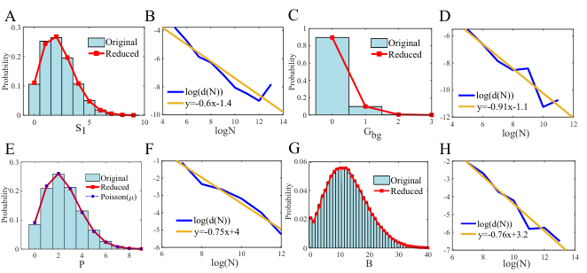
Both S1S_{1} and S4S_{4} in (42) follow a simple birth-death process and hence the stationary distribution of ZZ is a Poisson distribution so that the condition (17) holds. Furthermore, unlikely in the original model (41), probability densities of species S1S_{1} and S5S_{5} at time tt are analytically tractable as it is shown in [15] that the time evolution of the probabilities for a linear birth-death process is a convolution of Poisson distributions and multinomial distributions. Thus we can analytically approximate the dynamics of the species in SLS_{L} of the original system (41). Figure 2A displays the density function of S1S_{1} for ZN,−θ0​(10)Z^{N,-\theta_{0}}(10) and the reduced system Z⁡(10)Z(10) with N=100N=100. Figure 2B displays the accuracy of the approximation indicating the convergence rate in the scaling parameter NN as proved in Theorem 3.1.

5.2 Yeast Polarization

In this section, we consider a signal-transduction pathway (43), which was introduced in [11]. In the system, species GG, so-called ‘G-proten’, serves an important role in yeast polarization [24]. GG goes through a separation-dephosphorylation-rebind cycle, as the 5th,6th and 7th reactions describe in (43), respectively. And this cycle is activated by ligand-receptor binding.

∅⇌κ2/Nκ1/NR,L+R→κ3/NRL+L,RL→κ4/NR,,R​L+G→κ5Ga+Gb​gGa→κ6/NGd,Gd+Gb​g→κ7G,∅→κ8RL.\displaystyle\begin{split}&\emptyset\xrightleftharpoons[\kappa_{2}/N]{\kappa_{1}/N}R,\quad L+R\xrightarrow{\kappa_{3}/N}RL+L,\quad RL\xrightarrow{\kappa_{4}/N}R,,\\ &RL+G\xrightarrow{\kappa_{5}}G_{a}+G_{bg}\quad G_{a}\xrightarrow{\kappa_{6}/N}G_{d},\\ &G_{d}+G_{bg}\xrightarrow{\kappa_{7}}G,\quad\emptyset\xrightarrow{\kappa_{8}}RL.\end{split} (43)

We model this yeast polarization system with a multiscale stochastic mass-action system. Let NN be the scaling parameter. We suppose that the initial copies of ligand LL, protein GG and its subunit Gb​gG_{bg} are Θ⁡(1)\Theta(1), and other species have the copy numbers of order NN. More precisely, for a multiscale process XN​(t)X^{N}(t) associated with (43), we set XRN​(0)=N,XLN​(0)=2,XR​LN​(0)=N,XGN​(0)=5,XGαN​(0)=N,XGb​gN​(0)=5X^{N}_{R}(0)=N,X^{N}_{L}(0)=2,X^{N}_{RL}(0)=N,X^{N}_{G}(0)=5,X^{N}_{G_{\alpha}}(0)=N,X^{N}_{G_{bg}}(0)=5 and XGdN​(0)=NX^{N}_{G_{d}}(0)=N. As described in (43), we scale the rate constants (see the caption of Figure 2 for the values of κi\kappa_{i}’s). Then by computing the reaction intensities at XN​(0)X^{N}(0), we have the maximum order of reaction intensity θ0\theta_{0} and then we classify the reactions into ℛ0={yk→yk′:k=5,7}\mathcal{R}_{0}=\{y_{k}\to y^{\prime}_{k}:k=5,7\} and ℛ0c\mathcal{R}^{c}_{0}.

We approximate the scaled process ZN,−θ0​(t)Z^{N,-\theta_{0}}(t) under slow-timescale with the projected system (𝒮L,𝒞L,ℛL,𝒦L)(\mathcal{S}_{L},\mathcal{C}_{L},\mathcal{R}_{L},\mathcal{K}_{L}). The parameters sks_{k} defined around (16) are

s5=limN→∞λH,5N,−θ0=limN→∞N−θ0+β5+y5⋅α​ZR​LN,−θ0​(0)=1,\displaystyle s_{5}=\lim_{N\to\infty}\lambda^{N,-\theta_{0}}_{H,5}=\lim_{N\to\infty}N^{-\theta_{0}+\beta_{5}+y_{5}\cdot\alpha}Z^{N,-\theta_{0}}_{RL}(0)=1,
s7=limN→∞λH,7N,−θ0=limN→∞N−θ0+β7+y7⋅α​ZGdN,−θ0​(0)=1.\displaystyle s_{7}=\lim_{N\to\infty}\lambda^{N,-\theta_{0}}_{H,7}=\lim_{N\to\infty}N^{-\theta_{0}+\beta_{7}+y_{7}\cdot\alpha}Z^{N,-\theta_{0}}_{G_{d}}(0)=1.

Then the projected system is

G⇌κ7κ5Gb​g.\displaystyle G\xrightleftharpoons[\kappa_{7}]{\kappa_{5}}G_{bg}. (44)

The stochastic process Z⁡(t)=(ZG​(t),ZGb​g​(t))Z(t)=(Z_{G}(t),Z_{G_{bg}}(t)) associated with (44) admits a finite state space as the total quantity of GG and Gb​gG_{bg} is preserved. Hence (17) hold. Furthermore the probability density function can be analytically derived as p⁡(t)=μ​e−Q​tp(t)=\mu e^{-Qt} where QQ is the transition matrix of ZZ defined on {(z1,z2):z1+z2=ZG​(0)+ZGb​g​(0)=10}\{(z_{1},z_{2}):z_{1}+z_{2}=Z_{G}(0)+Z_{G_{bg}}(0)=10\} and μ\mu is the initial distribution of ZZ such that μ⁡(5,5)=1\mu(5,5)=1. We show model reduction in Figure 2CD with almost the same rate constants used in [11]. In Figure 2C, letting N=1000N=1000, we compare the probability densities of Gb​gG_{bg} of ZN,−θ0Z^{N,-\theta_{0}} associated with (43) and its reduced system ZZ associated with (44) at time t=10t=10. Figure 2D furthermore shows the convergence rate of the approximation.
Refer to caption
Figure 2: AB. Model reduction for the futile system (41). Parameters are κ3=0.1\kappa_{3}=0.1 and κ6=0.1\kappa_{6}=0.1, and κi=1\kappa_{i}=1 otherwise. The probability density of the original model is calculated with 10510^{5} times of Gillespie’s simulations [13]. A. Comparison of the distributions OPENP⁡(S1N,−θ0​(t)=zℓ))P(S^{N,-\theta_{0}}_{1}(t)=z_{\ell})) and P⁡(S1​(t)=zℓ)P(S_{1}(t)=z_{\ell}) at t=100t=100 with N=104N=10^{4}. B. Convergence d⁡(N)=|P⁡(ZN,−θ0​(t)∈A)−P⁡(Z⁡(t)∈A)|d(N)=|P(Z^{N,-\theta_{0}}(t)\in A)-P(Z(t)\in A)| as NN increases for A={S1=3 or 4}A=\{S_{1}=3\text{ or }4\} at t=100t=100. CD. Model reduction for the yeast polarization system (43). Parameters are κ1=3.8,κ2=40,κ3=42,κ4=10,κ5=0.011,κ6=10,κ7=1\kappa_{1}=3.8,\kappa_{2}=40,\kappa_{3}=42,\kappa_{4}=10,\kappa_{5}=0.011,\kappa_{6}=10,\kappa_{7}=1 and κ8=3.21\kappa_{8}=3.21. The probability density of the original model is calculated with 10710^{7} times of Gillespie’s simulations. C. Comparison of the distributions OPENP⁡(Gb​gN,−θ0​(t)=zℓ))P(G_{bg}^{N,-\theta_{0}}(t)=z_{\ell})) and P⁡(Gb​g​(t)=zℓ)P(G_{bg}(t)=z_{\ell}) at t=10t=10 with N=103N=10^{3}. D. Convergence of d⁡(N)=|P⁡(ZN,−θ0​(t)∈A)−P⁡(Z⁡(t)∈A)|d(N)=|P(Z^{N,-\theta_{0}}(t)\in A)-P(Z(t)\in A)| as NN increases for A={S1=3 or 4}A=\{S_{1}=3\text{ or }4\} at t=100t=100. EF. Model reduction for the system of p53 response (45). The parameters κi\kappa_{i} are 1.1,0.6,0.3,0.3,3.4,4.5,4.1,0.6,1.1,0.9,1.9,3.2,3.21.1,0.6,0.3,0.3,3.4,4.5,4.1,0.6,1.1,0.9,1.9,3.2,3.2, and 3.03.0 for i=1,2​…,14i=1,2\dots,14, respectively. Furthermore c1=4.7c_{1}=4.7 and c2=1.9c_{2}=1.9. Each parameter is sampled uniformly in [0,5][0,5]. 10710^{7} Gillespie’s simulations are used to estimate the probability densities of the original and reduced models. E. Comparison of the distributions OPENP⁡(P1N,−θ0​(t)=zℓ))P(P^{N,-\theta_{0}}_{1}(t)=z_{\ell})) and P⁡(P⁡(t)=zℓ)P(P(t)=z_{\ell}) at t=100t=100 with N=105N=10^{5}. F. Convergence d⁡(N)=|P⁡(PN,−θ0​(t)∈A)−P⁡(P⁡(t)∈A)|d(N)=|P(P^{N,-\theta_{0}}(t)\in A)-P(P(t)\in A)| as NN increases for A={P=3 or 4}A=\{P=3\text{ or }4\} at t=100t=100. GH. Model reduction for the population model (46). The parameters κi\kappa_{i} are 0.5,1.7,3.9,4.6,2.7,1.9,6.1,2.40.5,1.7,3.9,4.6,2.7,1.9,6.1,2.4, and 1.51.5 for i=1,2​…,9i=1,2\dots,9, respectively. Each parameter is sampled uniformly in [0,5][0,5]. We sampled 10510^{5} trajectories with Gillespie’s algorithm to estimate the probability densities of the original and reduced models. G. Comparison of the distributions OPENP⁡(BN,−θ0​(t)=zℓ))P(B^{N,-\theta_{0}}(t)=z_{\ell})) and P⁡(B⁡(t)=zℓ)P(B(t)=z_{\ell}) at t=150t=150 with N=105N=10^{5}. H. Convergence d⁡(N)=|P⁡(BN,−θ0​(t)∈U)−P⁡(B⁡(t)∈U)|d(N)=|P(B^{N,-\theta_{0}}(t)\in U)-P(B(t)\in U)| as NN increases for U={B≥10}U=\{B\geq 10\} at t=150t=150. The yellow straight lines in BDFH indicate that the convergence rate of d⁡(N)d(N) to 00 is in Θ⁡(1Nν)\Theta(\frac{1}{N^{\nu}}) for some ν∈(0,1)\nu\in(0,1).

5.3 p53 response to DNA damage

Network (45) describes signaling pathway and negative feedback for activating p53 proteins in damages DNA, which is introduced in [5]. When DNA is damages, signaling kinases (S) such as ATM and Chk2 convert inactive p53 protein (P0P_{0}) to active p53 protein (P). The p53 protein also represses itself by the negative feedback loop with the Mdm2 protein (M). Another negative feedback loop between p53, the signal and inhibitor (I) is also present in this system. See a schematic description of this system in [5, Figure 1B]

P0+S→N​κ1P+S,P0+M→κ2M,P+M→κ3M,P→κ4P+M,P→κ5P+I,S+M→κ6/NS,S+I→κ7I,P⇌N​κ9κ8∅⇌κ11κ10M,S⇌κ13κ12∅←κ14I.\displaystyle\begin{split}&P_{0}+S\xrightarrow{N\kappa_{1}}P+S,\\ &P_{0}+M\xrightarrow{\kappa_{2}}M,\quad\ \ \ \ \qquad P+M\xrightarrow{\kappa_{3}}M,\\ &P\xrightarrow{\kappa_{4}}P+M,\quad\ \ \ \ \ \qquad P\xrightarrow{\kappa_{5}}P+I,\\ &S+M\xrightarrow{\kappa_{6}/N}S,\quad\ \ \qquad S+I\xrightarrow{\kappa_{7}}I,\\ &P\xrightleftharpoons[N\kappa_{9}]{\kappa_{8}}\emptyset\xrightleftharpoons[\kappa_{11}]{\kappa_{10}}M,\quad\qquad S\xrightleftharpoons[\kappa_{13}]{\kappa_{12}}\emptyset\xleftarrow{\kappa_{14}}I.\end{split} (45)

To match the initial setting used in [5], we assume that the inhibitor has low copies at the beginning. Furthermore we assume that P0P_{0} and PP have also initially low copies. Precisely, XP0N​(0)=5,XP0N​(0)=0,XIN​(0)=1,XNN​(0)=NX^{N}_{P_{0}}(0)=5,X^{N}_{P_{0}}(0)=0,X^{N}_{I}(0)=1,X^{N}_{N}(0)=N and XSN​(0)=5​NX^{N}_{S}(0)=5N. Hence 𝒮L={P0,P,I}\mathcal{S}_{L}=\{P_{0},P,I\} and 𝒮H={M,S}\mathcal{S}_{H}=\{M,S\}. For each state x=(xP0,xP,xS,xM,xI)x=(x_{P_{0}},x_{P},x_{S},x_{M},x_{I}), the reaction intensities λ1\lambda_{1} and λ7\lambda_{7} contain hill-functions as

λ1​(x)=N​κ1​xP0​xSxS+c1,andλ7​(x)=κ7​xS​xIxI+c2,\displaystyle\lambda_{1}(x)=N\kappa_{1}x_{P_{0}}\frac{x_{S}}{x_{S}+c_{1}},\quad\text{and}\quad\lambda_{7}(x)=\kappa_{7}x_{S}\frac{x_{I}}{x_{I}+c_{2}},

for some positive constants c1c_{1} and c2c_{2}. The other intensities follow the mass-action kinetics (5). Under the scaled rate constants shown in (45). Then the maximum order θ0\theta_{0} of the intensities is 11 so that ℛ0\mathcal{R}_{0} contains reaction 1,2,3,6,7,9,111,2,3,6,7,9,11 and 1212. For the process ZN,−θ0​(t)Z^{N,-\theta_{0}}(t) under slow-timescale, the associated projected network (𝒮L,𝒞L,ℛL,𝒦L)(\mathcal{S}_{L},\mathcal{C}_{L},\mathcal{R}_{L},\mathcal{K}_{L}) is

P0→s1​κ1P\displaystyle\quad P_{0}\xrightarrow{\ \hskip 8.19447pts_{1}\kappa_{1}\hskip 8.19447pt\ }P
s8​κ8↘↖s2​κ2↙s3​κ3\displaystyle\text{\footnotesize{$s_{8}\kappa_{8}$}}\searrow\hskip-14.22636pt\nwarrow\text{\footnotesize{$\ s_{2}\kappa_{2}$}}\hskip 11.38092pt\swarrow\hskip-5.69046pt\text{\footnotesize{$s_{3}\kappa_{3}$}}
∅\displaystyle\hskip 39.83368pt\emptyset

where the parameters sks_{k}’s are defined as in (16). Especially for the non-mass action intensity λ1N​(ZN,−θ0​(0))\lambda^{N}_{1}(Z^{N,-\theta_{0}}(0)) we have

s1=limN→∞λH,1N,−θ0​(qH​(ZN,−θ0​(0))=N−θ0+β1​NN+c1=1CLOSE.\displaystyle s_{1}=\lim_{N\to\infty}\lambda^{N,-\theta_{0}}_{H,1}(q_{H}(Z^{N,-\theta_{0}}(0))=N^{-\theta_{0}+\beta_{1}}\frac{N}{N+c_{1}}=1.

Note that these intensities under non-mass action kinetics satisfy (CD1)–(CD3). Let Z⁡(t)Z(t) be the stochastic process associated with (𝒮L,𝒞L,ℛL,𝒦L)(\mathcal{S}_{L},\mathcal{C}_{L},\mathcal{R}_{L},\mathcal{K}_{L}). The time evolution of the probability density of Z⁡(t)Z(t) is analytically intractable. However, it can be shown that the probability density converges to a unique stationary distribution, which can be explicitly derived. (𝒮L,𝒞L,ℛL,𝒦L)(\mathcal{S}_{L},\mathcal{C}_{L},\mathcal{R}_{L},\mathcal{K}_{L}) satisfies special network structure, so-called zero deficiency and weakly reversible, and hence its stationary distribution is a product form of Poisson distributions [2, Theorem 6.1]. See Appendix for more details.

Figure 2E displays the probability distribution of the original and reduced models along with Poisson distribution of rate μ=2.4\mu=2.4, which is the average of PP in (𝒮L,𝒞L,ℝL,𝒦L)(\mathcal{S}_{L},\mathcal{C}_{L},\mathbb{R}_{L},\mathcal{K}_{L}). A commodity machine was used to simulate the samples in parallel (parfor in Matlab with 6 workers) and took 317 sec for the original model and 2.4 sec for the reduced model. We also show the convergence of the original model in Figure 2E.

5.4 Three species Lotka-Volterra model with migration

We consider a multiscale Lotka-Volterra population model (46) with the scailing parameter NN. There exists three species in the network where AA is the lowest level prey, BB is the middle level species, and CC is the top level predator.

B⇌κ2κ1∅,A⇌κ4κ3/N∅,C⇌κ6κ5∅,A→κ7/N2A,A+B→κ8/N2B,B+C→κ92C.\displaystyle\begin{split}&B\xrightleftharpoons[\kappa_{2}]{\kappa_{1}}\emptyset,\quad A\xrightleftharpoons[\kappa_{4}]{\kappa_{3}/N}\emptyset,\quad C\xrightleftharpoons[\kappa_{6}]{\kappa_{5}}\emptyset,\\ &A\xrightarrow{\kappa_{7}/N}2A,\quad A+B\xrightarrow{\kappa_{8}/N}2B,\quad B+C\xrightarrow{\kappa_{9}}2C.\end{split} (46)

We use non-mass action kinetics for the reactions A+B→2​BA+B\to 2B and B+C→2​CB+C\to 2C to model ‘weak hunting’ of BB and CC such that for each x=(xA,xB,xC)x=(x_{A},x_{B},x_{C}),

λ8​(x)=κ8N​xA​xBandλ9​(x)=κ9​log⁡(xB​xC+1).\displaystyle\lambda_{8}(x)=\frac{\kappa_{8}}{N}x_{A}\sqrt{x_{B}}\quad\text{and}\quad\lambda_{9}(x)=\kappa_{9}\log(x_{B}x_{C}+1).

The other reaction intensities obey the mass-action kinetics. We assume that 𝒮L={B,C}\mathcal{S}_{L}=\{B,C\} and 𝒮H={A}\mathcal{S}_{H}=\{A\} as XAN​(0)=NX^{N}_{A}(0)=N, XBN​(0)=10X^{N}_{B}(0)=10 and XCN​(0)=10X^{N}_{C}(0)=10. Under the scaled rate constants shown in (46), the maximum order of the reaction intensities θ0\theta_{0} is 00, and every reaction belongs to ℛ0\mathcal{R}_{0}. Note that we assumed that slow birth and slow degradation of AA so that the associated reaction rate constants for the 3rd and 7th reactions are of order 1N\frac{1}{N}.

For the scaled process ZN,−θ0​(t)Z^{N,-\theta_{0}}(t), the scaled reaction intensities are decomposed as defined in (15), especially for each z=(zA,zB,zC)z=(z_{A},z_{B},z_{C}) λH,8N,−θ0=Nβ8+y8⋅α​zA,λL,8=κ8​zB\lambda^{N,-\theta_{0}}_{H,8}=N^{\beta_{8}+y_{8}\cdot\alpha}z_{A},\lambda_{L,8}=\kappa_{8}\sqrt{z_{B}}, λH,9N,−θ0=1\lambda^{N,-\theta_{0}}_{H,9}=1 and λL,9=κ9​log⁡(zB​zC+1)\lambda_{L,9}=\kappa_{9}\log(z_{B}z_{C}+1). Hence (CD1)–(CD3) hold.

Now we consider the projected system. As the the reaction A+B→2​BA+B\to 2B obeys non-mass action kinetics involving A∈𝒮HA\in\mathcal{S}_{H}, parameter the s8s_{8} is especially computed as s8=limN→∞λH,8N​(ZN,−θ0​(0))=1s_{8}=\lim_{N\to\infty}\lambda^{N}_{H,8}(Z^{N,-\theta_{0}}(0))=1. Hence the projected system is

B⇌κ2κ1∅,C⇌κ6κ5∅B→κ82​B,B+C→κ92​C.\displaystyle B\xrightleftharpoons[\kappa_{2}]{\kappa_{1}}\emptyset,\quad C\xrightleftharpoons[\kappa_{6}]{\kappa_{5}}\emptyset\quad B\xrightarrow{\kappa_{8}}2B,\quad B+C\xrightarrow{\kappa_{9}}2C. (47)

Let Z⁡(t)Z(t) be the stochastic process associated with (47) In Appendix, we show how to use the Foster-Lyapunov criterion [23] to verify that a stationary distribution π\pi of ZZ exists and how π\pi meets the condition (17). The approximation and convergence rates of species BB is shown in Figure 2G and H. A commodity machine was used to approximate the probability densities in parallel (parfor in Matlab with 6 workers) and took 174 sec for the original model and 70 sec for the reduced model.

6 Discussion

When a stochastic biochemical reaction system contains species with different orders of abundance, one can model the system using a multiscaling approach. We have shown in this paper that a multiscale stochastic reaction a short-term timescale can be approximated using a reduced stochastic system with a specific error bound.

The scaling regime we considered in this paper is a special case of the scaling under the so-called species balance condition, which was introduced in [17]. More general multiscaling limits of stochastic reactions introduced by Kurtz and others rely on the law of large numbers and relative compactness of probability measures in a metric spaces [1, 4, 17, 21]. This general framework covers a wide range of multiscaling limits, but the convergence rate in the general case remains unknown. Instead of the classical methods, here we have used a direct analysis of the Kolmogorov forward equation, and we also use the state space truncation through FSP to exploit the distance between two probability measures more explicitly.

One of the key steps for the main result was to show that the concentrations of the order NN species are confined near the initial concentrations. To do this, we showed that the multiscale model is non-explosive by assuming that the reduced system admits a stationary distribution satisfying a finite moment condition. Indeed, this assumption implies the tightness of the family of multiscale stochastic processes, which in turn implies the relative compactness of the sequence of probability measures. This assumption is also closely related to some technical conditions on stoichiometric coefficients such as the binary or unary conditions assumed in [1, 17].

We can generalize the rate of the convergence in the main result if all the moments of the stationary distribution π\pi in 17 are finite. Based on a suggestion by Chaojie Yuan for this case, we used the Burkholder–Davis–Gundy inequality [6] and were able to prove inductively the alternative result that E⁡(J​(t)m)≤c​tmE(J(t)^{m})\leq ct^{m} in Lemma 3.3. By combining this result with the other lemmas with slight modifications, it follows that

|pN​(A,ℝ≥0r,t)−p⁡(A,t)|≤c​max⁡{1,tm}Nνfor any ν∈(0,1).\displaystyle|p^{N}(A,\mathbb{R}^{r}_{\geq 0},t)-p(A,t)|\leq\frac{c\max\{1,t^{m}\}}{N^{\nu}}\quad\text{for any $\nu\in(0,1)$}.

The main result in this paper can shed light on the applicability of multiscaling model approximations for the analysis of stochastic reaction systems. In the analysis that we proposed for the multiscale model reduction, the convergence of the probability measure has been exhibited more explicitly than in the existing literature. The main result can also strengthen the applicability of this theoretical framework to practical problems in systems biology such as rational circuit design and the study of absolute robustness [20].

Acknowledgment

We would like to thank Eduardo Sontag, Carsten Wiuf, Chuang Xu and Linard Hoessly for key suggestions regarding this work, as well as Chaojie Yuan for an alternative proof of an important lemma.

Appendix A: Table of symbols

Symbol Meaning
𝒮,𝒞,ℛ\mathcal{S},\mathcal{C},\mathcal{R} and 𝒦\mathcal{K} Set of species, complexes, reaction and reaction intensities, respectively
Xi​(t)X_{i}(t) The count of ii th species at time tt
XN​(t)X^{N}(t) A multiscale stochastic model associated with a reaction network
ZN,γ​(t)Z^{N,\gamma}(t) A scaled process
dd Number of species of low initial copies
rr Number of species of high initial copies
ℤ≥0d\mathbb{Z}^{d}_{\geq 0} {x∈ℤd:xi≥0​ for each i}\{x\in\mathbb{Z}^{d}:x_{i}\geq 0\text{ for each $i$}\}
ℛ≥0r\mathcal{R}^{r}_{\geq 0} {z∈ℝr:zi≥0​ for each i}\{z\in\mathbb{R}^{r}:z_{i}\geq 0\text{ for each $i$}\}
pN​(⋅,t)p^{N}(\cdot,t) Probability density function of ZN,−θ0​(t)Z^{N,-\theta_{0}}(t)
p⁡(⋅,t)p(\cdot,t) Probability density function of Z⁡(t)Z(t)
n(k)n^{(k)} n(n−1)⋯(n−k+1)𝟙n≥kn(n-1)\cdots(n-k+1)\mathbbm{1}_{n\geq k} for non-negative integers nn and kk
u(v)u^{(v)} ∏i=1dui(vi)\prod_{i=1}^{d}u_{i}^{(v_{i})} for u,v∈ℤ≥0du,v\in\mathbb{Z}^{d}_{\geq 0}
uvu^{v} ∏i=1duivi\prod_{i=1}^{d}u_{i}^{v_{i}} for u,v∈ℝ≥0du,v\in\mathbb{R}^{d}_{\geq 0}
𝒮L\mathcal{S}_{L} Set of species such that Xi​(0)=Θ​(1)X_{i}(0)=\Theta(1)
𝒮H\mathcal{S}_{H} Set of species such that Xi​(0)=Θ​(N)X_{i}(0)=\Theta(N)
λk\lambda_{k} Reaction intensity of XNX^{N} associated with the kk th reaction.
λkN,γ\lambda^{N,\gamma}_{k} Reaction intensity of ZN,γZ^{N,\gamma} associated with the kk th reaction (11).
λL,k\lambda_{L,k}, λH,kN,γ\lambda^{N,\gamma}_{H,k} Decomposition of λkN,γ\lambda^{N,\gamma}_{k} (15).
y′N−yN{y^{\prime}}^{N}-y^{N} The scaled reaction vector with the ii th component yk,i′−yk,iNαi\frac{y^{\prime}_{k,i}-y_{k,i}}{N^{\alpha_{i}}}

Appendix B: Proof of Lemmas in Section 3.2

Proof of Lemma 3.2.

Suppose first that yk→yk′∈ℛ0y_{k}\to y^{\prime}_{k}\in\mathcal{R}_{0}. As defined in (15), we use the decomposition of λkN,−θ0​(z)=κk​λL,k​(zℓ)​λH,kN,−θ0​(zh)\lambda^{N,-\theta_{0}}_{k}(z)=\kappa_{k}\lambda_{L,k}(z_{\ell})\lambda^{N,-\theta_{0}}_{H,k}(z_{h}). As we discussed in Remark 2.2, the intensities of ZZ can be calculated as λ¯u​(zℓ)=κ¯u​(zℓ)(y¯u)=κ¯u​λL,k​(zℓ)\bar{\lambda}_{u}(z_{\ell})=\bar{\kappa}_{u}(z_{\ell})^{(\bar{y}_{u})}=\bar{\kappa}_{u}\lambda_{L,k}(z_{\ell}) if qL​(yk)=y¯uq_{L}(y_{k})=\bar{y}_{u}. Hence by definition of SMS_{M} in (20),

|λkN,−θ0​(z)−sk​κkκ¯u​λ¯u​(zℓ)|=κk​λL,k​(zℓ)​|λH,kN,−θ0​(zh)−sk|≤κk​λL,k​MN=κk​λL,k​1N1−ρ,\displaystyle\begin{split}\left|\lambda^{N,-\theta_{0}}_{k}(z)-\frac{s_{k}\kappa_{k}}{\bar{\kappa}_{u}}\bar{\lambda}_{u}(z_{\ell})\right|&=\kappa_{k}\lambda_{L,k}(z_{\ell})\left|\lambda^{N,-\theta_{0}}_{H,k}(z_{h})-s_{k}\right|\\ &\leq\kappa_{k}\lambda_{L,k}\frac{M}{N}=\kappa_{k}\lambda_{L,k}\frac{1}{N^{1-\rho}},\end{split} (48)

for each z∈SMz\in S_{M}. Therefore (i) follows with ν1=1−ρ\nu_{1}=1-\rho.

To show (ii), we recall that −θ0+βk+yk⋅α<0-\theta_{0}+\beta_{k}+y_{k}\cdot\alpha<0 for each yk→yk′∈ℛ0cy_{k}\to y_{k}^{\prime}\in\mathcal{R}^{c}_{0}, which implies that for ZN,−θ0​(0)=z0Z^{N,-\theta_{0}}(0)=z^{0}

sk=limN→∞N−θ0+βk+yk⋅α∏i=d+1d+rzi0(zi0−1N)⋯(zi0−yi−1N)=0.\displaystyle s_{k}=\lim_{N\to\infty}N^{-\theta_{0}+\beta_{k}+y_{k}\cdot\alpha}\prod_{i=d+1}^{d+r}z^{0}_{i}\left(z^{0}_{i}-\frac{1}{N}\right)\cdots\left(z^{0}_{i}-\frac{y_{i}-1}{N}\right)=0.

Thus (ii) follows with ν2=1−ρ⁡(maxk⁡‖qL​(yk)‖∞+1)\nu_{2}=1-\rho(\max_{k}\|q_{L}(y_{k})\|_{\infty}+1) by choosing sufficiently small ρ∈(0,1)\rho\in(0,1) for M=NρM=N^{\rho} because for z∈SMz\in S_{M}

λkN,−θ0​(z)≤κk​λL,k⁡(zℓ)​MN≤κk​M‖qL​(yk)‖∞​MN=κk​1Nν2.\displaystyle\lambda^{N,-\theta_{0}}_{k}(z)\leq\kappa_{k}\lambda_{L,k(z_{\ell})}\frac{M}{N}\leq\kappa_{k}M^{\|q_{L}(y_{k})\|_{\infty}}\frac{M}{N}=\kappa_{k}\frac{1}{N^{\nu_{2}}}.

Lastly, to show that (iii) we note that ∑y→y′∈ℛ0sk​κk​λL,k​(z)=∑uκu​λ¯u​(z)\displaystyle\sum\limits_{y\to y^{\prime}\in\mathcal{R}_{0}}s_{k}\kappa_{k}\lambda_{L,k}(z)=\sum_{u}\kappa_{u}\bar{\lambda}_{u}(z). Then by (i) and (ii) there exists c>0c>0 such that for any z∈SMz\in S_{M}

∑kλkN,−θ0​(z)\displaystyle\sum_{k}\lambda^{N,-\theta_{0}}_{k}(z) =∑yk→yk′∈ℛ0λkN,−θ0​(z)+∑yk→yk′∈ℛ0cλkN,−θ0​(z)\displaystyle=\sum_{y_{k}\to y_{k}^{\prime}\in\mathcal{R}_{0}}\lambda^{N,-\theta_{0}}_{k}(z)+\sum_{y_{k}\to y_{k}^{\prime}\in\mathcal{R}^{c}_{0}}\lambda^{N,-\theta_{0}}_{k}(z)
≤∑yk→yk′∈ℛ0|λkN,−θ0​(z)−sk​κkκ¯u​λ¯u​(zℓ)|+∑yk→yk′∈ℛ0sk​κkκ¯u​λ¯u​(zℓ)\displaystyle\leq\sum_{y_{k}\to y_{k}^{\prime}\in\mathcal{R}_{0}}\left|\lambda^{N,-\theta_{0}}_{k}(z)-\frac{s_{k}\kappa_{k}}{\bar{\kappa}_{u}}\bar{\lambda}_{u}(z_{\ell})\right|+\sum_{y_{k}\to y_{k}^{\prime}\in\mathcal{R}_{0}}\frac{s_{k}\kappa_{k}}{\bar{\kappa}_{u}}\bar{\lambda}_{u}(z_{\ell})
+∑yk→yk′∈ℛ0cλkN,−θ0(z)\displaystyle\ \ \ +\sum_{y_{k}\to y_{k}^{\prime}\in\mathcal{R}^{c}_{0}}\lambda^{N,-\theta_{0}}_{k}(z)
≤∑yk→yk′∈ℛ0κk​λL,k​(zℓ)Nν1+∑yk→yk′∈ℛ0sk​κkκ¯u​λ¯u​(zℓ)+cNν2\displaystyle\leq\sum_{y_{k}\to y_{k}^{\prime}\in\mathcal{R}_{0}}\frac{\kappa_{k}\lambda_{L,k}(z_{\ell})}{N^{\nu_{1}}}+\sum_{y_{k}\to y_{k}^{\prime}\in\mathcal{R}_{0}}\frac{s_{k}\kappa_{k}}{\bar{\kappa}_{u}}\bar{\lambda}_{u}(z_{\ell})+\frac{c}{N^{\nu_{2}}}
≤cNν1​∑uλ¯u​(zℓ)+∑uλ¯u​(zℓ)+cNν2=(1+cNν1)​∑uλ¯u​(zℓ)+cNν2.\displaystyle\leq\frac{c}{N^{\nu_{1}}}\sum_{u}\bar{\lambda}_{u}(z_{\ell})+\sum_{u}\bar{\lambda}_{u}(z_{\ell})+\frac{c}{N^{\nu_{2}}}=\left(1+\frac{c}{N^{\nu_{1}}}\right)\sum_{u}\bar{\lambda}_{u}(z_{\ell})+\frac{c}{N^{\nu_{2}}}.

Then by (21), the upper bound of ∑kλkN,−θ0​(z)\sum_{k}\lambda^{N,-\theta_{0}}_{k}(z) follows. The lower bound also holds as

∑kλkN,−θ0​(z)\displaystyle\sum_{k}\lambda^{N,-\theta_{0}}_{k}(z) ≥∑yk→yk′∈ℛ0λkN,−θ0​(z)\displaystyle\geq\sum_{y_{k}\to y_{k}^{\prime}\in\mathcal{R}_{0}}\lambda^{N,-\theta_{0}}_{k}(z)
≥∑yk→yk′∈ℛ0(λkN,−θ0​(z)−sk​κkκ¯u​λ¯u​(zℓ))+∑yk→yk′∈ℛ0sk​κkκ¯u​λ¯u​(zℓ)\displaystyle\geq\sum_{y_{k}\to y_{k}^{\prime}\in\mathcal{R}_{0}}\left(\lambda^{N,-\theta_{0}}_{k}(z)-\frac{s_{k}\kappa_{k}}{\bar{\kappa}_{u}}\bar{\lambda}_{u}(z_{\ell})\right)+\sum_{y_{k}\to y_{k}^{\prime}\in\mathcal{R}_{0}}\frac{s_{k}\kappa_{k}}{\bar{\kappa}_{u}}\bar{\lambda}_{u}(z_{\ell})
≥−∑yk→yk′∈ℛ0κk​λL,k​(zℓ)Nν1+∑yk→yk′∈ℛ0sk​κkκ¯uλ¯u(zℓ)\displaystyle\geq-\sum_{y_{k}\to y_{k}^{\prime}\in\mathcal{R}_{0}}\frac{\kappa_{k}\lambda_{L,k}(z_{\ell})}{N^{\nu_{1}}}+\sum_{y_{k}\to y_{k}^{\prime}\in\mathcal{R}_{0}}\frac{s_{k}\kappa_{k}}{\bar{\kappa}_{u}}\bar{\lambda}_{u}(z_{\ell})
≥(−cNν1+1)​∑uλ¯u​(zℓ)\displaystyle\geq\left(-\frac{c}{N^{\nu_{1}}}+1\right)\sum_{u}\bar{\lambda}_{u}(z_{\ell})

∎

Proof of Lemma 3.3.

By the random-time representation (6),
J⁡(t)=∑y¯u→y¯u′∈ℛLYu​(∫0tλ¯u​(Z⁡(s))​𝑑s)J(t)=\displaystyle\sum\limits_{\bar{y}_{u}\to\bar{y}^{\prime}_{u}\in\mathcal{R}_{L}}Y_{u}\left(\displaystyle\int_{0}^{t}\bar{\lambda}_{u}(Z(s))ds\right), where YuY_{u} are independent unit Poisson random variables. Note that for each uu,

Yu​(∫0tλ¯u​(Z⁡(s))​𝑑s)−∫0tλ¯u​(Z⁡(s))​𝑑s\displaystyle Y_{u}\left(\int_{0}^{t}\bar{\lambda}_{u}(Z(s))ds\right)-\int_{0}^{t}\bar{\lambda}_{u}(Z(s))ds

is a Martingale process [3]. We denote by Mu​(t)M_{u}(t) this Martingale. Then the quadratic variation of Mu​(t)M_{u}(t) is [Mu]​(t)=Yu​(∫0tλ¯u​(Z⁡(s))​𝑑s)[M_{u}](t)=Y_{u}\left(\int_{0}^{t}\bar{\lambda}_{u}(Z(s))ds\right). Since Mu2​(t)−[Mu]​(t)M^{2}_{u}(t)-[M_{u}](t) is a martingale [3], we have that by using Jansen’s inequality

E⁡(Yu​(∫0tλ¯u​(Z⁡(s))​𝑑s)2)\displaystyle E\left(Y_{u}\left(\int_{0}^{t}\bar{\lambda}_{u}(Z(s))ds\right)^{2}\right) ≤2​E​(Mu​(t)2)+2​E​((∫0tλ¯u​(Z⁡(s))​𝑑s)2)\displaystyle\leq 2E(M_{u}(t)^{2})+2E\left(\left(\int_{0}^{t}\bar{\lambda}_{u}(Z(s))ds\right)^{2}\right)
≤2​E​([Mu]​(t))+2​t​E​(∫0tλ¯u​(Z⁡(s))2​𝑑s)\displaystyle\leq 2E([M_{u}](t))+2tE\left(\int_{0}^{t}\bar{\lambda}_{u}(Z(s))^{2}ds\right) (49)

For a fixed initial value Z⁡(0)=z0Z(0)=z^{0}, there exists c>0c>0 such that P⁡(Z⁡(s)=z)≤c​π​(z)P(Z(s)=z)\leq c\pi(z) for any zz because

π⁡(z)=∑xP⁡(Z⁡(s)=z|Z⁡(0)=x)​π​(x)≥P⁡(Z⁡(s)=z)​π​(z0).\displaystyle\pi(z)=\sum_{x}P(Z(s)=z\ |\ Z(0)=x)\pi(x)\geq P(Z(s)=z)\pi(z^{0}).

This implies that by 17, we have

E​([Mu]​(t))\displaystyle E([M_{u}](t)) =E⁡(Yu​(∫0tλ¯u​(Z⁡(s))))=∫0t∑x∑uλ¯u​(x)​P​(Z⁡(s)=x)​𝑑s\displaystyle=E\left(Y_{u}\left(\int_{0}^{t}\bar{\lambda}_{u}(Z(s))\right)\right)=\int_{0}^{t}\sum_{x}\sum_{u}\bar{\lambda}_{u}(x)P(Z(s)=x)ds
≤c1​∑xλ¯u​(x)​π​(x)​t≤c1′​t,\displaystyle\leq c_{1}\sum_{x}\bar{\lambda}_{u}(x)\pi(x)t\leq c^{\prime}_{1}t,

with some positive constants c1c_{1} and c1′c^{\prime}_{1}. Similarly,

E⁡(∫0tλ¯u​(Z⁡(s))2​𝑑s)\displaystyle E\left(\int_{0}^{t}\bar{\lambda}_{u}(Z(s))^{2}ds\right) =∫0t∑xλ¯u​(x)2​P​(X⁡(s)=x)​𝑑s\displaystyle=\int_{0}^{t}\sum_{x}\bar{\lambda}_{u}(x)^{2}P(X(s)=x)ds
≤c2′​∫0t∑xλ¯u​(x)2​π​(x)​𝑑s≤c2​t,\displaystyle\leq c^{\prime}_{2}\int_{0}^{t}\sum_{x}\bar{\lambda}_{u}(x)^{2}\pi(x)ds\leq c_{2}t,

with some positive constants c2c_{2} and c2′c^{\prime}_{2}. Applying these to (49), it follows that

E⁡(Yu​(∫0tλ¯u​(Z⁡(s))​𝑑s)2)≤c′​max​{1,t2},\displaystyle E\left(Y_{u}\left(\int_{0}^{t}\bar{\lambda}_{u}(Z(s))ds\right)^{2}\right)\leq c^{\prime}\max\{1,t^{2}\},

with some positive constant c′c^{\prime}.

Finally the result follows since by Jansen’s inequality we have that there exists a positive constant cc such that

E⁡(J​(t)2)≤|ℛL|∑uE⁡((Yu​(∫0tλ¯u​(Z⁡(s))​𝑑s))2)≤c​max​{1,t2},\displaystyle E(J(t)^{2})\leq|\mathcal{R}_{L}|\sum_{u}E\left(\left(Y_{u}\left(\int_{0}^{t}\bar{\lambda}_{u}(Z(s))ds\right)\right)^{2}\right)\leq c\max\{1,t^{2}\},

∎

Proof of Lemma 3.4.

It is suffice to show that at least c​McM transitions are required for ZN,−θ0​(t)Z^{N,-\theta_{0}}(t) to escape SMS_{M}. Let ZN,−θ0​(0)=z0Z^{N,-\theta_{0}}(0)=z^{0} be the initial state. We first show that {zh:|zh−zh0|<c​MN}⊆SH,M\{z_{h}:|z_{h}-z^{0}_{h}|<c\frac{M}{N}\}\subseteq S_{H,M} for some c>0c>0. Note that if yk→yk′∈ℛ0y_{k}\to y_{k}^{\prime}\in\mathcal{R}_{0}, then sk=(zh0)qH​(yk)s_{k}=(z^{0}_{h})^{q_{H}(y_{k})} and −θ0+βk+yk⋅α=0-\theta_{0}+\beta_{k}+y_{k}\cdot\alpha=0. Then there exist c′>0c^{\prime}>0 and c′′>0c^{\prime\prime}>0 such that for any yk→yk′∈ℛ0y_{k}\to y_{k}^{\prime}\in\mathcal{R}_{0} if zh=zh0+ηz_{h}=z^{0}_{h}+\eta with |η|≤c′​MN|\eta|\leq c^{\prime}\frac{M}{N}, then

|zhqH​(yk)−sk|=|(zh0+η)qH​(yk)−sk|≤c′′​|η|≤M2​N,and\displaystyle|z_{h}^{q_{H}(y_{k})}-s_{k}|=|(z^{0}_{h}+\eta)^{q_{H}(y_{k})}-s_{k}|\leq c^{\prime\prime}|\eta|\leq\frac{M}{2N},\quad\text{and}
|zhqH​(yk)−λH,kN,−θ0(zh)|=|∏i=1rzh,iyk,d+i−∏i=1rzh,i(zh,i−1N)⋯(zh,i−yk,d+i−1N)|\displaystyle\left|z_{h}^{q_{H}(y_{k})}-\lambda^{N,-\theta_{0}}_{H,k}(z_{h})\right|=\left|\prod_{i=1}^{r}z_{h,i}^{y_{k,d+i}}-\prod_{i=1}^{r}z_{h,i}\left(z_{h,i}-\frac{1}{N}\right)\cdots\left(z_{h,i}-\frac{y_{k,d+i}-1}{N}\right)\right|
≤c′′N.\displaystyle\hskip 99.58464pt\leq\frac{c^{\prime\prime}}{N}.

This implies that for yk→yk′∈ℛ0y_{k}\to y^{\prime}_{k}\in\mathcal{R}_{0} if |zh−zh0|≤c′​MN|z_{h}-z^{0}_{h}|\leq c^{\prime}\frac{M}{N} then

|λH,kN,−θ0​(zh)−sk|≤|zhqH​(yk)−sk|+|zhqH​(yk)−λH,kN,−θ0​(zh)|≤MN,\displaystyle\left|\lambda^{N,-\theta_{0}}_{H,k}(z_{h})-s_{k}\right|\leq\left|z_{h}^{q_{H}(y_{k})}-s_{k}\right|+\left|z_{h}^{q_{H}(y_{k})}-\lambda^{N,-\theta_{0}}_{H,k}(z_{h})\right|\leq\frac{M}{N},

for sufficiently large NN. Hence {zh:|zh−zh0|<c​MN}⊆SH,M\{z_{h}:|z_{h}-z^{0}_{h}|<c\frac{M}{N}\}\subseteq S_{H,M}. Furthermore {zℓ:|zℓ−zℓ0|≤c′′′​M}⊆SL,M\{z_{\ell}:|z_{\ell}-z^{0}_{\ell}|\leq c^{\prime\prime\prime}M\}\subseteq S_{L,M} for some c′′′>0c^{\prime\prime\prime}>0 when NN is sufficiently large. Therefore

{zℓ:|zℓ−zℓ0|≤c′​M}×{zh:|zh−zh0|<c′′′​MN}⊂SM.\displaystyle\{z_{\ell}:|z_{\ell}-z^{0}_{\ell}|\leq c^{\prime}M\}\times\left\{z_{h}:|z_{h}-z^{0}_{h}|<c^{\prime\prime\prime}\frac{M}{N}\right\}\subset S_{M}.

Since the transition size for each entry ZiN,−θ0Z^{N,-\theta_{0}}_{i} of the scaled process transitions by a single reaction is Θ⁡(N−αi)\Theta(N^{-\alpha_{i}}), this implies that ZN,−θ0​(t)Z^{N,-\theta_{0}}(t) needs at least ⌊c​M⌋\lfloor cM\rfloor transitions for some c>0c>0 to escape SMS_{M}. ∎

Proof of Lemma 3.6.

dd​t​v​(t)≤A​v​(t)+b\frac{d}{dt}v(t)\leq Av(t)+b can be written as

v⁡(t)≤t​b+∫0tA​v​(s)​𝑑s\displaystyle v(t)\leq tb+\int_{0}^{t}Av(s)ds

allowing that the inequality holds component-wisely. Then by the multivariable Gronwall’s inequality [10],

v⁡(t)≤t​b+t​∫stV⁡(t,s)​A​b​𝑑s,\displaystyle v(t)\leq tb+t\int_{s}^{t}V(t,s)Abds,

where V⁡(t,s)V(t,s) satisfies

V⁡(t,s)=I+∫stA​V​(x,s)​𝑑x,\displaystyle V(t,s)=I+\int_{s}^{t}AV(x,s)dx,

allowing the equality holds component-wisely. By taking time-derivative, we notice that ii th column of V⁡(t,s)V(t,s) is a solution uu of the system of differential equation (32) with ui​(s)=1u_{i}(s)=1 and uj​(s)=0u_{j}(s)=0 if j≠ij\neq i. Therefore by the hypothesis in the statement, each column of V⁡(t,s)V(t,s) is a positive vector and the sum of the entries is equal to 11 for t≥st\geq s. Hence it implies that V⁡(t,s)​A​b≤A¯​bV(t,s)Ab\leq\bar{A}b for t≥st\geq s. Thus for each tt, the result follows. ∎

References

  • [1] David F Anderson, Daniele Cappelletti, and Thomas G Kurtz. Finite time distributions of stochastically modeled chemical systems with absolute concentration robustness. SIAM Journal on Applied Dynamical Systems, 16(3):1309–1339, 2017.
  • [2] David F. Anderson, Gheorghe Craciun, and Thomas G. Kurtz. Product-form stationary distributions for deficiency zero chemical reaction networks. Bull. Math. Biol., 72(8):1947–1970, 2010.
  • [3] David F. Anderson and Thomas G Kurtz. Continuous time Markov chain models for chemical reaction networks. In H Koeppl Et al., editor, Design and Analysis of Biomolecular Circuits: Engineering Approaches to Systems and Synthetic Biology, pages 3–42. Springer, 2011.
  • [4] Karen Ball, Thomas G Kurtz, Lea Popovic, Greg Rempala, et al. Asymptotic analysis of multiscale approximations to reaction networks. The Annals of Applied Probability, 16(4):1925–1961, 2006.
  • [5] Eric Batchelor, Caroline S Mock, Irun Bhan, Alexander Loewer, and Galit Lahav. Recurrent initiation: a mechanism for triggering p53 pulses in response to dna damage. Molecular cell, 30(3):277–289, 2008.
  • [6] DL Burkholder, BJ Davis, and RF Gundy. Integral inequalities for convex functions of operators on martingales. In Proc. Sixth Berkeley Symp. Math. Statist. Prob, volume 2, pages 223–240, 1972.
  • [7] Youfang Cao and Jie Liang. Optimal enumeration of state space of finitely buffered stochastic molecular networks and exact computation of steady state landscape probability. BMC Systems Biology, 2(1):30, 2008.
  • [8] Youfang Cao, Anna Terebus, and Jie Liang. Accurate chemical master equation solution using multi-finite buffers. Multiscale Modeling & Simulation, 14(2):923–963, 2016.
  • [9] Jagdish Chandra and Paul W Davis. Linear generalizations of gronwall’s inequality. Proceedings of the american mathematical society, 60(1):157–160, 1976.
  • [10] Jagdish Chandra and Paul W. Davis. LINEAR GENERALIZATIONS OF GRONWALL’S INEQUALITY. Proceedings of the American Mathematical Society, 60, 1976.
  • [11] Bernie J Daigle Jr, Min K Roh, Dan T Gillespie, and Linda R Petzold. Automated estimation of rare event probabilities in biochemical systems. The Journal of chemical physics, 134(4):01B628, 2011.
  • [12] German Enciso and Jinsu Kim. Embracing noise in chemical reaction networks. Bulletin of mathematical biology, 81(5):1261–1267, 2019.
  • [13] Dan T. Gillespie. Exact stochastic simulation of coupled chemical reactions. J. Phys. Chem., 81(25):2340–2361, 1977.
  • [14] Ankit Gupta and Mustafa Khammash. A finite state projection algorithm for the stationary solution of the chemical master equation. The Journal of Chemical Physics, 147(15), 2017.
  • [15] Tobias Jahnke and Wilhelm Huisinga. Solving the chemical master equation for monomolecular reaction systems analytically. Journal of mathematical biology, 54(1):1–26, 2007.
  • [16] Hye-Won Kang, Wasiur R. KhudaBukhsh, Heinz Koeppl, and Grzegorz A. Rempala. Quasi-steady-state approximations derived from the stochastic model of enzyme kinetics. Bull. Math. Bio., 2019.
  • [17] Hye-Won Kang and Thomas G Kurtz. Separation of time-scales and model reduction for stochastic reaction networks. Annals of Applied Probability, 23(2):529–583, 2013.
  • [18] Jae Kyoung Kim, Grzegorz A Rempala, and Hye-Won Kang. Reduction for stochastic biochemical reaction networks with multiscale conservations. Multiscale Modeling & Simulation, 15(4):1376–1403, 2017.
  • [19] Jae Kyoung Kim and Eduardo D Sontag. Reduction of multiscale stochastic biochemical reaction networks using exact moment derivation. PLoS computational biology, 13(6):e1005571, 2017.
  • [20] Jinsu Kim and German Enciso. Absolutely robust controllers for chemical reaction networks. Journal of the Royal Society Interface, 17(166):20200031, 2020.
  • [21] Thomas G Kurtz. The Relationship between Stochastic and Deterministic Models for Chemical Reactions. J. Chem. Phys., 57(7):2976–2978, 1972.
  • [22] Hiroyuki Kuwahara and Ivan Mura. An efficient and exact stochastic simulation method to analyze rare events in biochemical systems. The Journal of chemical physics, 129(16):10B619, 2008.
  • [23] Sean P. Meyn and Richard L. Tweedie. Stability of Markovian Processes III : Foster-Lyapunov Criteria for Continuous-Time Processes. Advances in Applied Probability, 25(3):518–548, 1993.
  • [24] Travis I Moore, Hiromasa Tanaka, Hyung Joon Kim, Noo Li Jeon, and Tau-Mu Yi. Yeast g-proteins mediate directional sensing and polarization behaviors in response to changes in pheromone gradient direction. Molecular biology of the cell, 24(4):521–534, 2013.
  • [25] Brian Munsky. The finite state projection approach for the solution of the master equation and its applications to stochastic gene regulatory networks. Ph.D. thesis, 2008.
  • [26] Brian Munsky and Khammash Mustafa. The finite state projection approach for the analysis of stochastic noise in gene networks Dissertation. IEEETrans. Autom. Contr, 53:201–214, 2008.
  • [27] James Norris. Markov Chains. Cambridge University Press, 1997.
  • [28] Peter Pfaffelhuber, Lea Popovic, et al. Scaling limits of spatial compartment models for chemical reaction networks. The Annals of Applied Probability, 25(6):3162–3208, 2015.