\pkgbamlss: A Lego Toolbox for Flexible Bayesian Regression (and Beyond)

Nikolaus Umlauf
Universität Innsbruck Nadja Klein
Humboldt Universität
zu Berlin Thorsten Simon
Universität Innsbruck Achim Zeileis
Universität Innsbruck Email: Nikolaus.Umlauf@uibk.ac.at Email: Achim.Zeileis@R-project.org Email: Thorsten.Simon@uibk.ac.at Email: nadja.klein@hu-berlin.de

\Plainauthor

Nikolaus Umlauf, Nadja Klein, Thorsten Simon, Achim Zeileis \Plaintitlebamlss: A Lego Toolbox for Flexible Bayesian Regression (and Beyond) \Shorttitle\pkgbamlss: A Lego Toolbox for Flexible Bayesian Regression \KeywordsGAMLSS, distributional regression, probabilistic forecasting, backfitting, gradient boosting, lasso, MCMC, \proglangR \PlainkeywordsGAMLSS, distributional regression, probabilistic forecasting, backfitting, gradient boosting, lasso, MCMC, R \AbstractOver the last decades, the challenges in applied regression and in predictive modeling have been changing considerably: (1) More flexible model specifications are needed as big(ger) data become available, facilitated by more powerful computing infrastructure. (2) Full probabilistic modeling rather than predicting just means or expectations is crucial in many applications. (3) Interest in Bayesian inference has been increasing both as an appealing framework for regularizing or penalizing model estimation as well as a natural alternative to classical frequentist inference. However, while there has been a lot of research in all three areas, also leading to associated software packages, a modular software implementation that allows to easily combine all three aspects has not yet been available. For filling this gap, the \proglangR package \pkgbamlss is introduced for Bayesian additive models for location, scale, and shape (and beyond). At the core of the package are algorithms for highly-efficient Bayesian estimation and inference that can be applied to generalized additive models (GAMs) or generalized additive models for location, scale, and shape (GAMLSS), also known as distributional regression. However, its building blocks are designed as “Lego bricks” encompassing various distributions (exponential family, Cox, joint models, …), regression terms (linear, splines, random effects, tensor products, spatial fields, …), and estimators (MCMC, backfitting, gradient boosting, lasso, …). It is demonstrated how these can be easily recombined to make classical models more flexible or create new custom models for specific modeling challenges. \AddressNikolaus Umlauf, Achim Zeileis, Thorsten Simon
Department of Statistics
Faculty of Economics and Statistics
Universität Innsbruck
Universitätsstr. 15
6020 Innsbruck, Austria
E-mail: ,
E-mail:
E-mail:
URL: http://eeecon.uibk.ac.at/˜umlauf/,
URL: http://eeecon.uibk.ac.at/˜zeileis/
Nadja Klein
Humboldt Universität zu Berlin
School of Business and Economics
Applied Statistics
Unter den Linden 6
10099 Berlin, Germany
E-mail:
URL: https://hu.berlin/NK

1 Introduction

Many modern modeling tasks necessitate flexible regression tools that can deal with: (1) Big data sets that can be both long (many observations) and/or wide (many variables or complex effect types). (2) Probabilistic forecasts that capture the entire distribution and not only its mean or expectation. (3) Enhanced inference infrastructure, typically Bayesian, beyond classical frequentist significance tests. A popular framework to combine flexible regression with probabilistic modeling are generalized additive models (Hastie and Tibshirani 1990, GAMs,), later extended to generalized additive models for location, scale, and shape (Rigby and Stasinopoulos 2005, GAMLSS,), also known as distributional regression (Klein et al. 2015c) which encompasses basic (generalized) linear models (Nelder and Wedderburn 1972) as special cases. These regression approaches can also be combined with Bayesian inference (Fahrmeir et al. 2013, see e.g.,) as a natural framework for penalizing flexible model terms and to overcome potential problems with $p$ values and classical null hypothesis significance testing (Wasserstein and Lazar 2016). However, when fitting such models to big data – long and/or wide – classical estimation techniques using standard algorithms like iteratively weighted least squares (IWLS) or Markov chain Monte Carlo (MCMC) might not be feasible. Instead, regularized estimation techniques such as lasso or boosting (Friedman et al. 2010; Mayr et al. 2012) might be necessary or custom algorithms (Wood 2017). Hence, to facilitate combining all three aspects discussed above with different estimation techniques and fitting algorithms, the \pkgbamlss package for the \proglangR system for statistical computing (\proglangR Core Team 2019) implements a modular “Lego toolbox”, extending the work of Umlauf et al. 2018. In this framework not only the response distribution or the regression terms are “Lego bricks” but also the estimation algorithm or the MCMC sampler.

In terms of software infrastructure, the \proglangR ecosystem already provides a rich variety of packages that combine several – but not all – of the aspects discussed above.

•

GAMs and GAMLSSs are available in a number of packages, most notably the \pkgmgcv package (Wood 2017) and also the \pkggamlss family of packages (Stasinopoulos and Rigby 2007) and \pkgVGAM (Yee 2010). The latter two are notable for their support of a wide range of response distributions. However, for complex predictor structures and response distributions beyond the exponential family, estimation may be challenging or subject to numerical instabilities. In contrast, \pkgmgcv excels at providing highly-optimized algorithms for general smooth models (Wood et al. 2016) as well as the dedicated bam() function for big data that is long and/or wide (Wood et al. 2017).
•

Bayesian inference is not only an increasingly popular alternative to classical frequentist inference, it is also particularly attractive for hierarchical or multilevel models and for penalizing regression effects through suitable prior distributions. Also, fully Bayesian approaches using MCMC are appealing in flexible regression models for obtaining credible intervals from the posterior samples etc. The \pkgbrms package (Bürkner 2017) is notable for providing a standard \proglangR workflow for estimating Bayesian multilevel models using \pkgStan (Carpenter et al. 2017). Also, the above-mentioned \pkgmgcv package supports estimation of Bayesian GAMs via its jagam() function (Wood 2016) based on \pkgJAGS (Plummer 2003).

For more flexibility, going beyond these capabilities, it is in principle possible to directly implement custom models using general purpose MCMC software like \pkgJAGS, \pkgStan, or \pkgWinBUGS (Lunn et al. 2000). However, for complex models – e.g., using large data sets, spatial effects, or higher-order interactions – sampling times from these generic MCMC engines can become long, sometimes prohibitively so. This has been addressed by dedicated packages for Bayesian additive models, e.g., with the standalone package \pkgBayesX (Brezger et al. 2005) being the first to provide highly-efficient sampling schemes for very large data sets as well as spatial/multilevel models. An \proglangR interface is available in \pkgR2BayesX (Umlauf et al. 2015). Instead of fully Bayesian MCMC it is also possible to employ posterior mean estimation via the integrated nested Laplace approximation to estimate flexible Bayesian regression models. This is provided in the comprehensive \proglangR package \pkgINLA (Rue et al. 2009), popular for estimating complex spatial Bayesian regression models (Lindgren and Rue 2015; Bivand et al. 2015, see e.g.,).
•

Regularized estimation might be necessary, though, for going beyond the models described above, especially for large/wide data with many potential regressors and corresponding effects/interactions/etc. Widely-used approaches for this include the lasso, e.g., as available for GLM-type models in the \proglangR package \pkgglmnet (Friedman et al. 2010), or gradient boosting as available for GAMLSS-type models in the \proglangR package \pkggamboostLSS (Hofner et al. 2016). However, obtaining MCMC samples from the posterior distributions corresponding to such models is not easily available in these packages.

In summary, the discussion above highlights that many different packages with different strengths are already available in \proglangR. However, a package combining all the aspects above in a single framework is not readily available as there are typically limitations with respect to the inferential framework, the distributions and/or complexity of the models supported, or the estimation techniques and fitting algorithms. The package \pkgbamlss, available from the Comprehensive \proglangR Archive Network at https://CRAN.R-project.org/package=bamlss, tries to fill this gap with a modular “Lego” approach to flexible Bayesian regression providing:

•

The usual \proglangR “look & feel” for regression modeling.
•

Estimation of classic (GAM-type) regression models (Bayesian or frequentist).
•

Estimation of flexible (GAMLSS-type) distributional regression models.
•

An extensible “plug & play” approach for regression terms.
•

Modular combinations of fitting algorithms and samplers.

Especially the last item is notable because the models in \pkgbamlss are not limited to a specific estimation algorithm but different engines can be plugged in without necessitating changes in other aspects of the model specification (such as response distributions or regression terms). By default \pkgbamlss is using IWLS-based backfitting for optimizing the model and IWLS-based MCMC for sampling from the posterior distribution. However, alternative optimizers and samplers are also implemented that support lasso or boosting etc. Moreover, the package builds on the well-established \pkgmgcv infrastructure for smooth model terms, uses \proglangR’s formula syntax for model specification, and provides standard extractor methods like summary(), plot(), predict(), etc.

The remainder of this paper is as follows. In Section 2, three motivating examples illustrate the first steps using \pkgbamlss and show cases the flexibility of the provided infrastructures. Section 3 introduces the flexible regression framework in more detail. A thorough introduction of the \proglangR package \pkgbamlss, describing the most important building blocks for developing families, model terms and estimation algorithms, is then given in Section 4. In Section 5 we highlight the unified modeling approach using a complex distributional regression model for lighting counts in complex terrain. Further details and examples about the \pkgbamlss package can be found online at http://www.bamlss.org/.

2 Motivating examples

This section gives a first quick overview of the functionality of the package. The first example demonstrates that the usual “look & feel” when using well-established model fitting functions like glm() is an elementary part of \pkgbamlss, i.e., first steps and basic handling of the package should be relatively simple. The second example shows that the package can deal with a variety of different model terms and that model fitting functions can easily be exchanged, here, we exemplify this feature by applying a lasso-type estimation engine. The third example then explains how full distributional regression models can be estimated and show cases once more the flexibility of the provided modeling infrastructures.

2.1 Basic Bayesian regression: Logit model

This example data is taken from the \pkgAER package (Kleiber and Zeileis 2008) and is about labor force participation (yes/no) of women in Switzerland 1981 (Gerfin 1996). The \pkgbamlss package and the data can be loaded with {Schunk} {Sinput} R> library("bamlss") R> data("SwissLabor", package = "AER") The data frame contains 872 observations of 6 variables, where some of them might have a nonlinear influence on the response labor \codeparticipation. Now, a standard Bayesian binomial logit model using the default MCMC algorithm can be fitted. First, the model formula specified with {Schunk} {Sinput} R> f <- participation income + age + education + + youngkids + oldkids + foreign + I(age^2) Then, to reproduce the results the seed of the random number generator is set to {Schunk} {Sinput} R> set.seed(123) The model is estimated by {Schunk} {Sinput} R> b <- bamlss(f, family = "binomial", data = SwissLabor) Note that the default number of iterations for the MCMC sampler is 1200, the burnin-phase is 200 and thinning is 1. The reason is that during the modeling process, users usually want to obtain first results rather quickly. Afterwards, if a final model is estimated the number of iterations of the sampler is usually set much higher to get close to i.i.d. samples from the posterior distribution. To obtain reasonable starting values for the MCMC sampler we run a backfitting algorithm that optimizes the posterior mode. Using the main model fitting function bamlss() all model fitting engines can be exchanged, which is explained in detail in Section 4 and the application Section 5. The default model fitting engines use family objects (see also Section 4), similar to the families that can be used with the glm() function, which enables easy implementation of new distributions (models).

Note, to capture nonlinearities, a quadratic term for variable \codeage is added to the model. The resulting object \codeb is of class \code"bamlss" for which standard extractor functions like summary(), coef(), plot(), predict(), etc. are available. The model summary output is printed by {Schunk} {Sinput} R> summary(b) {Soutput} Call: bamlss(formula = f, family = "binomial", data = SwissLabor) — Family: binomial Link function: pi = logit *— Formula pi: — participation income + age + education + youngkids + oldkids + foreign + I(age^2) - Parametric coefficients: Mean 2.5(Intercept) 6.15503 1.55586 5.99204 11.11051 6.196 income -1.10565 -1.56986 -1.10784 -0.68652 -1.104 age 3.45703 2.05897 3.44567 4.79139 3.437 education 0.03354 -0.02175 0.03284 0.09223 0.033 youngkids -1.17906 -1.51099 -1.17683 -0.83047 -1.186 oldkids -0.24122 -0.41231 -0.24099 -0.08054 -0.241 foreignyes 1.16749 0.76276 1.17035 1.55624 1.168 I(age^2) -0.48990 -0.65660 -0.49205 -0.31968 -0.488 alpha 0.87585 0.32301 0.99408 1.00000 NA — Sampler summary: - DIC = 1033.325 logLik = -512.7258 pd = 7.8734 runtime = 1.417 — Optimizer summary: - AICc = 1033.737 converged = 1 edf = 8 logLik = -508.7851 logPost = -571.3986 nobs = 872 runtime = 0.012 — and is based on MCMC samples, which suggest “significant” effects for all covariates, except for variable \codeeducation, since the 95% credible interval contains zero. In addition, the acceptance probabilities \codealpha are reported and indicate proper behavior of the MCMC algorithm. The column \codeparameters shows respective posterior mode estimates of the regression coefficients, which are calculated by the upstream backfitting algorithm. Before proceeding the analysis, users usually perform additional convergence checks of the MCMC chains by looking at traceplots and auto-correlation. {Schunk} {Sinput} R> plot(b, which = c("samples", "max-acf"))

Figure 1: Logit model, MCMC trace (left panel), auto-correlation for the intercept (middle panel), maximum auto-correlation for all parameters (right panel).

These are visualized in Figure 1 and reveal approximate convergence of the MCMC chains, i.e., there is no visible trend and the very low auto-correlation shown for the intercept and the maximum auto-correlation of all parameters suggest close to i.i.d. samples from the posterior distribution. As mentioned above, the user could also increase the number iterations and the burnin-phase, as well as adapt the thinning parameter, to make the significant bar at lag one disappear. Note that the function call would compute all trace- and auto-correlation plots, however, for convenience we only show plots for the intercept. In addition, samples can also be extracted using function samples(), which returns an object of class \code"mcmc", a class provided by the \pkgcoda package (Plummer et al. 2006). This package includes a rich infrastructure for further convergence diagnostic checks, e.g., Gelman and Rubin’s convergence diagnostic (Gelman and Rubin 1992; Brooks and Gelman 1998) or Heidelberger and Welch’s convergence diagnostic (Heidelberger and Welch 1981; Heidelberger and Welch 1983).

Model predictions on the probability scale can be obtained by the predict method, e.g., to visualize the effect of covariate \codeage on the probability we can create a new data frame for prediction {Schunk} {Sinput} R> nd <- data.frame(income = 11, age = seq(2, 6.2, length = 100), + education = 12, youngkids = 1, oldkids = 1, foreign = "no") Afterwards, we predict for both cases of variable \codeforeign {Schunk} {Sinput} R> nd $pSwiss<-predict(b,newdata=nd,type="parameter",FUN=c95)R>nd$ foreign <- "yes" R> nd $pForeign<-predict(b,newdata=nd,type="parameter",FUN=c95)ThepredictmethodisappliedonallMCMCsamplesandargument\code{FUN}specifiesafunctionthatcanbeappliedonthepredictorordistributionparametersamples.Thedefaultisthe{\texttt{mean()}{\@index{\@indexphrase[mean]{{mean()}}}}}function,however,inthiscaseweadditionallyextracttheempirical2.5\%and97.5\%quantilesusingfunction{\texttt{c95()}{\@index{\@indexphrase[c95]{{c95()}}}}}toobtaincredibleintervals(note,individualsamplescanbeextractedbypassing\code{FUN=identity},i.e.,thiswayuserscaneasilygeneratetheirownstatistics).Then,theestimatedeffectcanbevisualizedwith\Schunk\Sinput R>blues<-function(n,...)sequential_{h}cl(n,"Blues",rev=TRUE)R>plot2d(pSwiss~age,data=nd,ylab="participation",+ylim=range(c(nd$pSwiss,nd$pForeign)),+fill.select=c(0,1,0,1))R>plot2d(pForeign~age,data=nd,add=TRUE,+fill.select=c(0,1,0,1),axes=FALSE,+s2.col=blues,col.lines=blues(1))TheestimatesareshowninFigure~\ref{fig:logit_effects}andsuggestacleardifferencefortheeffectof\code{age}betweenbothcasesoffactorvariable\code{foreign}.\par\begin{figure}\centering\includegraphics[]{bamlss-013} \includegraphics[]{bamlss-014} \@@toccaption{{\lx@tag[ ]{{2}}{ Left panel, quadratic polynomial effect of covariate \code{age} on estimated probabilities for both cases, \code{foreign} \code{"yes"} and \code{"no"}. Right panel, effect on $\text{Logit}^{-1}(\pi)$ of variable \code{age} using regression splines (see Section~\ref{sec:flexm}). The solid lines represent mean estimates, the shaded areas show 95\% credible intervals.}}}\@@caption{{\lx@tag[: ]{{Figure 2}}{ Left panel, quadratic polynomial effect of covariate \code{age} on estimated probabilities for both cases, \code{foreign} \code{"yes"} and \code{"no"}. Right panel, effect on $\text{Logit}^{-1}(\pi)$ of variable \code{age} using regression splines (see Section~\ref{sec:flexm}). The solid lines represent mean estimates, the shaded areas show 95\% credible intervals.}}}\@add@centering\end{figure}\par\par$

2.2 Flexible model terms and estimators

Using the flexible infrastructure of \pkgbamlss, model terms can be easily exchanged. To give a first impression of the modeling capabilities, we again use the \codeSwissLabor data and binomial logit model of Section 2.1, however, in this example we use regression splines to capture the nonlinear effect variable \codeage.

As noted in the introduction, the \pkgbamlss package heavily builds upon the \proglangR package \pkgmgcv (Wood 2019) infrastructures. To estimate a spline model instead of a polynomial model for variable \codeage the model formula only needs to be slightly adapted {Schunk} {Sinput} R> f <- participation income + education + + youngkids + oldkids + foreign + s(age, k = 10) The function s() is the smooth term constructor from the \pkgmgcv package, the default of s() are thin-plate regression splines with \codek = 10 basis functions. The model is again fitted by {Schunk} {Sinput} R> set.seed(123) R> b <- bamlss(f, family = "binomial", data = SwissLabor) The estimated nonlinear effect can be plotted instantly by typing {Schunk} {Sinput} R> plot(b, term = "s(age)") The estimated effect based on regression splines is shown in the right panel of Figure and reveals that the quadratic polynomial seems to capture the nonlinearity appropriately.

To give a better impression what type of model terms can be used with the \pkgbamlss framework Table 1 lists commonly used specifications.

Description	Formula
Linear effects: $\mathbf{X}\boldsymbol{\beta}$	\code x1 + x2 + x3
Nonlinear effects of continuous covariates: $f(\mathbf{x})=f(x_{1})$	\codes(x1)
Two-dimensional surfaces: $f(\mathbf{x})=f(x_{1},x_{2})$	\code s(x1,x2), \codete(x1,x2) or \codeti(x1,x2) (higher dimensional terms possible).
Spatially correlated effects: $f(\mathbf{x})=f_{spat}(x_{s})$	\code s(xs, bs = "mrf", xt = list(penalty = K)), where \codexs is a factor indicating the discrete regional information and \codeK is a supplied penalty matrix. Other options within the \codext argument are possible, please see the documentation of \codesmooth.construct.mrf.smooth.spec().
Varying coefficients: $f(\mathbf{x})=x_{1}f(x_{2})$	\codes(x2, by = x1)
Spatially varying effects: $f(\mathbf{x})=x_{1}f_{spat}(x_{s})$ or $f(\mathbf{x})=x_{1}f(x_{2},x_{3})$	\code s(xs, bs = "mrf", xt = list(penalty = K), by = x1), \codes(x2, x3, by = x1) or \codete(x2, x3, by = x1)
Random intercepts with cluster index $c$ : $f(\mathbf{x})=\beta_{c}$	\code s(id, bs = "re"), where \codeid is a factor of cluster indices.
Random slopes with cluster index $c$ : $f(\mathbf{x})=x_{1}\beta_{c}$	\code s(id, x1, bs = "re"), as above with continuous covariate \codex1.

Table 1: Commonly used model term specifications with respective \proglangR formula syntax.

Besides the supported infrastructures from the \pkgmgcv package, it is also possible to implement completely new model terms that may follow different setups compared to the basis functions approach (see also Appendix C for an example using growth curves). Moreover, using \pkgbamlss, estimation engines can also be exchanged. To give an example we estimate the nonlinear \codeage effect in the \codeSwissLabor example using a fused lasso algorithm (see also Section 5 for a complex example using gradient boosting optimization). The algorithm performs variable selection in combination with factor fusion (clustering) and can also be used to identify interpretable nonlinearities. Methodological details on lasso-type penalization using \pkgbamlss are provided in Groll et al. 2019. To apply the fused lasso, the numeric variable \codeage is categorized using empirical quantiles, e.g., with {Schunk} {Sinput} R> SwissLabor $cage<-cut(SwissLabor$ age, + breaks = quantile(SwissLabor $age,prob=seq(0,1,length=10)),+include.lowest=TRUE,ordered_{r}esult=TRUE)Theformulaforthefusedlassomodelisthenspecifiedwiththespecial{\texttt{la()}{\@index{\@indexphrase[la]{{la()}}}}}modeltermconstructorfunctionprovidedin\pkg{bamlss}:\par\Schunk\Sinput R>f<-participation~income+education+youngkids+oldkids+foreign++la(cage,fuse=2)whereargument\code{fuse}specifiesthetypeoffusion(nominalfusion\code{fuse=1},orderedfusion\code{fuse=2}).Toestimatethefusedlassomodelonlythedefault\code{optimizer}functioninthe{\texttt{bamlss()}{\@index{\@indexphrase[bamlss]{{bamlss()}}}}}wrapperfunctioncallneedstoexchanged\Schunk\Sinput R>b<-bamlss(f,family="binomial",data=SwissLabor,+optimizer=lasso,sampler=FALSE,+criterion="BIC",upper=exp(5),lower=1)Theoptimumshrinkageparameter$ λ $isselectedbytheBIC.Arguments\code{upper}and\code{lower}determinethesearchintervalof$ λ $,perdefault\code{nlambda=100}valuesaregenerated.NotethatnoMCMCsamplingisusedafterthe{\texttt{lasso()}{\@index{\@indexphrase[lasso]{{lasso()}}}}}estimationengineisapplied,argument\code{sampler=FALSE}inthe{\texttt{bamlss()}{\@index{\@indexphrase[bamlss]{{bamlss()}}}}}call.\par\begin{figure}\centering\includegraphics[]{bamlss-022} \includegraphics[]{bamlss-023} \includegraphics[]{bamlss-024} \@@toccaption{{\lx@tag[ ]{{3}}{ Left panel, BIC curve with optimum shrinkage parameter $\lambda$ of the lasso example model. The middle panel shows the corresponding coefficient paths for variable \code{cage}. The right panel displays the respective estimated effect.}}}\@@caption{{\lx@tag[: ]{{Figure 3}}{ Left panel, BIC curve with optimum shrinkage parameter $\lambda$ of the lasso example model. The middle panel shows the corresponding coefficient paths for variable \code{cage}. The right panel displays the respective estimated effect.}}}\@add@centering\end{figure}\par TheBICcurveandthecoefficientpathsincludingtheoptimumshrinkageparameter$ λ $canbevisualizedwith\Schunk\Sinput R>pathplot(b)Figure~\ref{fig:lasso}showstheBICcurveandcoefficientpathsfor\code{cage}.TheBICcurveassumesaclearminimumattheverticalgraydashedline.Thecoefficientpathsobviouslydepictthatthealgorithmcaneithershrinkcategoriesoutofthemodel(shrinktozero),orevenfusesthem.IntherightpanelofFigure~\ref{fig:lasso},theestimatedeffectofthecategorizedvariable\code{age}isshown.Theeffectiscomputedbypredictingwithoutinterceptusingtheoptimumstoppingiteration,whichisselectedbyBICandcanbeextractedwithfunction{\texttt{lasso\_stop()}{\@index{\@indexphrase[lasso\_stop]{{lasso\_stop()}}}}}.Thestoppingiterationispassedtothe{\texttt{predict()}{\@index{\@indexphrase[predict]{{predict()}}}}}methodbyspecifyingthe\code{mstop}argument.\Schunk\Sinput R>page<-predict(b,term="cage",intercept=FALSE,+mstop=lasso_{s}top(b))Thefigureisthencreatedusingtheuntransformedoriginalcovariateonthex-axis.\Schunk\Sinput R>plot2d(page~age,data=SwissLabor,rug=TRUE)Usingthefusedlassoestimationsomenonlinearitiescanbeidentifiedagain,however,theBICcriterionseemstoshrinkoutthepositiveeffectsthatareshownforthesplineestimateintherightpanelofFigure~\ref{fig:logit_effects}.\par\par$

2.3 Location-scale model

In this example we will now extend the framework and estimate a complete distributional regression model using a small textbook example of the well-known simulated motorcycle accident data (Silverman 1985). {Schunk} {Sinput} R> data("mcycle", package = "MASS") The data set contains measurements of the head acceleration (in $g$ , variable \codeaccel) in a simulated motorcycle accident, recorded in milliseconds after impact (variable \codetimes). To estimate a location-scale model with

\texttt{accel}\sim\mathcal{N}(\mu=f_{\mu}(\texttt{times}),\log(\sigma)=f_{\sigma}(\texttt{times}))

where functions $f_{\mu}(\cdot)$ and $f_{\sigma}(\cdot)$ are unspecified smooth functions, which are estimated using regression splines. The log-link for parameter $\sigma$ ensures positivity. We can use the following model formula for estimation {Schunk} {Sinput} R> f <- list(accel s(times, k = 20), sigma s(times, k = 20)) again, function s() is the smooth term constructor from the \pkgmgcv package (Wood 2019). Note that model formulae are provided as lists of formulae, i.e., each list entry represents one parameter of the response distribution. Moreover, note that all smooth terms, i.e., te(), ti(), etc., are supported by \pkgbamlss. This way, it is also possible to incorporate user defined model terms. A full Bayesian semi-parametric distributional regression model can be estimated with {Schunk} {Sinput} R> set.seed(456) R> b <- bamlss(f, family = "gaussian", data = mcycle) After the estimation algorithms are finished, the estimated effects can be visualized instantly using the plotting method. {Schunk} {Sinput} R> plot(b, model = c("mu", "sigma"))

Figure 4: Estimated effects of \codetimes on parameter

\mu

and

\sigma

of the normal location-scale model. The grey shaded areas represent 95% credible intervals.

The estimated effects are shown in Figure 4 depicting a clear nonlinear relationship for parameter $\mu$ and $\sigma$ .

For judging how well the model fits to the data the user can inspect randomized quantile residuals (Dunn and Smyth 1996) using histograms or quantile-quantile plots. Residuals can be extracted using function residuals() and has a plotting method. Alternatively, residuals can be investigated with {Schunk} {Sinput} R> plot(b, which = c("hist-resid", "qq-resid"))

Figure 5: Histogram and quantile-quantile plot of the resulting randomized quantile residuals of the normal location-scale model.

According the histogram and the quantile-quantile plot of the resulting randomized quantile residuals in Figure 5, the model seems to fit relatively well. Only for very low and very high values of \codeaccel the fitted distributions seem to be less appropriate.

Besides residuals, users can evaluate the model performance, e.g., for model selection based on the deviance information criterion (DIC), which can be extracted using function DIC() {Schunk} {Sinput} R> DIC(b) {Soutput} DIC pd 1115.247 24.07131 and is also reported in the model summary output. Furthermore, statistical calibration of fitted models can be assessed by scoring rules (Gneiting and Raftery 2007; Gneiting et al. 2007). For example, the \proglangR package \pkgscoringRules (Jordan et al. 2019) provides easy evaluation of the continuous rank probability score (CRPS) for a couple of distributions. Moreover, the Appendix A provides a code snippet that computes the CRPS using numerical integration.

3 A flexible Bayesian model framework

This section briefly summarizes the BAMLSS modeling framework. For a detailed methodological description please refer to Umlauf et al. 2018, as well as to the references given below on page 3.1 that discuss various applications and extensions that are also implemented in \pkgbamlss. The following outlines the framework from the viewpoint of distributional regression models, however, please note that model classes like, e.g., GLMs and GAMs or even survival joint models (Köhler et al. 2017; Köhler et al. 2018) are special cases in this setup.

3.1 Model structure

Within the framework of GAMLSS or distributional regression models all parameters of the response distribution can be modeled by explanatory variables such that

y\sim\mathbf{\mathcal{D}}\left(h_{1}(\theta_{1})=\eta_{1},\,\,h_{2}(\theta_{2})=\eta_{2},\dots,\,\,h_{K}(\theta_{K})=\eta_{K}\right),

(1)

where $\mathbf{\mathcal{D}}$ denotes a parametric distribution for the response variable $y$ with $K$ parameters $\theta_{k}$ , $k=1,\ldots,K$ , that are linked to additive predictors using known monotonic and twice differentiable functions $h_{k}(\cdot)$ . Note that the response may also be a $q$ -dimensional vector $\mathbf{y}=(y_{1},\ldots,y_{q})^{\top}$ , e.g., when $\mathbf{\mathcal{D}}$ is a multivariate distribution (see, e.g., Klein et al. 2015a). The additive predictor for the $k$ -th parameter is given by

\boldsymbol{\eta}_{k}=\eta_{k}(\mathbf{X};\boldsymbol{\beta}_{k})=f_{1k}(\mathbf{X};\boldsymbol{\beta}_{1k})+\ldots+f_{J_{k}k}(\mathbf{X};\boldsymbol{\beta}_{J_{k}k}),

(2)

based on $j=1,\ldots,J_{k}$ unspecified (possibly nonlinear) functions $f_{jk}(\cdot)$ , applied to each row of the generic data matrix $\mathbf{X}$ , encompassing all available covariate information. The corresponding parameters $\boldsymbol{\beta}_{k}=(\boldsymbol{\beta}_{1k},\ldots,\boldsymbol{\beta}_{J_{k}k})^{\top}$ are typically regression coefficients pertaining to model matrices $\mathbf{X}_{k}=(\mathbf{X}_{1k},\ldots,\mathbf{X}_{J_{k}k})^{\top}$ , whose structure only depend on the type of covariate(s) and prior assumptions about $f_{jk}(\cdot)$ .

Usually, functions $f_{jk}(\cdot)$ are based on a basis function approach, where $\eta_{k}$ then is a typical GAM-type or so-called structured additive predictor (STAR, Fahrmeir et al. 2004). Umlauf et al. 2018 relax this assumption and let $f_{jk}(\cdot)$ be an unspecified composition of covariate data and regression coefficients. For example, functions $f_{jk}(\cdot)$ could also represent nonlinear growth curves, a regression tree, a neural network or lasso-penalized model terms as shown in Section 2.2.

For full Bayesian inference, priors need to be assigned to the regression coefficients $\boldsymbol{\beta}_{jk}$ . To be as flexible as possible, Umlauf et al. 2018 use the rather general prior $p_{jk}(\boldsymbol{\beta}_{jk};\boldsymbol{\tau}_{jk},\boldsymbol{\alpha}_{jk})$ for the $j$ -th model term of the $k$ -th parameter, where the form of $p_{jk}(\cdot)$ depends on the type of function $f_{jk}(\cdot)$ . Here, $\boldsymbol{\tau}=(\boldsymbol{\tau}_{11}^{\top},\ldots,\boldsymbol{\tau}_{J_{1}1}^{\top},\ldots,\boldsymbol{\tau}_{1K}^{\top},\ldots,\boldsymbol{\tau}_{J_{K}K}^{\top})^{\top}$ is the vector of all assigned hyper-parameters, e.g., representing smoothing variances (shrinkage parameters). Similarly, $\boldsymbol{\alpha}_{jk}$ is the set of all prior specifications. In most situations the prior $p_{jk}(\boldsymbol{\beta}_{jk};\boldsymbol{\tau}_{jk},\boldsymbol{\alpha}_{jk})$ is based on a multivariate normal kernel for $\boldsymbol{\beta}_{jk}$ and on inverse gamma distributions for each $\boldsymbol{\tau}_{jk}=(\tau_{1jk},\ldots,\tau_{L_{jk}jk})^{\top}$ , but as indicated previously, in principle any type of prior can be used (see Gelman 2006; Polson and Scott 2012; Klein and Kneib 2016a; Umlauf et al. 2018 for more detailed discussions on priors for $\boldsymbol{\beta}_{jk}$ and $\boldsymbol{\tau}_{jk}$ ).

Examples of distributional models that fit well in this framework are the ones for:

•

Univariate responses of any type, e.g. counts with zero-inflation and or overdispersion as proposed in Klein et al. 2015b; Herwartz et al. 2016, continuous responses with spikes, skewness, heavy tails or bounded support as in Klein et al. 2015c; Klein et al. 2014, as well as responses for extreme events (Umlauf and Kneib 2018).
•

Multivariate responses such as multivariate normal, multivariate t or Dirichlet regression (for analyzing compositional data, Klein et al. 2015a).
•

Multivariate responses with more complex dependence structures modeled through copulas Klein and Kneib 2016b.
•

Survival data and joint modeling (Köhler et al. 2017; Köhler et al. 2018).

3.2 Posterior estimation

Estimation typically requires to evaluate the log-likelihood $\ell(\boldsymbol{\beta};\mathbf{y},\mathbf{X})$ function and its derivatives w.r.t. all regression coefficients $\boldsymbol{\beta}$ a number of times. For fully Bayesian inference the log-posterior is either used for posterior mode estimation, or for solving high-dimensional integrals. e.g., for posterior mean estimation MCMC samples need to be computed.

Although the types of models that can be fitted within the flexible BAMLSS framework can be quite complex, Umlauf et al. 2018 show that there are a number of similarities between optimization and sampling concepts. Fortunately, and albeit the different model term complexity, algorithms for posterior mode and mean estimation can be summarized into a partitioned updating scheme with separate updating equations using leapfrog or zigzag iteration (Smyth 1996), e.g., with updating equations

(\boldsymbol{\beta}_{jk}^{(t+1)},\boldsymbol{\tau}_{jk}^{(t+1)})=U_{jk}(\boldsymbol{\beta}_{jk}^{(t)},\boldsymbol{\tau}_{jk}^{(t)};\,\cdot\,)\qquad j=1,\ldots,J_{k},\quad k=1,\ldots,K,

(3)

where function $U_{jk}(\cdot)$ is an updating function, e.g., for generating one Newton-Raphson step or for getting the next step in an MCMC simulation, a.o.

Using a basis function approach, the updating functions $U_{jk}(\cdot)$ for posterior mode (frequentist penalized likelihood) estimation or MCMC for $\boldsymbol{\beta}_{jk}$ share an iteratively weighted least squares updating step (IWLS, Gamerman 1997)

\boldsymbol{\beta}_{jk}^{(t+1)}=U_{jk}(\boldsymbol{\beta}_{jk}^{(t)};\,\cdot\,)=(\mathbf{X}_{jk}^{\top}\mathbf{W}_{kk}\mathbf{X}_{jk}+\mathbf{G}_{jk}(\boldsymbol{\tau}_{jk}))^{-1}\mathbf{X}_{jk}^{\top}\mathbf{W}_{kk}(\mathbf{z}_{k}-\boldsymbol{\eta}_{k,-j}^{(t+1)}),

(4)

with weight matrices $\mathbf{W}_{kk}$ and working responses $\mathbf{z}_{k}$ , similarly to the well-known IWLS updating scheme for generalized linear models (GLM, Nelder and Wedderburn 1972). The matrices $\mathbf{G}_{jk}(\boldsymbol{\tau}_{jk})$ are derivative matrices of the priors $p_{jk}(\boldsymbol{\beta}_{jk};\boldsymbol{\tau}_{jk},\boldsymbol{\alpha}_{jk})$ w.r.t. the regression coefficients $\boldsymbol{\beta}_{jk}$ , e.g., $\mathbf{G}_{jk}(\boldsymbol{\tau}_{jk})$ can be a penalty matrices that penalizes the complexity of $f_{jk}(\cdot)$ using a P-spline representation (Eilers and Marx 1996).

Even if the functions $f_{jk}(\cdot)$ are not based on a basis function approach, the updating scheme (4) can be further generalized to

\boldsymbol{\beta}_{jk}^{(t+1)}=U_{jk}\left(\boldsymbol{\beta}_{jk}^{(t)},\mathbf{z}_{k}-\boldsymbol{\eta}_{k,-j}^{(t+1)};\,\cdot\,\right),

i.e., theoretically any updating function applied to the “partial residuals” $\mathbf{z}_{k}-\boldsymbol{\eta}_{k,-j}^{(t+1)}$ can be used. (For detailed derivations see Umlauf et al. 2018.)

The great advantage of this modular architecture is, that the concept does not limit to modeling of the distributional parameters $\theta_{k}$ in (1), e.g. as mentioned above, based on the survival function, Köhler et al. 2017 and Köhler et al. 2018 implement Bayesian joint models for survival and longitudinal data. Moreover, the updating schemes do not restrict to any particular estimation engine, e.g., Groll et al. 2019 use the framework to implement lasso-type penalization for GAMLSS and Simon et al. 2018 investigate gradient boosting with stability selection algorithms (see also Section 5). Very recently, Klein et al. 2019 implement neural network distributional regression models.

3.3 Model choice and evaluation

3.3.1 Measures of performance

Model choice and variable selection is important in distributional regression due to the large number of candidate models. The following lists commonly used tools:

•

Information criteria can be used to compare different model specifications. For posterior mode estimation, the Akaike information criterion (AIC), or the corrected AIC, as well as the Bayesian information criterion (BIC), can be used. Estimation of model complexity is based on the so-called equivalent degrees of freedom (EDF).

For MCMC based estimation, model choice mainly relies on the deviance information criterion (DIC, Spiegelhalter et al. 2002) and the widely applicable information criterion (WAIC, Watanabe 2010).
•

Quantile residuals (Dunn and Smyth 1996) can be used to evaluate the model fit. The residuals can be assessed by quantile-quantile-plots, probability integral transforms (PIT) histograms (Gneiting et al. 2007) or worm plots (Van Buuren and Fredriks 2001).
•

Scoring rules: Sometimes it is helpful to evaluate the performance on a test data set (or for instance based on cross validation). For this, proper scoring rules (Gneiting and Raftery 2007; Gneiting et al. 2007) can be utilized.

3.3.2 Evaluation and interpretation

•

Plotting: Estimated functions $\hat{f}_{jk}(\cdot)$ are usually centered around their mean, therefore, simple effect plots are a straightforward method to evaluate individual model term importance and can also be used for respective interpretations. Sometimes it can be useful in distributional regression to look at transformations of the original model parameters such as expected value or variance of the response variable $\mathbf{y}$ .
•

Predictions: For obtaining such transformations model predictions need to be computed. This can be done either manually by the corresponding predict() method, or by the \proglangR package \pkgdistreg.vis (Stadlmann 2019), which provides a graphical user interface for visualization of distributional regression models.

4 The \pkgbamlss package

The \proglangR package \pkgbamlss provides a modular software architecture for flexible Bayesian regression models (and beyond). The implementation follows the conceptional framework presented in Umlauf et al. 2018, which supports Bayesian and/or frequentist estimation engines using complex possibly nonlinear model terms of any type. The highlights of the package are:

•

A unified model description where a \codeformula specifies how to set up the predictors from the \codedata and the \codefamily, which holds information about the response distribution, the model.
•

A generic method for setting up model terms and a model.frame() for BAMLSS, the bamlss.frame(), along with the corresponding prior structures. A transform() function can optionally set up modified terms, e.g., using mixed model representation for smooth terms.
•

Support for modular and exchangeable updating functions or complete model fitting engines in order to optionally implement either algorithms for maximization of the log-posterior for posterior mode estimation or for solving high-dimensional integrals, e.g., for posterior mean or median estimation. First, an (optional) optimizer() function can be run, e.g., for computing posterior mode estimates. Second, a sampler() is employed for full Bayesian inference with MCMC, which uses the posterior mode estimates from the optimizer() as staring values. An additional step can be used for preparing the results(), e.g., for creating model term effect plots.
•

Standard post-modeling extractor functions to create sampling statistics, visualizations, predictions, etc.

Figure 6: Flow chart of the \pkgbamlss modeling architecture. Thick gray lines represent optional paths, e.g., after building the bamlss.frame() the user can either run an optimizer() function prior running the sampler(), or run the sampler() function directly.

Step	Type	Function
Pre-processing	Parser	\codebamlss.frame()
	Transformer	\codebamlss.engine.setup(), \coderandomize()
	Transformer	\codelasso_transform()
Estimation	Optimizer	\codebfit(), \codebbfit(), \codeboost(), \codelasso()
	Optimizer	\codecox_mode(), \codejm_mode()
	Sampler	\codeGMCMC(), \codeBayesX(), \codeJAGS()
	Sampler	\codecox_mcmc(), \codejm_mcmc()
Post-processing	Stats & Results	\codesamplestats(), \coderesults.bamlss.default()

Table 2: Current available functions that can be used for pre-processing, estimation and post-processing within the \pkgbamlss framework.

The modular architecture of \pkgbamlss is illustrated in Figure 6. As mentioned above, the first step in model development is to setup design and penalty matrices for a model that is specified by the \codefamily object. Therefore a \codeformula is processed together with the \codedata using the bamlss.frame() function. In a second pre-processing step, the returned model frame may also be transformed. The BAMLSS model frame can then be used with optimizer() and/or sampler() functions in the estimation step. This is probably the main advantage of the architecture, users can easily exchange and integrate user defined estimation functions. The only requirement is to keep the structure of the bamlss.frame() function, as well for optimizer() and sampler() functions. After the estimation step optional post-processing functions can be applied to create additional sampling statistics, function samplestats(), or results that can be used for plotting the estimated effects, function results(). Note that the post-processing step is optional since it is not necessarily needed in the last output step, e.g., for computing predictions. This feature is especially important when using large data sets, because the run time for computing samplestats() or results() can be quite long or computations can even lead to memory problems. In summary, the architecture is very flexible such that users interested in implementing new models only need to focus on the estimation step, i.e., write optimizer() or sampler() functions and get all post-processing and extractor functionalities “for free”. This way, prototyping becomes relatively easy, but also the integration/implementation of (new) high-performance estimation engines is facilitated. Table 2 provides an overview of current available functions.

To exemplify the presented “Lego toolbox”, the following \proglangR code estimates the logit model using the \codeSwissLabor data presented in Section 2.1. First, the data is loaded and the model formula is specified with {Schunk} {Sinput} R> data("SwissLabor", package = "AER") R> f <- participation income + age + education + + youngkids + oldkids + foreign + I(age^2) In the second step, the necessary design matrices are constructed using the model frame parser function bamlss.frame() {Schunk} {Sinput} R> bf <- bamlss.frame(f, data = SwissLabor, family = "binomial") Then, posterior mode estimates are obtained by using the implemented backfitting estimation function bfit() {Schunk} {Sinput} R> pm <- with(bf, bfit(x, y, family)) The estimated parameters returned from function bfit() can then be used as starting values for the MCMC sampler function GMCMC() {Schunk} {Sinput} R> set.seed(123) R> samps <- with(bf, GMCMC(x, y, family, start = pm $parameters))Usingtheparameterssamplesreturnedfromfunction{\texttt{GMCMC()}{\@index{\@indexphrase[GMCMC]{{GMCMC()}}}}},statisticsliketheDICarecomputedusingthe{\texttt{samplestats()}{\@index{\@indexphrase[samplestats]{{samplestats()}}}}}function\Schunk\Sinput R>stats<-with(bf,samplestats(samps,x,y,family))R>print(unlist(stats))\Soutput logLikDICpd-512.725791033.325017.87343Asonecanseeinthecodeabove,estimationengineshavecommonarguments\code{x}(holdingthedesignandpenaltymatrices),\code{y}(theresponsedata)and\code{family}(the\pkg{bamlss}familyobject).Forimplementingnewestimationengines,usersonlyneedtokeeptheargumentstructuresandthereturnvalues,i.e.,for{\texttt{optimizer()}{\@index{\@indexphrase[optimizer]{{optimizer()}}}}}functionsanamednumericvectorofestimatedparametersandfor{\texttt{sampler()}{\@index{\@indexphrase[sampler]{{sampler()}}}}}functionsparametersamplesofclass\code{"mcmc"}or\code{"mcmc.list"}(seepackage\pkg{coda},{\cite[citep]{\@@bibref{AuthorsPhrase1Year}{bamlss:Plummer+Best+Cowles+Vines:2006}{\@@citephrase{, }}{}}}).Moredetailsonthenamingconventionandthestructureofthereturnvalueof{\texttt{bamlss.frame()}{\@index{\@indexphrase[bamlss.frame]{{bamlss.frame()}}}}}aregiveninSection~\ref{sec:bf}.\par Toeasethemodelingprocess,allthesinglemodelingstepspresentedintheabovecanbeexecutedusingthe\pkg{bamlss}wrapperfunction{\texttt{bamlss()}{\@index{\@indexphrase[bamlss]{{bamlss()}}}}}.Themainargumentsof{\texttt{bamlss()}{\@index{\@indexphrase[bamlss]{{bamlss()}}}}}are\Code bamlss(formula,family="gaussian",data=NULL,transform=NULL,##Pre-processingoptimizer=NULL,sampler=NULL,##Estimationsamplestats=NULL,results=NULL,...)##Post-processingwherethefirstlinebasicallyrepresentsthestandardmodelframespecifications\cite[citep]{(\@@bibref{AuthorsPhrase1Year}{bamlss:Chambers+Hastie:1992}{\@@citephrase{, }}{}, see)}.AllotherargumentsrepresentfunctionspresentedinTable~\ref{tab:functions}andcanbeexchanged.Notethatthedefaultforargument\code{optimizer}isthebackfittingestimationfunction{\texttt{bfit()}{\@index{\@indexphrase[bfit]{{bfit()}}}}}andthedefaultforargument\code{sampler}isthe{\texttt{GMCMC()}{\@index{\@indexphrase[GMCMC]{{GMCMC()}}}}}samplingfunction.\par Thereturnedfittedmodelobjectisalistofclass``{\texttt{bamlss}}^{\prime\prime},whichissupportedbyseveralstandardmethodsandextractorfunctions,suchas{\texttt{plot()}{\@index{\@indexphrase[plot]{{plot()}}}}},{\texttt{summary()}{\@index{\@indexphrase[summary]{{summary()}}}}}and{\texttt{predict()}{\@index{\@indexphrase[predict]{{predict()}}}}}.\par AsalreadyexemplifiedinSection~\ref{sec:motivation},usingthemodelfittingwrapperfunction{\texttt{bamlss()}{\@index{\@indexphrase[bamlss]{{bamlss()}}}}}itisstraightforwardtousedifferentmodelingapproachesbysimplyexchangingtheestimationengines.Thisfeaturecanbeparticularlyimportantincomplexmodelingsituation,wheregoodmixingoftheMCMCalgorithmrequiresverygoodstartingvalues.OneusecaseispresentedinSection~\ref{sec:application},whereforstabilityreasonsposteriormodeestimatesareobtainedusingthegradientboostingoptimizerfunction{\texttt{boost()}{\@index{\@indexphrase[boost]{{boost()}}}}}.AfterwardstheMCMCsamplingengine{\texttt{GMCMC()}{\@index{\@indexphrase[GMCMC]{{GMCMC()}}}}}isappliedwiththeboostingestimatesasstartingvalues.\par$

4.1 The BAMLSS model frame

Similar to the well-known model.frame() function that is used, e.g., by the linear model fitting function lm(), or for generalized linear models glm(), the bamlss.frame() function extracts a “model frame” for fitting distributional regression models. Internally, the function parses model formulae, one for each parameter of the distribution, using the \pkgFormula package infrastructures (Zeileis and Croissant 2010) in combination with model.matrix() processing for linear effects and smooth.construct() processing of the \pkgmgcv package to setup design and penalty matrices for unspecified smooth function estimation (Wood 2019, see also, e.g., the documentation of function s() and te()).

The most important arguments are {Code} bamlss.frame(formula, data = NULL, family = "gaussian", weights = NULL, subset = NULL, offset = NULL, na.action = na.omit, contrasts = NULL, …) The argument \codeformula can be a classical model formulae, e.g., as used by the lm() function, or an extended \pkgbamlss formula including smooth term specifications like s() or te(), that is internally parsed by function bamlss.formula(). Note that the \pkgbamlss package uses special \codefamily objects, that can be passed either as a character without the \code"_bamlss" extension of the \pkgbamlss family name (see the manual \code?bamlss.family for a list of available families), or the family function itself. In addition, all families of the \pkggamlss (Stasinopoulos and Rigby 2019a) and \pkggamlss.dist (Stasinopoulos and Rigby 2019b) package are supported.

The returned object, a named list of class \code"bamlss.frame", can be employed with the model fitting engines listed in Table 2. The most important elements used for estimation are:

•
\code
x: A named list, the elements correspond to the parameters that are specified within the \codefamily object. For each distribution parameter, the list contains all design and penalty matrices needed for modeling (see the upcoming example).
•
\code
y: The response data.
•
\code
family: The processed \pkgbamlss \codefamily.

To better understand the structure of the \code"bamlss.frame" object a print method is provided. For illustration, we simulate data {Schunk} {Sinput} R> set.seed(111) R> d <- GAMart() and set up a \code"bamlss.frame" object for a Gaussian distributional regression model including smooth terms. First, a model formula is needed {Schunk} {Sinput} R> f <- list( + num x1 + s(x2) + s(x3) + te(lon,lat), + sigma x1 + s(x2) + s(x3) + te(lon,lat) + ) Afterwards the model frame can be computed with {Schunk} {Sinput} R> bf <- bamlss.frame(f, data = d, family = "gaussian") To keep the overview, there is also an implemented print method for \code"bamlss.frame" objects. {Schunk} {Sinput} R> print(bf) {Soutput} ’bamlss.frame’ structure: .. $call..$ model.frame .. $formula..$ family .. $terms..$ x .. .. $mu......$ formula .. .. .. $fake.formula......$ terms .. .. .. $model.matrix......$ smooth.construct .. .. $sigma......$ formula .. .. .. $fake.formula......$ terms .. .. .. $model.matrix......$ smooth.construct .. $y....$ num For writing a new estimation engine, the user can directly work with the \codemodel.matrix elements, for linear effects, and the \codesmooth.construct list, for smooth effects respectively. The \codesmooth.construct is a named list which is compiled using the smoothCon() function of the \pkgmgcv package using the generic smooth.construct() method for setting up smooth terms. {Schunk} {Sinput} R> print(names(bf $x$ mu $smooth.construct))\Soutput[1]"s(x2)""s(x3)""te(lon,lat)"Inthisexample,thelistcontainsthreesmoothtermobjectsforparameter\code{mu}and\code{sigma}.\par AsshowninAppendix~\ref{appendix:specialterms}the{\texttt{bamlss.frame()}{\@index{\@indexphrase[bamlss.frame]{{bamlss.frame()}}}}}functioncanalsoprocessspecialmodelterms,i.e.,modeltermsthatarenotnecessarilyrepresentedbyalinearmatrixvectorproduct.\par$

4.2 Family objects

Family objects are important building blocks in the design of BAMLSS models. They specify the distribution by collecting functions of the density, respective log-likelihood, first-order derivatives of the log-likelihood w.r.t. predictors (the score function), and (optionally) second-order derivatives of the log-likelihood w.r.t. predictors or their expectation (the Hessian).

The \pkgbamlss package can be easily extended by constructing families for specific tasks, i.e., problems for which a likelihood can be formulated. However, commonly used distributions are already implemented in \pkgbamlss; and the ones from the \pkggamlss package can also be accessed through the \pkgbamlss package.

We illustrate how to build a \pkgbamlss family by hand along the Gaussian distribution, with density

f(y\,|\,\mu,\sigma)=\frac{1}{\sqrt{2\pi}\sigma}\cdot\exp\left(\frac{-(y-\mu)^{2}}{2\sigma^{2}}\right),

and log-likelihood function

\ell(\mu,\sigma\,|\,y)=-\frac{1}{2}\log(2\pi)-\log(\sigma)-\frac{(y-\mu)^{2}}{2\sigma^{2}},

for an individual observation. The sum of the log-likelihood function over all observations is the target function of the optimization problem.

In the distributional regression framework the parameters are linked to predictors by link functions,

\mu=\eta_{\mu},\qquad\log(\sigma)=\eta_{\sigma}.

For the Gaussian $\mu$ and $\sigma$ are linked to $\eta_{\mu}$ and $\eta_{\sigma}$ by the identity function and the logarithm, respectively.

The score functions in \pkgbamlss are the first derivatives of the log-likelihood w.r.t. the predictors:

s_{\mu}=\frac{\partial\ell}{\partial\eta_{\mu}}=\frac{\partial\ell}{\partial\mu}\cdot\frac{\partial\mu}{\partial\eta_{\mu}}=\frac{y-\mu}{\sigma^{2}},

and

s_{\sigma}=\frac{\partial\ell}{\partial\eta_{\sigma}}=\frac{\partial\ell}{\partial\sigma}\cdot\frac{\partial\sigma}{\partial\eta_{\sigma}}=-1+\frac{(y-\mu)^{2}}{\sigma^{2}}.

Name of element	Value
\codefamily	Character string with the name of the family.
\codenames	Vector of character strings with the names of the parameters.
\codelinks	Vector of character strings with the names of the link functions
\coded	A function returning the density with arguments \codey, \codepar, \codelog = FALSE (see below).
\codescore	A list with functions (one for each parameter) returning the first derivatives of the log-likelihood w.r.t. predictors.
\codehess	A list with functions (one for each parameter) returning the negative second derivatives of the log-likelihood w.r.t. predictors.

Table 3: Elements of the Gaussian distribution \code"bamlss.family" object.

For the second derivative of the log-likelihood we are able to obtain the negative expectation,

\mathsf{E}(-\partial^{2}\ell/\partial\eta_{\mu}^{2})=\sigma^{-2},

and

\mathsf{E}(-\partial^{2}\ell/\partial\eta_{\sigma}^{2})=2.

Now we have to write a function that returns a \codefamily.bamlss object (S3) which encapsulates functions for density, score and Hessian, and the names of the family, parameter and link functions. The required elements are listed in Table 3.

Merely all functions take as first argument the response \codey and as second argument a named list holding the evaluated parameters \codepar of the distribution. The example implementation is shown in Appendix B.

Optionally, the \code"family.bamlss" object can be extended by functions for

•

the cumulative distribution function \codep(y, par, …),
•

the quantile function (the inverse cdf) \codeq(p, par),
•

a random number generator \coder(n, par),
•

the log-likelihood \codeloglik(y, par),
•

the expectation \codemu(par, …),
•

initial values for optimization, which has to be a list containing a function for each parameter,
•
\code
…,

which can help to speed up optimization, or be convenient for predictions and simulations.

For a list of all implemented families, please see the documentation of \code?bamlss.family.

4.3 Estimation engines

Estimation engines in \pkgbamlss are usually based on the model frame setup functionbamlss.frame() (see Section 4.1), i.e., the functions all have a \codex argument, which contains all the necessary model and penalty matrices, and a \codey argument, which is the response (univariate or multivariate). In addition, an estimation engine usually has a \codefamily argument, which specifies the model to be estimated. However, this is not a mandatory argument, i.e., one could write an estimation function that is designed for one specific problem, only.

The modeling setup is best explained by looking at the main estimation engines provided by \pkgbamlss. The default optimizer using the bamlss() wrapper function is bfit(), which is a backfitting routine. The most important arguments are {Code} bfit(x, y, family, start = NULL, weights = NULL, offset = NULL, …) The default sampling engine in \pkgbamlss is GMCMC(), again the most important arguments are {Code} GMCMC(x, y, family, start = NULL, weights = NULL, offset = NULL, …) So basically, the arguments of the optimizer and the sampling function are the same, the main difference is the return value. In \pkgbamlss optimizer functions usually return a vector of estimated regression coefficients (parameters), while sampling functions return a matrix of parameter samples of class \code"mcmc" or \code"mcmc.list" (for details see the documentation of the \pkgcoda package).

Internally, what the optimizer or sampling function is actually processing is not important for the \codebamlss() wrapper function as long as a vector or matrix of parameters is returned. For optimizer functions the return value needs to be named list with an element \code"parameters", the vector (also a matrix, e.g., for lasso() and boost() optimizers) of estimated parameters. The most important requirement to make use of all extractor functions like summary.bamlss(), predict.bamlss(), plot.bamlss(), residuals.bamlss(), etc., is to follow the naming convention of the returned estimates. The parameter names are based on the names of the distribution parameters as specified in the family object. For example, the family object gaussian_bamlss() has parameter names \code"mu" and \code"sigma" {Schunk} {Sinput} R> gaussian_bamlss() $names\Soutput[1]"mu""sigma"Then,eachdistributionalparametercanbemodeledbyparametric(linear)andnonlinearsmootheffectterms.Theparametricpartisindicatedwith\code{"p"}andthesmoothpartwith\code{"s"}.Thenamesoftheparametriccoefficientsarethenamesofthecorrespondingmodelmatricesasreturnedfrom{\texttt{bamlss.frame()}{\@index{\@indexphrase[bamlss.frame]{{bamlss.frame()}}}}}.E.g.,iftwolineareffects,withvariables\code{"x1"}and\code{"x2"},enterthemodelfordistributionalparameter\code{"mu"},thenthefinalnamesare\code{"mu.p.x1"}and\code{"mu.p.x2"}.Similarlyforthesmoothparts,ifwemodelavariable\code{"x3"}usingaregressionsplineasprovidedbythe{\texttt{s()}{\@index{\@indexphrase[s]{{s()}}}}}functionofthe\pkg{mgcv}package,thenameisbasedonthenamesthatareusedby{\texttt{bamlss.frame()}{\@index{\@indexphrase[bamlss.frame]{{bamlss.frame()}}}}}forthe{\texttt{smooth.construct()}{\@index{\@indexphrase[smooth.construct]{{smooth.construct()}}}}}object.Inthiscasetheparameternamesstartwith\code{"mu.s.s(x3)"}.Ifthissmoothtermhas10regressioncoefficients,thenthefinalnamemustbe\Schunk\Sinput R>paste0("mu.s.s(x3)",".b",1:10)\Soutput[1]"mu.s.s(x3).b1""mu.s.s(x3).b2""mu.s.s(x3).b3"[4]"mu.s.s(x3).b4""mu.s.s(x3).b5""mu.s.s(x3).b6"[7]"mu.s.s(x3).b7""mu.s.s(x3).b8""mu.s.s(x3).b9"[10]"mu.s.s(x3).b10"i.e.,allsmoothtermparametersarenamedwith\code{"b"}andanumerated.\par Anexampleofhowtosetupanestimationenginefor\pkg{bamlss}forlinearregressionmodelsisgiveninAppendix~\ref{appendix:engine}.Theexamplealsoprovidesdetailsonthenamingconventionandreturnvaluesofoptimizerandsamplerfunctions.\par\par$

5 Flexible count regression for lightning reanalysis

This section illustrates the workflow with \pkgbamlss along a small case study. We want to build a statistical model linking positive counts of cloud-to-ground lightning discharges to atmospheric quantities from a reanalysis dataset.

The region we focus on are the European Eastern Alps. Cloud-to-ground lightning discharges—detected by the Austrian Lightning Detection and Information System (Schulz et al. 2005, ALDIS, )—are counted on grids with a mesh size of $32~km$ . The lightning observations are available for the period 2010–2018. The reanalysis data comes from the fifth generation of the ECMWF (European Centre for Medium-Range Weather Forecasts) atmosphheric reanalyses of the global climate (Copernicus Climate Change Service 2017). ERA5 provides a globally complete and consistent pseudo-observations of the atmosphere using the laws of physics. The horizontal resolution is approx. $32~km$ , while the temporal resolution is hourly and covers the years from 1979 to present. In this example application we work only with a small subset of the data, which can be assessed from the accompanying \proglangR package \pkgFlashAustria (Simon 2019). The data is loaded with {Schunk} {Sinput} R> data("FlashAustria", package = "FlashAustria") R> head(FlashAustriaTrain) {Soutput} counts d2m q_prof_PC1 cswc_prof_PC4 t_prof_PC1 v_prof_PC2 1 2 291.3184 -0.011472293 7.168725e-06 15.922548 2.5646172 2 16 283.5004 0.001007288 1.612870e-05 -9.758380 0.7955608 3 1 291.0506 -0.005590341 -3.226052e-06 20.274007 7.5535312 4 7 288.0358 -0.006293043 3.715074e-05 14.258116 5.8523424 5 41 288.4433 -0.006315605 3.509800e-05 8.757239 8.3675943 6 1 286.6035 -0.001597900 -3.195042e-06 -3.433136 -3.4291366 sqrt_cape sqrt_lsp 1 45.37480 0.00000000 2 14.62869 0.00350679 3 20.31514 0.00000000 4 12.26630 0.00000000 5 20.18042 0.00000000 6 10.63068 0.00000000 {Sinput} R> nrow(FlashAustriaTrain) {Soutput} [1] 12000 The motivation for this application is as follows: Lightning counts are not modeled within the atmospheric reanalyses. Lightning observations are only available for the period 2010–2018. With a statistical model on hand one could predict lightning counts for the time before 2010 and thus analyze lightning events in the past for which no observations are available.

The response of our statistical model are positive counts, with a mean of 13.61, and a variance of 1180.63. Thus, we are facing a truncated count data distribution which is highly overdispersive. In order to capture the truncation of the data and its overdispersion we employ a zero-truncated negative binomial distribution (Cameron and Trivedi 2013), which is specified by two parameters $\mu>0$ and $\theta>0$ . $\mu$ is the expectation of the underlying untruncated negative binomial, and $\theta$ modifies the variance of the untruncated negative binomial by $\mathrm{VAR}(\tilde{Y})=\mu+\mu^{2}/\theta$ , where $\tilde{Y}$ is a latent random variable following the underlying untruncated negative binomial distribution.

The zero-truncated negative binomial distribution is implemented as \codeztnbinom_bamlss() within \pkgbamlss. In order to specify smooth terms form both distributional parameter, the formula has to be a \codelist. The first element specifies terms for the response \codecounts, which is named $\mu$ in the \pkgbamlss familiy object. The second element specifies the formula for parameter $\theta$ . Hence well known for their sampling properties, we are applying P-splines (Eilers and Marx 1996) for all terms. Specifying smooth terms within \pkgbamlss formulae builds on the \pkgmgcv infrastructure (Wood 2019) provided by \codes(), which leads to the following specification of the model (formula): {Schunk} {Sinput} R> f <- list( + counts s(d2m, bs = "ps") + s(q_prof_PC1, bs = "ps") + + s(cswc_prof_PC4, bs = "ps") + s(t_prof_PC1, bs = "ps") + + s(v_prof_PC2, bs = "ps") + s(sqrt_cape, bs = "ps"), + theta s(sqrt_lsp, bs = "ps") + ) Now we have all ingredients on hand to feed the standard interface for statistical models in \proglangR: A formula \codef, a family \codeztnbinom_bamlss(), and a data set \codeFlashAustriaTrain. Within the \codebamlss() call we also provide arguments which are passed forward to the optimizer and the sampler. We choose the gradient boosting optimizer \codeboost() in order to find initial values for the default sampler \codeGMCMC(). Gradient boosting proved to offer a very stable method for finding regression coefficients that serve as initial values for a MCMC sampler (Simon et al. 2019). We set the number of iteration to $1000$ . For the sampling we allow another $1000$ iterations as burn-in phase, and apply a thinning of the resulting chain of $5$ . Running \coden.iter = 6000 iterations in total leads to $1000$ MCMC samples in the end: {Schunk} {Sinput} R> set.seed(111) R> b <- bamlss(f, family = "ztnbinom", data = FlashAustriaTrain, + optimizer = boost, maxit = 1000, ## Boosting arguments. + thin = 5, burnin = 1000, n.iter = 6000) ## Sampler arguments. {Soutput} logLik -36930.0 eps 0.0003 iteration 1000 qsel 7 elapsed time: 5.31min Starting the sampler… |********************| 100 The model was fitted on a single core Intel i7-7700 CPU with 3.60GHz and 16 GB memory, on which the boosting took about 5.3 minutes and the MCMC sampling took about 27.8 minutes. As a first diagnostic we check the log-likelihood contributions of the individual terms during the boosting optimization (Figure 7). {Schunk} {Sinput} R> pathplot(b, which = "loglik.contrib", intercept = FALSE)

Figure 7: Contribution to the log-likelihood of individual terms during gradient boosting.

After 1000 iterations the term \codes(q_prof_PC1).mu has the highest contribution to the log-likelihood with 344 followed by \codes(sqrt_cape).mu with 212. The term of the parameter $\theta$ \codes(sqrt_lsp).theta has a relatively small contribution with 4. The overall message of this diagnostic is that the contributions to the log-likelihood at the end of the boosting procedure are very small and that the algorithm approached a stable state, which suggest that we retrieve reasonable initial values for the MCMC sampling.

The MCMC chains are investigated by looking directly at the traces of the chains and with the auto-correlation function of the chains. {Schunk} {Sinput} R> plot(b, model = "mu", term = "s(sqrt_cape)", which = "samples") Figure 8 shows the traces and the auto-correlation functions for two regression coefficients of the term \codes(sqrt_cape). The traces reveal samples around stables means. This suggests that the 1000 boosting iterations and the 1000 burn-in samples were sufficient in order to approach reasonable starting values for the sampling. The auto-correlation functions reveal that after the thinning hardly any correlation remains between consecutive samples.

Figure 8: MCMC trace (left panels) and auto-correlation (right panels) for two splines from the term \codes(sqrt_cape) of the model \codemu.

As these diagnostics suggest that a reasonable initial state for the sampling has been found and the samples are independent draws from the posterior, one can go further and investigate the estimated effects. The boosting summary (Figure 7) revealed that the terms \codes(sqrt_cape) and \codes(q_prof_PC1) had a large contribution for improving the fit. Looking at these effects illustrate how the atmospheric parameters of the reanalyses are related to lightning events (Figure 9), and thus help to understand the physics associated with lightning events. The effects are presented on the scale of the linear predictor, i.e., the log scale. {Schunk} {Sinput} R> plot(b, term = c("s(sqrt_cape)", "s(q_prof_PC1)", "s(sqrt_lsp)"))

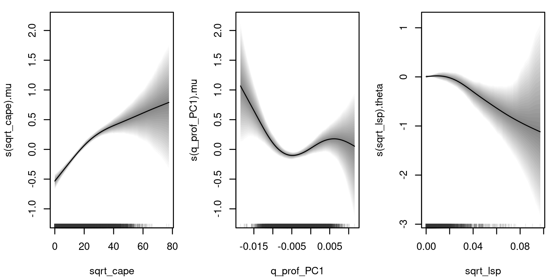
Refer to caption — Figure 9: Effect of the terms \codes(sqrt_cape) and \codes(q_prof_PC1) from the model \codemu and term \codes(sqrt_lsp) from model \codetheta. Credible intervals derived from MCMC samples.

\code

s(sqrt_cape) reveals a monotonic increasing shape. In the range from $0$ – $30$ the effect increases linearly with small credible intervals. For higher values the effect flattens and shows large credible intervals which are associated with the small amount of data in that range. Physically the shape of the effect is meaningful as more convective available potential energy has the potential to lead to heavier lightning events. \codes(q_prof_PC1) reveals areas of large credible intervals at the left and right bounds of the range due to small amount of data. In the mid-range an increasing effect is identified. As \codeq_prof_PC1 is the leading principal component of the vertical profile of specific humidity, one has to consider the corresponding spatial mode (not shown) for interpretation: Higher values of \codeq_prof_PC1 are linked to more moisture in the lower atmosphere, which is also available as a source of latent energy, i.e., energy that becomes free when water transfers from the gas to the liquid phase.

Finally it is interesting to look at the effect acting on the link scale of the parameter $\theta$ , \codes(sqrt_lsp) (right panel in Figure 9). \codesqrt_lsp is the square root of large scale precipitation, i.e., precipitation that is not linked to convective processes and thus it is not related to strong lightning events. The effect shows following relationship: Higher values of \codesqrt_lsp lead to smaller $\theta$ , which increases the variance of the distribution.

Before applying the model, i.e., predicting lightning cases before 2010, we check the marginal calibration of the distribution by hanging rootogram, a tool popular for the evaluation of count data regression models (Kleiber and Zeileis 2016). First we predict the distributional parameter on out-of-sample data \codeFlashAustriaEval for which lightning observations are on hand {Schunk} {Sinput} R> fit <- predict(b, newdata = FlashAustriaEval, type = "parameter") R> str(fit) {Soutput} List of 2 $mu:num[1:6000]0.01590.03280.01260.02650.0458...$ theta: num [1:6000] 0.000706 0.000707 0.000712 0.000709 0.000704 … \codepredict() returns a \codelist, of which each element is named as a distributional parameter and contains by default a vector of predictions. Each prediction is the average of the predictions obtained by all MCMC samples. The resulting \codelist can be used to derive further quantities by employing the functions of the \pkgbamlss family that can be extracted using \codefamily(), {Schunk} {Sinput} R> fam <- family(b) R> fam {Soutput} Family: ztnbinom Link function: mu = log, theta = log — Derivative functions: .. $score....$ mu .. .. $theta..$ hess .. .. $mu....$ theta The family contains functions to map the predictors to the parameter scale, density, cumulative distribution function, log-likelihood, and scores and Hessian. We apply the density to compute the expected frequencies of the positive counts. The function \code… ${d()}takesthequantileasfirstargument,andthe\code{list}withtheparameters,asreturnedby\code{predict()},asasecondargument.Theexpectedfrequenciescanthenbecomputedby\Schunk\Sinput R>expect<-sapply(1:50,function(j)sum(fam$d(j,fit)))Inordertoplottherootogram,wehavetonamethevectorandcoerceittoanobjectofclass\code{table}.Theverifyingobservedfrequenciescanbedirectlyobtainedby\code{table}.\Schunk\Sinput R>names(expect)<-1:50R>expect<-as.table(expect)R>obsrvd<-table(FlashAustriaEval$counts)[1:50]\par\begin{figure}\centering\includegraphics[]{bamlss-064} \@@toccaption{{\lx@tag[ ]{{10}}{Hanging rootogram for evaluating calibration of count data model on out-of-sample data. Red line indicates the expected frequencies on the square root scale. Gray bars indicate observed frequencies on square root scale hanging from the red line.}}}\@@caption{{\lx@tag[: ]{{Figure 10}}{Hanging rootogram for evaluating calibration of count data model on out-of-sample data. Red line indicates the expected frequencies on the square root scale. Gray bars indicate observed frequencies on square root scale hanging from the red line.}}} \@add@centering\end{figure}\par\begin{figure}\centering\includegraphics[]{bamlss-065} \@@toccaption{{\lx@tag[ ]{{11}}{ A probabilistic reconstruction of lightning counts occured on September 15 2001 at 6~UTC, 17~UTC and 23~UTC and on September 16 2001 at 13~UTC, i.e., the probability of having observed $10$ or more counts within one grid box.}}}\@@caption{{\lx@tag[: ]{{Figure 11}}{ A probabilistic reconstruction of lightning counts occured on September 15 2001 at 6~UTC, 17~UTC and 23~UTC and on September 16 2001 at 13~UTC, i.e., the probability of having observed $10$ or more counts within one grid box.}}}\@add@centering\end{figure}\par Theobservedandexpectedfrequenciescanbepluggedintothedefaultmethodof\code{rootogram}fromthe\pkg{countreg}package\cite[citep]{(\@@bibref{AuthorsPhrase1Year}{zeileis2008regression}{\@@citephrase{, }}{})}.\Schunk\Sinput R>library("countreg")R>rootogram(obsrvd,expect,xlab="#LightningCounts",main="Rootogram")Therootogramrevealsreasonablecalibrationofthemodelthoughitisslightlyunderestimatingthenumberofeventswithasinglelightningdischarge.NowgivengoodconvergenceandsamplecharacteristicsofthegradientboostingoptimizerandMCMCsampler,physicallyinterpretableeffects,andgoodout-of-samplecalibration,wecantakeourmodelandpredictacasefortheperiodbefore2010,forwhichnolightningdataareavailable.ThecaseofinterestisafrontmovingfromtheWesttotheEastontheNorthernsideoftheAlpson2001-09-15and2001-09-16.Thecasedata\code{FlashAustriaCase}containsadditionalcolumnscontainingtimeandspaceinformation,andisofclass\code{sf}\cite[citep]{(\@@bibref{AuthorsPhrase1Year}{pebesma2018sf}{\@@citephrase{, }}{})}.Wepredicttheparametersforthiscase,andderivetheprobabilityofobserving10ormoreflasheswithinagridboxconditionedonathunderstormactivity,byapplyingthecumulativedistributionfunction\code{...$p}ofthefamily\Schunk\Sinput R>library("sf")R>fit<-predict(b,newdata=FlashAustriaCase,type="parameter")R>FlashAustriaCase$P10<-1-fam$p(9,fit)Wevisualizethiscasebyemploying\code{ggplot()}\cite[citep]{(\@@bibref{AuthorsPhrase1Year}{wickham2016gg}{\@@citephrase{, }}{})},andtheOslocolorscalefromthe\pkg{colorspace}package\cite[citep]{(\@@bibref{AuthorsPhrase1Year}{zeileis2019colorspace}{\@@citephrase{, }}{})}.Thecountryborders\code{world}areretrievedfromthe\pkg{rnaturalearth}package\cite[citep]{(\@@bibref{AuthorsPhrase1Year}{south2017rnaturalearth}{\@@citephrase{, }}{})}.\Schunk\Sinput R>library("ggplot2")R>world<-rnaturalearth::ne_{c}ountries(scale="medium",returnclass="sf")R>ggplot()+geom_{s}f(aes(fill=P10),data=FlashAustriaCase)++scale_{f}ill_{c}ontinuous_{s}equential("Oslo",rev=TRUE)++geom_{s}f(data=world,col="white",fill=NA)++coord_{s}f(xlim=c(7.95,17),ylim=c(45.45,50),expand=FALSE)++facet_{w}rap(~time)+theme_{m}inimal()ThemapsareshowninFigure~\ref{fig:appcase}andrevealthattheprobabilityforstronglightningeventsincreasesduring2001-09-15between6and17~UTC.Duringnighttimethefrontoccurs,whichcanbenicelyseenat23~UTC.ThepropagationofthefrontisblockedbythemainAlpineridgelocatedat$ 47^∘ N $.Onthesubsequentday2001-09-16onecanseethattheprobabilityonthedownwindsideoftheAlpshasincreased.\par\par$

Acknowledgments

Thorsten Simon acknowledges the funding by the Austrian Science Fund (FWF, grant no. P31836)

References

Bivand et al. (2015) Bivand RS, Gómez-Rubio V, Rue H (2015). “Spatial Data Analysis with \proglangR-\pkgINLA with Some Extensions.” Journal of Statistical Software, 63(20), 1–31. 10.18637/jss.v063.i20.
Brezger et al. (2005) Brezger A, Kneib T, Lang S (2005). “\pkgBayesX: Analyzing Bayesian Structured Additive Regression Models.” Journal of Statistical Software, 14(11), 1–22. 10.18637/jss.v014.i11.
Brooks and Gelman (1998) Brooks SP, Gelman A (1998). “General Methods for Monitoring Convergence of Iterative Simulations.” Journal of Computational and Graphical Statistics, 7(4), 434–455. 10.1080/10618600.1998.10474787.
Bürkner (2017) Bürkner PC (2017). “\pkgbrms: An \proglangR Package for Bayesian Multilevel Models Using \pkgStan.” Journal of Statistical Software, 80(1), 1–28. 10.18637/jss.v080.i01.
Cameron and Trivedi (2013) Cameron AC, Trivedi PK (2013). Regression Analysis of Count Data. Econometric Society Monographs, 2nd edition. Cambridge University Press, Cambridge.
Carpenter et al. (2017) Carpenter B, Gelman A, Hoffman MD, Lee D, Goodrich B, Betancourt M, Brubaker M, Guo J, Li P, Riddell A (2017). “\proglangStan: A Probabilistic Programming Language.” Journal of Statistical Software, 76(1), 1–32. 10.18637/jss.v076.i01.
Chambers and Hastie (1992) Chambers JM, Hastie TJ (eds.) (1992). Statistical Models in \proglangS. Chapman & Hall, London.
Copernicus Climate Change Service (2017) Copernicus Climate Change Service (2017). “ERA5: Fifth Generation of ECMWF Atmospheric Reanalyses of the Global Climate.” Copernicus Climate Change Service Climate Date Store (CDS). Date of access: June 2019, https://cds.climate.copernicus.eu/cdsapp#!/home.
Dunn and Smyth (1996) Dunn PK, Smyth GK (1996). “Randomized Quantile Residuals.” Journal of Computational and Graphical Statistics, 5(3), 236–244. 10.2307/1390802.
Eilers and Marx (1996) Eilers PHC, Marx BD (1996). “Flexible Smoothing Using B-Splines and Penalized Likelihood.” Statistical Science, 11, 89–121. 10.1214/ss/1038425655.
Fahrmeir et al. (2004) Fahrmeir L, Kneib T, Lang S (2004). “Penalized Structured Additive Regression for Space Time Data: A Bayesian Perspective.” Statistica Sinica, 14, 731–761. 10.1007/978-3-642-34333-9_9.
Fahrmeir et al. (2013) Fahrmeir L, Kneib T, Lang S, Marx B (2013). Regression – Models, Methods and Applications. Springer-Verlag, Berlin.
Friedman et al. (2010) Friedman J, Hastie T, Tibshirani R (2010). “Regularization Paths for Generalized Linear Models via Coordinate Descent.” Journal of Statistical Software, 33(1), 1–22. 10.18637/jss.v033.i01.
Gamerman (1997) Gamerman D (1997). “Sampling from the Posterior Distribution in Generalized Linear Mixed Models.” Statistics and Computing, 7(1), 57–68. 10.1023/a:1018509429360.
Gelman (2006) Gelman A (2006). “Prior Distributions for Variance Parameters in Hierarchical Models (Comment on Article by Browne and Draper).” Bayesian Analysis, 1(3), 515–534. 10.1214/06-ba117a.
Gelman and Rubin (1992) Gelman A, Rubin DB (1992). “Inference from Iterative Simulation Using Multiple Sequences.” Statistical Science, 7(4), 457–472. 10.1214/ss/1177011136.
Gerfin (1996) Gerfin M (1996). “Parametric and Semi-Parametric Estimation of the Binary Response Model of Labour Market Participation.” Journal of Applied Econometrics, 11(3), 321–339. 10.1002/(SICI)1099-1255(199605)11:3<321::AID-JAE391>3.0.CO;2-K.
Gneiting et al. (2007) Gneiting T, Balabdaoui F, Raftery AE (2007). “Probabilistic Forecasts, Calibration and Sharpness.” Journal of the Royal Statistical Society B, 69(2), 243–268. 10.1111/j.1467-9868.2007.00587.x.
Gneiting and Raftery (2007) Gneiting T, Raftery AE (2007). “Strictly Proper Scoring Rules, Prediction, and Estimation.” Journal of the American Statistical Association, 102(477), 359–378. 10.1198/016214506000001437.
Groll et al. (2019) Groll A, Hambuckers J, Kneib T, Umlauf N (2019). “LASSO-Type Penalization in the Framework of Generalized Additive Models for Location, Scale and Shape.” Computational Statistics & Data Analysis, 140, 59–74. 10.1016/j.csda.2019.06.005.
Hastie and Tibshirani (1990) Hastie T, Tibshirani R (1990). Generalized Additive Models. Chapman & Hall/CRC, New York.
Heidelberger and Welch (1981) Heidelberger P, Welch PD (1981). “A Spectral Method for Confidence Interval Generation and Run Length Control in Simulations.” Communications of the ACM, 24(4), 233–245. 10.1145/358598.358630.
Heidelberger and Welch (1983) Heidelberger P, Welch PD (1983). “Simulation Run Length Control in the Presence of an Initial Transient.” Operations Research, 31(6), 1109–1144. 10.1287/opre.31.6.1109.
Herwartz et al. (2016) Herwartz H, Klein N, Strumann C (2016). “Modelling Hospital Admission and Length of Stay by Means of Generalised Count Data Models.” Journal of Applied Econometrics, 31(6), 1159–1182. 10.1002/jae.2454.
Hofner et al. (2016) Hofner B, Mayr A, Schmid M (2016). “\pkggamboostLSS: An \proglangR Package for Model Building and Variable Selection in the GAMLSS Framework.” Journal of Statistical Software, 74(1), 1–31. 10.18637/jss.v074.i01.
Jordan et al. (2019) Jordan A, Krüger F, Lerch S (2019). “Evaluating Probabilistic Forecasts with \pkgscoringRules.” Journal of Statistical Software, 90(12), 1–37. 10.18637/jss.v090.i12.
Kleiber and Zeileis (2008) Kleiber C, Zeileis A (2008). Applied Econometrics with \proglangR. Springer-Verlag, New York. URL https://CRAN.R-project.org/package=AER.
Kleiber and Zeileis (2016) Kleiber C, Zeileis A (2016). “Visualizing Count Data Regressions Using Rootograms.” The American Statistician, 70(3), 296–303. 10.1080/00031305.2016.1173590.
Klein et al. (2014) Klein N, Denuit M, Lang S, Kneib T (2014). “Nonlife Ratemaking and Risk Management with Bayesian Generalized Additive Models for Location, Scale, and Shape.” Insurance: Mathematics and Economics, 55, 225 – 249. 10.1016/j.insmatheco.2014.02.001.
Klein and Kneib (2016a) Klein N, Kneib T (2016a). “Scale-Dependent Priors for Variance Parameters in Structured Additive Distributional Regression.” Bayesian Analysis, 11(4), 1071–1106. 10.1214/15-ba983.
Klein and Kneib (2016b) Klein N, Kneib T (2016b). “Simultaneous Inference in Structured Additive Conditional Copula Regression Models: A Unifying Bayesian Approach.” Statistics and Computing, 26(4), 841–860. 10.1007/s11222-015-9573-6.
Klein et al. (2015a) Klein N, Kneib T, Klasen S, Lang S (2015a). “Bayesian Structured Additive Distributional Regression for Multivariate Responses.” Journal of the Royal Statistical Society C, 64, 569–591. 10.1111/rssc.12090.
Klein et al. (2015b) Klein N, Kneib T, Lang S (2015b). “Bayesian Generalized Additive Models for Location, Scale and Shape for Zero-Inflated and Overdispersed Count Data.” Journal of the American Statistical Association, 110(509), 405–419. 10.1080/01621459.2014.912955.
Klein et al. (2015c) Klein N, Kneib T, Lang S, Sohn A (2015c). “Bayesian Structured Additive Distributional Regression with an Application to Regional Income Inequality in Germany.” Annals of Applied Statistics, 9, 1024–1052. 10.1214/15-aoas823.
Klein et al. (2019) Klein N, Simon T, Umlauf N (2019). “Neural Network Regression with an Application to Leukaemia Survival Data – An Unstructured Distributional Approach.” In Proceedings of the 34th International Workshop on Statistical Modelling, Guimarães, Portugal, volume 1, pp. 157–160. Statistical Modelling Society.
Köhler et al. (2017) Köhler M, Umlauf N, Beyerlein A, Winkler C, Ziegler AG, Greven S (2017). “Flexible Bayesian Additive Joint Models with an Application to Type 1 Diabetes Research.” Biometrical Journal, 59(6), 1144–1165. 10.1002/bimj.201600224.
Köhler et al. (2018) Köhler M, Umlauf N, Greven S (2018). “Nonlinear Association Structures in Flexible Bayesian Additive Joint Models.” Statistics in Medicine, 37(30), 4771–4788. 10.1002/sim.7967.
Lindgren and Rue (2015) Lindgren F, Rue H (2015). “Bayesian Spatial Modelling with \proglangR-\pkgINLA.” Journal of Statistical Software, 63(19), 1–25. 10.18637/jss.v063.i19.
Lunn et al. (2000) Lunn DJ, Thomas A, Best N, Spiegelhalter D (2000). “\pkgWinBUGS – A Bayesian Modelling Framework: Concepts, Structure, and Extensibility.” Statistics and Computing, 10, 325–337. 10.1023/a:1008929526011.
Mayr et al. (2012) Mayr A, Fenske N, Hofner B, Kneib T, Schmid M (2012). “Generalized Additive Models for Location, Scale and Shape for High Dimensional Data: A Flexible Approach Based on Boosting.” Journal of the Royal Statistical Society C, 61(3), 403–427. 10.1111/j.1467-9876.2011.01033.x.
Neal (2003) Neal RM (2003). “Slice Sampling.” The Annals of Statistics, 31(3), 705–767. 10.1214/aos/1056562461.
Nelder and Wedderburn (1972) Nelder JA, Wedderburn RWM (1972). “Generalized Linear Models.” Journal of the Royal Statistical Society A, 135, 370–384. 10.2307/2344614.
Pebesma (2018) Pebesma E (2018). “Simple Features for \proglangR: Standardized Support for Spatial Vector Data.” The \proglangR Journal, 10(1), 439–446. 10.32614/RJ-2018-009.
Plummer (2003) Plummer M (2003). “\pkgJAGS: A Program for Analysis of Bayesian Graphical Models Using Gibbs Sampling.” In K Hornik, F Leisch, A Zeileis (eds.), Proceedings of the 3rd International Workshop on Distributed Statistical Computing, Vienna, Austria. URL http://www.ci.tuwien.ac.at/Conferences/DSC-2003/Proceedings/.
Plummer et al. (2006) Plummer M, Best N, Cowles K, Vines K (2006). “\pkgcoda: Convergence Diagnosis and Output Analysis for MCMC.” \proglangR News, 6(1), 7–11.
Polson and Scott (2012) Polson NG, Scott JG (2012). “On the Half-Cauchy Prior for a Global Scale Parameter.” Bayesian Analysis, 7(4), 887–902. 10.1214/12-ba730.
\proglangR Core Team (2019) \proglangR Core Team (2019). \proglangR: A Language and Environment for Statistical Computing. \proglangR Foundation for Statistical Computing, Vienna, Austria. URL https://www.R-project.org/.
Rigby and Stasinopoulos (2005) Rigby RA, Stasinopoulos DM (2005). “Generalized Additive Models for Location, Scale and Shape.” Journal of the Royal Statistical Society C, 54(3), 507–554. 10.1111/j.1467-9876.2005.00510.x.
Rue et al. (2009) Rue H, Martino S, Chopin N (2009). “Approximate Bayesian Inference for Latent Gaussian Models by Using Integrated Nested Laplace Approximations.” Journal of the Royal Statistical Society B, 71(2), 319–392. 10.1111/j.1467-9868.2008.00700.x.
Schulz et al. (2005) Schulz W, Cummins K, Diendorfer G, Dorninger M (2005). “Cloud-to-Ground Lightning in Austria: A 10-Year Study Using Data from a Lightning Location System.” Journal of Geophysical Research: Atmospheres, 110(D9). 10.1029/2004JD005332.
Silverman (1985) Silverman BW (1985). “Some Aspects of the Spline Smoothing Approach to Non-Parametric Regression Curve Fitting.” Journal of the Royal Statistical Society B, 47(1), 1–21. 10.1111/j.2517-6161.1985.tb01327.x.
Simon (2019) Simon T (2019). \pkgFlashAustria: Data and Model for Reanalyzing Flash Counts in Austria. \proglangR package version 0.1-0/r3479, URL https://R-Forge.R-project.org/projects/bayesr/.
Simon et al. (2018) Simon T, Fabsic P, Mayr GJ, Umlauf N, Zeileis A (2018). “Probabilistic Forecasting of Thunderstorms in the Eastern Alps.” Monthly Weather Review, 146, 2999–3009. 10.1175/MWR-D-17-0366.1.
Simon et al. (2019) Simon T, Mayr GJ, Umlauf N, Zeileis A (2019). “NWP-Based Lightning Prediction Using Flexible Count Data Regression.” Advances in Statistical Climatology, Meteorology and Oceanography, 5(1), 1–16. 10.5194/ascmo-5-1-2019.
Smyth (1996) Smyth GK (1996). “Partitioned Algorithms for Maximum Likelihood and Other Non-Linear Estimation.” Statistics and Computing, 6(3), 201–216. 10.1007/bf00140865.
South (2017) South A (2017). \pkgrnaturalearth: World Map Data from Natural Earth. \proglangR package version 0.1.0, URL https://CRAN.R-project.org/package=rnaturalearth.
Spiegelhalter et al. (2002) Spiegelhalter DJ, Best NG, Carlin BP, Van der Linde A (2002). “Bayesian Measures of Model Complexity and Fit.” Journal of the Royal Statistical Society B, 64(4), 583–639. 10.1111/1467-9868.00353.
Stadlmann (2019) Stadlmann S (2019). \pkgdistreg.vis: Framework for the Visualization of Distributional Regression Models. \proglangR package version 1.5.0, URL https://CRAN.R-project.org/package=distreg.vis.
Stasinopoulos and Rigby (2007) Stasinopoulos DM, Rigby RA (2007). “Generalized Additive Models for Location Scale and Shape (GAMLSS) in \proglangR.” Journal of Statistical Software, 23(7), 1–46. 10.18637/jss.v023.i07.
Stasinopoulos and Rigby (2019a) Stasinopoulos DM, Rigby RA (2019a). \pkggamlss: Generalised Additive Models for Location, Scale and Shape. \proglangR package version 5.1-3, URL https://CRAN.R-project.org/package=gamlss.
Stasinopoulos and Rigby (2019b) Stasinopoulos DM, Rigby RA (2019b). \pkggamlss.dist: Distributions for Generalized Additive Models for Location, Scale and Shape. \proglangR package version 5.1-4, URL https://CRAN.R-project.org/package=gamlss.dist.
Umlauf et al. (2015) Umlauf N, Adler D, Kneib T, Lang S, Zeileis A (2015). “Structured Additive Regression Models: An \proglangR Interface to \pkgBayesX.” Journal of Statistical Software, 63(21), 1–46. 10.18637/jss.v063.i21.
Umlauf et al. (2018) Umlauf N, Klein N, Zeileis A (2018). “BAMLSS: Bayesian Additive Models for Location, Scale, and Shape (and Beyond).” Journal of Computational and Graphical Statistics, 27(3), 612–627. 10.1080/10618600.2017.1407325.
Umlauf and Kneib (2018) Umlauf N, Kneib T (2018). “A Primer on Bayesian Distributional Regression.” Statistical Modelling, 18(3-4), 219–247. 10.1177/1471082X18759140.
Van Buuren and Fredriks (2001) Van Buuren S, Fredriks M (2001). “Worm Plot: A Simple Diagnostic Device for Modelling Growth Reference Curves.” Statistics in Medicine, 20(8), 1259–1277. 10.1002/sim.746.
Wasserstein and Lazar (2016) Wasserstein RL, Lazar NA (2016). “The ASA Statement on $p$ -Values: Context, Process, and Purpose.” The American Statistician, 70(2), 129–133. 10.1080/00031305.2016.1154108.
Watanabe (2010) Watanabe S (2010). “Asymptotic Equivalence of Bayes Cross Validation and Widely Applicable Information Criterion in Singular Learning Theory.” Journal of Machine Learning Research, 11, 3571–3594.
Wickham (2016) Wickham H (2016). \pkgggplot2: Elegant Graphics for Data Analysis. Springer-Verlag, New York.
Wood (2016) Wood SN (2016). “Just Another Gibbs Additive Modeler: Interfacing \pkgJAGS and \pkgmgcv.” Journal of Statistical Software, 75(7), 1–15. 10.18637/jss.v075.i07.
Wood (2017) Wood SN (2017). Generalized Additive Models: An Introduction with \proglangR. 2nd edition. Chapman & Hall/CRC, Boca Raton.
Wood (2019) Wood SN (2019). \pkgmgcv: Mixed GAM Computation Vehicle with Automatic Smoothness Estimation. \proglangR package version 1.8.28, URL https://CRAN.R-project.org/package=mgcv.
Wood et al. (2017) Wood SN, Li Z, Shaddick G, Augustin NH (2017). “Generalized Additive Models for Gigadata: Modelling the UK Black Smoke Network Daily Data.” Journal of the American Statistical Association, 112(519), 1199–1210. 10.1080/01621459.2016.1195744.
Wood et al. (2016) Wood SN, Pya N, Säfken B (2016). “Smoothing Parameter and Model Selection for General Smooth Models.” Journal of the American Statistical Association, 111(516), 1548–1563. 10.1080/01621459.2016.1180986.
Yee (2010) Yee TW (2010). “The \pkgVGAM Package for Categorical Data Analysis.” Journal of Statistical Software, 32(10), 1–34. 10.18637/jss.v032.i10.
Zeileis and Croissant (2010) Zeileis A, Croissant Y (2010). “Extended Model Formulas in \proglangR: Multiple Parts and Multiple Responses.” Journal of Statistical Software, 34(1), 1–13. 10.18637/jss.v034.i01.
Zeileis et al. (2019) Zeileis A, Fisher JC, Hornik K, Ihaka R, McWhite CD, Murrell P, Stauffer R, Wilke CO (2019). “\pkgcolorspace: A Toolbox for Manipulating and Assessing Colors and Palettes.” arXiv 1903.06490, arXiv.org E-Print Archive. URL http://arxiv.org/abs/1903.06490.
Zeileis et al. (2008) Zeileis A, Kleiber C, Jackman S (2008). “Regression Models for Count Data in \proglangR.” Journal of Statistical Software, 27(1), 1–25. 10.18637/jss.v027.i08.

Appendix A Custom CRPS() function

The \proglangR package \pkgscoringRules (Jordan et al. 2019) provides tools for model calibration checks. A commonly used measure is the CRPS. Since the number of candidate distributions in BAMLSS is quite large, it can happen that the CRPS for some distributions is not implemented. In such a case the reader can implement the CRPS using numerical integration. The following \proglangR code implements the CRPS() to be used with \pkgbamlss and a numeric response, e.g., which can be used with the motorcycle accident model presented in Section 2.3. {Schunk} {Sinput} R> CRPS <- function(object, newdata = NULL) + yname <- response_name(object) + fam <- family(object) + if(is.null(fam ${p))+stop("nop()functioninfamilyobject!")+if(is.null(newdata))+newdata<-model.frame(object)+n<-nrow(newdata)+crps<-rep(0,n)+par<-as.data.frame(predict(object,newdata=newdata,type="parameter"))+for(iin1:n){+foo<-function(y){+(fam$p(y,par[i,,drop=FALSE])-1*(y>=newdata[[yname]][i]))^{2}+}+crps[i]<-integrate(foo,-Inf,Inf)$value+}+return(crps)+}\par\par\par$

Appendix B Gaussian family object

The following \proglangR code shows an example implementation of the Gaussian distribution as presented in Section 4.2. {Schunk} {Sinput} R> Gauss_bamlss <- function(…) + f <- list( + "family" = "mygauss", + "names" = c("mu", "sigma"), + "links" = c(mu = "identity", sigma = "log"), + "d" = function(y, par, log = FALSE) + dnorm(y, mean = par $mu,sd=par$ sigma, log = log) + , + "p" = function(y, par, …) + pnorm(y, mean = par $mu,sd=par$ sigma, …) + , + "r" = function(n, par) + rnorm(n, mean = par $mu,sd=par$ sigma) + , + "q" = function(p, par) + qnorm(p, mean = par $mu,sd=par$ sigma) + , + "score" = list( + mu = function(y, par, …) + drop((y - par $mu)/(par$ sigma^2)) + , + sigma = function(y, par, …) + drop(-1 + (y - par $mu)^{2}/(par$ sigma^2)) + + ), + "hess" = list( + mu = function(y, par, …) + drop(1 / (par ${{sigma^{2}))+},+sigma=function(y,par,...){+rep(2,length(y))+}+)+)+class(f)<-"family.bamlss"+return(f)+}\par\par\par$

Appendix C Special model terms

The default estimation engines bfit() and GMCMC() (also the gradient boosting optimizer function boost()) in \pkgbamlss provide support for the implementation of special model terms, i.e., model terms that cannot be represented by the \pkgmgcv smooth term constructor infrastructures. One simple example of such a special model term is a nonlinear growth curve, e.g., a nonlinear Gompertz curve

f(x;\boldsymbol{\beta})=\beta_{1}\cdot\exp(-\beta_{2}\cdot\exp(-\beta_{3}\cdot x)),

but also the lasso model term constructor la() presented in Section 2.2 is a special \pkgbamlss model term. The special model term constructor is needed in this case, since the growth curve is nonlinear in the parameters $\boldsymbol{\beta}$ , hence, the default backfitting and sampling strategies cannot be applied. Fortunately, estimation algorithms in distributional regression can be split into separate updating equations (see also Section 3.2). This means that each model term can have its own updating function. The user interested in this feature only needs to write a new smooth.construct() and Predict.matrix() method.

The following \proglangR code implements a Gompertz growth model term which can be used by the default optimizer function bfit() and sampling function GMCMC() of the \pkgbamlss package. The new smooth.construct() method is {Schunk} {Sinput} R> smooth.construct.gc.smooth.spec <- function(object, data, knots) + + object $X<-matrix(as.numeric(data[[object$ term]]), ncol = 1) + center <- if(!is.null(object $xt$ center)) + object $xt$ center + else TRUE + object $by.done<-TRUE+if(object$ by != "NA") + stop("by variables not supported!") + + ## Begin special elements to be used with bfit() and GMCMC(). + object $fit.fun<-function(X,b,...){+f<-b[1]*exp(-b[2]*exp(-b[3]*drop(X)))+if(center)+f<-f-mean(f)+f+}+object$ update <- bfit_optim + object $propose<-GMCMC_{s}lice+object$ prior <- function(b) sum(dnorm(b, sd = 1000, log = TRUE)) + object $fixed<-TRUE+object$ state $parameters<-c("b1"=0,"b2"=0.5,"b3"=0.1)+object$ state $fitted.values<-rep(0,length(object$ X)) + object $state$ edf <- 3 + object ${special.npar<-3##Important!+##Endspecialelements.++##Important,Thisisaspecialsmoothconstructor!+class(object)<-c("gc.smooth","no.mgcv","special")++object+}Inprinciple,thesetupisverysimilartothesmoothconstructorfunctionsprovidedbythe\pkg{mgcv}package.Onlyfewelementsneedtobeadded:\begin{itemize}\itemize@item@{{fit.fun()}{\@index{\@indexphrase[fit.fun]{{fit.fun()}}}}}: A function of the data \code{X} and parameter vector \code{b} that evaluates the fitted values. \par\vskip 4.0pt\vskip 4.0pt plus 2.0pt minus 1.0pt\itemize@item@{{update()}{\@index{\@indexphrase[update]{{update()}}}}}: An updating function to be used with optimizer {{bfit()}{\@index{\@indexphrase[bfit]{{bfit()}}}}}. \par\vskip 4.0pt\vskip 4.0pt plus 2.0pt minus 1.0pt\itemize@item@{{propose()}{\@index{\@indexphrase[propose]{{propose()}}}}}: A MCMC propose function to be used with sampler {{GMCMC()}{\@index{\@indexphrase[GMCMC]{{GMCMC()}}}}}. \par\vskip 4.0pt\vskip 4.0pt plus 2.0pt minus 1.0pt\itemize@item@{{prior()}{\@index{\@indexphrase[prior]{{prior()}}}}}: Function of the parameters \code{b} that evaluates the log-prior. Note, additional functions can be {{grad()}{\@index{\@indexphrase[grad]{{grad()}}}}} and \code{hess} that evaluate the first and second derivative of the log-prior w.r.t.\ the parameters \code{b}. \par\vskip 4.0pt\vskip 4.0pt plus 2.0pt minus 1.0pt\itemize@item@\code{fixed}: Is the number of degrees of freedom fixed or not? \par\vskip 4.0pt\vskip 4.0pt plus 2.0pt minus 1.0pt\itemize@item@\code{state}: This is a named list with starting values for the \code{"parameters"}, the \code{"fitted.values"} and degrees of freedom \code{"edf"}. Note that regression coefficients are always named with \code{"b*"} and shrinkage or smoothing variances with \code{"tau2*"} in the \code{"parameters"} vector. \par\vskip 4.0pt\vskip 4.0pt plus 2.0pt minus 1.0pt\itemize@item@\code{special.npar}: How many parameters does this model term have in total? This is needed for internal setup, because the Gompertz function has three parameters but the design matrix only one column. \end{itemize}Tocomputepredictionsofthismodeltermanewmethodforthe{\texttt{Predict.matrix()}{\@index{\@indexphrase[Predict.matrix]{{Predict.matrix()}}}}}functionneedstobeimplemented,too.\Schunk\Sinput R>Predict.matrix.gc.smooth<-function(object,data,knots)+{+X<-matrix(as.numeric(data[[object$term]]),ncol=1)+X+}\par Specialmodeltermscanthenbeusedwiththeconstructorfunction{\texttt{s2()}{\@index{\@indexphrase[s2]{{s2()}}}}}.Toillustratethethisfeaturein\pkg{bamlss},wesimulateheteroskedasticgrowthdatawith$ $\texttt{y}\sim\mathcal{N}(\mu=2+1/(1+\exp(0.5\cdot(15-\texttt{time}))),\log(\sigma)=-3+2\cdot\cos(\texttt{time}/30\cdot 6-3))$ $andsubsequentlyestimatethemodelwithslicesampling\cite[citep]{(\@@bibref{AuthorsPhrase1Year}{bamlss:Neal:2003}{\@@citephrase{, }}{})}for$ β $intheMCMCalgorithmusingthefollowing\proglang{R}code\begin{figure}\centering\includegraphics[]{bamlss-074} \includegraphics[]{bamlss-075} \@@toccaption{{\lx@tag[ ]{{12}}{ Estimated nonlinear effects on parameter $\mu$ and $\sigma$ of the simulated growth curve example. Gray shaded areas represent 95\% credible intervals.}}}\@@caption{{\lx@tag[: ]{{Figure 12}}{ Estimated nonlinear effects on parameter $\mu$ and $\sigma$ of the simulated growth curve example. Gray shaded areas represent 95\% credible intervals.}}}\@add@centering\end{figure}\Schunk\Sinput R>set.seed(111)R>d<-data.frame("time"=1:30)R>d$y<-2+1/(1+exp(0.5*(15-d$time)))++rnorm(30,sd=exp(-3+2*cos(d$time/30*6-3)))R>f<-list(+y~s2(time,bs="gc"),+sigma~s(time)+)R>b<-bamlss(f,data=d,optimizer=bfit,sampler=GMCMC)R>plot(b)TheestimatedeffectsareshowninFigure~\ref{fig:gcurve}.Thegrowthcurvemeanfunctionestimateseemstofitthedataquitewell.Also,thenonlinearrelationshipforparameter$ σ $couldbecapturedbythemodel.\par Insummary,inordertobuildupspecial\pkg{bamlss}modeltermsonlyafewthingshavetobeconsidered.Theexample\proglang{R}codefortheGompertzsmoothconstructorgivenhereisagoodstartingpointforreadersinterestedinusingthisfeature.\par\par\par$

Appendix D Model fitting engines for linear regression

In the following, to explain the setup and the naming convention of estimation engines in more detail, we implement

•

a new family object for simple linear models $y=x^{\top}\boldsymbol{\beta}+\varepsilon$ with $\varepsilon\sim N(0,\sigma^{2})$ ,
•

and set up an optimizer function,
•

and additionally a MCMC sampling function.

For illustration, the family object is kept very simple, we only model the mean function in terms of covariates. {Schunk} {Sinput} R> lm_bamlss <- function(…) + f <- list( + "family" = "LM", + "names" = "mu", + "links" = "identity", + "d" = function(y, par, log = FALSE) + sigma <- sqrt(sum((y - par $mu)^{2})/(length(y)-.lm_{b}amlss.p))+dnorm(y,mean=par$ mu, sd = sigma, log = log) + , + "p" = function(y, par, …) + sigma <- sqrt(sum((y - par $mu)^{2})/(length(y)-.lm_{b}amlss.p))+pnorm(y,mean=par$ mu, sd = sigma, …) + + ) + class(f) <- "family.bamlss" + return(f) + Now, for setting up the estimation functions we first simulate some data using the GAMart() function, afterwards the necessary \code"bamlss.frame" can be created with {Schunk} {Sinput} R> d <- GAMart() R> bf <- bamlss.frame(num x1 + x2, data = d, family = "lm") R> print(bf) {Soutput} ’bamlss.frame’ structure: .. $call..$ model.frame .. $formula..$ family .. $terms..$ x .. .. $mu......$ formula .. .. .. $fake.formula......$ terms .. .. .. $model.matrix..$ y .. .. $numAsnotedabove,theobjectisanamedlistwithelements\code{"x"}and\code{"y"},whichwillbepassedtotheestimationfunctions.Forthemoment,sinceweonlyimplementalinearmodel,weneedtoworkwiththelinearmodelmatrixthatispartofthe\code{bf}object.\Schunk\Sinput R>head(bf$x$mu$model.matrix)\Soutput(Intercept)x1x2110.29051020.32659717210.50900360.03047384310.39004980.82453055410.36504580.24858952510.52199090.19089833610.19779140.65983122andtheresponse\code{y}\Schunk\Sinput R>head(bf$y)\Soutput num10.223272520.247957630.12215804-0.13708225-0.11089886-0.1011208tosetuptheoptimizerfunctionwith:\Schunk\Sinput R>lm.opt<-function(x,y,...)+{+##Onlyunivariateresponse.+y<-y[[1L]]++##Forillustrationthisiseasiertoread.+X<-x$mu$model.matrix++##Estimatemodelparameters.+par<-drop(chol2inv(chol(crossprod(X)))++##Setparameternames.+names(par)<-paste0("mu.p.",colnames(X))++##Returnestimatedparametersandfittedvalues.+rval<-list(+"parameters"=par,+"fitted.values"=drop(X+"edf"=length(par),+"sigma"=drop(sqrt(crossprod(y-X+)++##Setedfwithin.GlobalEnvforthe+##loglik()functioninthelm_{b}amlss()family.+.lm_{b}amlss.p<<-length(par)++return(rval)+}Thisoptimizerfunctioncanalreadybeusedwiththe{\texttt{bamlss()}{\@index{\@indexphrase[bamlss]{{bamlss()}}}}}wrapperfunctionandallextractorfunctionsarereadilyavailable.\Schunk\Sinput R>f<-num~x1+poly(x2,5)+poly(x3,5)R>b<-bamlss(f,data=d,family="lm",optimizer=lm.opt,sampler=FALSE)R>summary(b)\Soutput Call:bamlss(formula=f,family="lm",data=d,optimizer=lm.opt,sampler=FALSE)---Family:LMLinkfunction:mu=identity*---Formulamu:---num~x1+poly(x2,5)+poly(x3,5)-Parametriccoefficients:parameters(Intercept)0.199x1-0.653poly(x2,5)1-1.791poly(x2,5)22.014poly(x2,5)30.474poly(x2,5)4-1.752poly(x2,5)50.743poly(x3,5)1-0.303poly(x3,5)24.273poly(x3,5)30.050poly(x3,5)40.572poly(x3,5)50.144---Optimizersummary:-edf=12sigma=0.2257---\Sinput R>nd<-data.frame("x2"=seq(0,1,length=100))R>nd$p<-predict(b,newdata=nd,term="x2")Plottheestimatedeffectofvariable\code{x2}.\Schunk\Sinput R>plot2d(p~x2,data=nd)\par ThenextstepistosetupafullBayesianMCMCsamplingfunction.Fortunately,ifweassumemultivariatenormalpriorsfortheregressioncoefficientsandaninverseGammapriorforthevariance,aGibbssamplerwithmultivariatenormalandinverseGammafullconditionalscanbecreated.TheMCMCalgorithmconsecutivelysamplesfor$ t = 1, …, T $fromthefullconditionals$ $\boldsymbol{\beta}^{(t)}|\cdot\sim N\left(\boldsymbol{\mu}_{\boldsymbol{\beta}}^{(t-1)},\boldsymbol{\Sigma}_{\boldsymbol{\beta}}^{(t-1)}\right)$ $and$ ${\sigma^{2}}^{(t)}|\cdot\sim IG\left({a^{\prime}}^{(t-1)},{b^{\prime}}^{(t-1)}\right),$ $where$ IG( ⋅) $istheinverseGammadistributionforsamplingthevarianceparameter.Thecovariancematrixfor$ β $isgivenby$ $\boldsymbol{\Sigma}_{\boldsymbol{\beta}}=\left(\frac{1}{\sigma^{2}}\mathbf{X}^{\top}\mathbf{X}+\frac{1}{\sigma^{2}}\mathbf{M}^{-1}\right)^{-1}$ $andthemean$ $\boldsymbol{\mu}_{\boldsymbol{\beta}}=\boldsymbol{\Sigma}_{\boldsymbol{\beta}}\left(\frac{1}{\sigma^{2}}\mathbf{X}^{\top}\mathbf{y}+\frac{1}{\sigma^{2}}\mathbf{M}^{-1}\mathbf{m}\right),$ $where$ m $isthepriormeanand$ M $thepriorcovariancematrix.Similarly,for$ σ^2 $paramaters$ a^′ $and$ b^′ $arecomputedby$ $a^{\prime}=a+\frac{n}{2}+\frac{p}{2}$ $and$ $b^{\prime}=b+\frac{1}{2}(\mathbf{y}-\mathbf{X}\boldsymbol{\beta})^{\top}(\mathbf{y}-\mathbf{X}\boldsymbol{\beta})+\frac{1}{2}(\boldsymbol{\beta}-\mathbf{m})^{\top}\mathbf{M}^{-1}(\boldsymbol{\beta}-\mathbf{m}),$ $where$ a $and$ b $areusuallysetsmall,e.g.,with$ a = 1 $and$ b = 0.0001 ${,suchthatthepriorisflatanduninformative.\par WecanimplementtheMCMCalgorithminthefollowingsamplingfunction\Schunk\Sinput R>lm.mcmc<-function(x,y,start=NULL,+n.iter=12000,burnin=2000,thin=10,+m=0,M=1e+05,+a=1,b=1e-05,+verbose=TRUE,...)+{+##Howmanysamplesaresaved?+itrthin<-seq.int(burnin,n.iter,by=thin)+nsaves<-length(itrthin)++##Onlyunivariateresponse.+y<-y[[1L]]++##Forillustrationthisiseasiertoread.+X<-x$mu$model.matrix++##Again,setedfwithin.GlobalEnvforthe+##loglik()functioninthelm_{b}amlss()family.+.lm_{b}amlss.p<<-ncol(X)++##Numberofobservationsandparameters.+n<-length(y)+p<-ncol(X)++##Matrixsavingthesamples.+samples<-matrix(0,nsaves,p+1L)++##Sticktothenamingconvention.+pn<-paste0("mu.p.",colnames(X))+colnames(samples)<-c(+pn,##Regressioncoefficientsand+"sigma"##variancesamples.+)++##Setupcoefficientvector,+##again,usecorrectnames.+beta<-rep(0,p)+names(beta)<-pn+sigma<-sd(y)++##Checkforstartingvaluesobtained,+##e.g.,fromlm.opt()fromabove.+if(!is.null(start)){+sn<-names(start)+for(jinnames(beta)){+if(j+beta[j]<-start[j]+}+}++##Processpriorinformation.+m<-rep(m,length.out=p)+if(length(M)<2)+M<-rep(M,length.out=p)+if(!is.matrix(M))+M<-diag(M)+Mi<-solve(M)++##Precomputecrossproducts.+XX<-crossprod(X)+Xy<-crossprod(X,y)++##Inversegammaparameter.+a<-a+n/2+p/2++##Startsampling.+ii<-1+for(iin1:n.iter){+##Samplingsigma+b2<-b+1/2*t(y-X+1/2*t(beta-m)+sigma2<-sqrt(1/rgamma(1,a,b2))++##Samplingbeta.+sigma2i<-1/sigma2+Sigma<-chol2inv(chol(sigma2i*XX+sigma2i*Mi))+mu<-Sigma+beta<-MASS::mvrnorm(1,mu,Sigma)++if(i+samples[ii,pn]<-beta+samples[ii,"sigma"]<-sqrt(sigma2)+ii<-ii+1+}+if(verbose){+if(i+cat("iteration:",i,"\n")+}+}++##Convertto"mcmc"object.+samples<-as.mcmc(samples)++return(samples)+}Thenewsamplingfunctioncanbedirectlyusedwiththe{\texttt{bamlss()}{\@index{\@indexphrase[bamlss]{{bamlss()}}}}}wrapper\Schunk\Sinput R>b<-bamlss(f,data=d,family="lm",optimizer=lm.opt,sampler=lm.mcmc)\Soutput iteration:1000iteration:2000iteration:3000iteration:4000iteration:5000iteration:6000iteration:7000iteration:8000iteration:9000iteration:10000iteration:11000iteration:12000\Sinput R>summary(b)\Soutput Call:bamlss(formula=f,family="lm",data=d,optimizer=lm.opt,sampler=lm.mcmc)---Family:LMLinkfunction:mu=identity*---Formulamu:---num~x1+poly(x2,5)+poly(x3,5)-Parametriccoefficients:Mean2.5(Intercept)0.199370.114430.197990.284020.199x1-0.65380-0.79612-0.65227-0.51375-0.653poly(x2,5)1-1.79249-2.71924-1.79813-0.86320-1.791poly(x2,5)22.000101.080571.990222.883332.014poly(x2,5)30.48731-0.487800.494881.494460.474poly(x2,5)4-1.78055-2.66888-1.78927-0.81921-1.752poly(x2,5)50.73783-0.280790.742571.722150.743poly(x3,5)1-0.29363-1.25928-0.293050.56080-0.303poly(x3,5)24.290663.364964.281255.269034.273poly(x3,5)30.03256-0.985500.058191.016700.050poly(x3,5)40.57143-0.365140.585631.489130.572poly(x3,5)50.13204-0.810590.134341.074700.144---Samplersummary:-DIC=23.3951pd=52.4174runtime=2.483---Optimizersummary:-edf=12sigma=0.2257---\Sinput R>##Predictforalltermsincluding95R>nd$x1<-nd$x3<-seq(0,1,length=100)R>for(jinc("x1","x2","x3")){+nd[[paste0("p.",j)]]<-predict(b,newdata=nd,term=j,+FUN=c95,intercept=FALSE)+}Theestimatedeffectscanbeplottedwith:\Schunk\Sinput R>par(mfrow=c(1,3))R>plot2d(p.x1~x1,data=nd,fill.select=c(0,1,0,1),lty=c(2,1,2))R>plot2d(p.x2~x2,data=nd,fill.select=c(0,1,0,1),lty=c(2,1,2))R>plot2d(p.x3~x3,data=nd,fill.select=c(0,1,0,1),lty=c(2,1,2))\par\par\lx@frontmatter@fallback\@add@PDF@RDFa@triples\par\end{document}$