A Phase Shift Deep Neural Network for High Frequency Approximation and Wave Problems Thanks: to be submitted to SISC.

Wei Cai Thanks: Department of Mathematics, Southern Methodist University, Dallas, TX 75275, USA. Xiaoguang Li Thanks: MOE-LCSM, School of Mathematics and Statistics, Hunan Normal University, Changsha, Hunan410081, P. R. China LiZuo Liu Thanks: Department of Mathematics, Southern Methodist University, Dallas, TX 75275, USA.

December 4, 2019

Abstract

In this paper, we propose a phase shift deep neural network (PhaseDNN), which provides a uniform wideband convergence in approximating high frequency functions and solutions of wave equations. The PhaseDNN makes use of the fact that common DNNs often achieve convergence in the low frequency range first, and a series of moderately-sized DNNs are constructed and trained for selected high frequency ranges. With the help of phase shifts in the frequency domain, each of the DNNs will be trained to approximate the function’s higher frequency content over a specific range at the the speed of convergence as in the low frequency range. As a result, the proposed PhaseDNN is able to convert high frequency learning to low frequency one, allowing a uniform learning to wideband functions. The PhaseDNN will then be applied to find the solution of high frequency wave equations in inhomogeneous media through both differential and integral equation formulations with least square residual loss functions. Numerical results have demonstrated the capability of the PhaseDNN in learning high frequency functions and oscillatory solutions of interior and exterior Helmholtz equations.

keywords

Neural network, phase shift, wideband data, high frequency waves, Helmholtz equations

1 Introduction

Deep neural networks (DNNs) have shown greater potential in approximating high dimensional functions, compared with traditional approximations based on Lagrangian interpolation or spectral methods. Recently, it has been found [10, 11, 7] that some common NNs, including fully connected and convolution neural network (CNN) with tanh and ReLU activation functions, demonstrate a frequency dependent convergence behavior. Namely, the DNNs during the training are able to approximate the low frequency components of the targeted functions first before higher frequency components. This phenomena is defined as the F-Principle of DNNs [10]. The stalling of DNN convergence in the later stage of training could be mostly related to learning the high frequency components of the data. The F-principle behavior of DNNs is the opposite to that of the traditional multigrid method (MGM) [3] in approximating the solutions of PDEs where the convergence occurs first in the higher frequency end of the spectrum, as a result of the smoothing operator employed in the MGM. The MGM takes advantage of this fast high frequency error reduction in the smoothing iteration cycles and restricts the original solution on a fine grid to a coarser grid, then continuing the smoothing iteration on the coarse grid to reduce the higher end frequency spectrum in the context of the coarse grid. This downward restriction can be continued until errors over all frequency are reduced by a small number of iterations on each level of the coarse grids.

There are many scientific computing problems which involve high frequency solutions, such as high frequency wave equations in inhomogeneous media, arising from electromagnetic wave propagation in turbid media, seismic waves, and geophysical problems. Finding efficient solutions, especially in random environments, poses great computational challenges due to the highly oscillatory natures of the solutions as well as the variance of random media properties. To model the high frequency waves in a deterministic media, high order methods such as spectral methods for the differential equations or wideband fast multipole methods for the integral equations are often used. Sparse grid methods have been used to reduce the cost of simulation over the high dimensional random spaces, however, they still suffer the curse of dimensionality. In this paper, we will develop DNNs based numerical methods to handle high frequency functions and solutions of high frequency wave equation in inhomogeneous media, whose solution could be oscillatory as well as high dimensional due to the random coefficients. Our goal is to develop new classes of DNNs with capability of representing highly oscillatory solutions in the physical spatial variables, and at the same time addressing the challenges of representing high random space dimensions, eventually.

To improve the capability of usual DNNs for learning highly oscillatory functions in the physical spatial variables, we propose a phase shift DNN with wideband learning capabilities in error reductions in the approximation for all frequencies of the targeted function by taking advantage of the faster convergence in the low frequencies of the DNN during its training. To learn a function of specific frequency range, we employ a phase shift in the $k$ -space to translate its frequency to the range $|k|<K_{0}$ , then the phase shifted function with a low frequency content can be learned by common DNNs with a small number of training epoches. The resulting series of DNNs with phase shifts will make a phase shift deep neural network (PhaseDNN).

To achieve uniform wideband approximation of a general function, we can implement the PhaseDNN in a parallel manner where original data is decomposed into data of specific frequency range, which after a proper phase shift, is learned quickly. This approach can be implemented in a parallel manner, however, frequency extraction of the original training data have to be done using convolutions with a frequency selection kernel numerically, which could become very expensive or not accurate for scattered training data. Alternatively, we can implement the PhaseDNN in a non-parallel manner where data from all range of frequencies are learned together with phase shifts included in the makeup of the PhaseDNN, resulting in a coupled PhaseDNN. Although, the coupled PhaseDNN lacks parallelism, it avoids the costly convolution used in the parallel PhaseDNN to extract the frequency component from the original training data. This feature will be shown to be important when higher dimensional data are involved in the training. Thanks to this property, the coupled PhaseDNN will be used to solve high frequency wave problems where we seek solutions in a space of PhaseDNNs by minimizing the residuals of the differential equation in a least square approach.

The rest of the paper will be organized as follows. In section 2, we will review the fast low frequency convergence property of neural network and present the parallel version phase shift deep neural network - PhaseDNN. Based on the properties of the PhaseDNN, a coupled PhaseDNN is introduced in Section 3 to reduce the cost of learning in training the DNN for approximations. Then, the coupled PhaseDNN is used to find the solutions of wave problems in inhomogeneous media using either differential equation or integral equation formulations. Section 4 contains various numerical results of the PhaseDNN for approximations and solutions of wave problems. A conclusion and discussions will be given in Section 5. Appendix will include an analysis of the equivalence between the parallel PhaseDNN and coupled PhaseDNN, providing the theoretical basis for the accurate results of coupled PhaseDNN.

2 A parallel phase shift DNN (PhaseDNN) for high frequency approximation

A deep neural network (DNN) is a sequential alternative composition of linear functions and nonlinear activation functions. Given $m,n\geq 1$ , let $\Theta(\boldsymbol{x}):\mathbb{R}^{n}\rightarrow\mathbb{R}^{m}$ is a linear function with the form $\Theta(\boldsymbol{x})=\boldsymbol{W}\boldsymbol{x}+\boldsymbol{b}$ , where $\boldsymbol{W}=(w_{ij})\in\mathbb{R}^{m\times n}$ , $\boldsymbol{b}\in\mathbb{R}^{m}$ are called weights and biases, respectively. The nonlinear activation function $\sigma(u):\mathbb{R}\rightarrow\mathbb{R}$ . By applying $\sigma(u)$ componentwisely, we can extend the activation function to $\sigma(u):\mathbb{R}^{n}\rightarrow\mathbb{R}^{n}$ . A DNN with $L+1$ layers can be expressed in a compact form as

	$\displaystyle T(\boldsymbol{x})$	$\displaystyle=T^{L}(\boldsymbol{x}),$		(1)
	$\displaystyle T^{l}(\boldsymbol{x})$	$\displaystyle=[\Theta^{l}\circ\sigma](T^{l-1}(\boldsymbol{x})),\quad l=1,2,\dots L,$		(1)

with $T^{0}(\boldsymbol{x})=\Theta^{0}(\boldsymbol{x})$ , or equivalently, it explicitly:

T(\boldsymbol{x})=\Theta^{L}\circ\sigma\circ\Theta^{L-1}\circ\sigma\cdots\circ\Theta^{1}\circ\sigma\circ\Theta^{0}(\boldsymbol{x}).

(2)

Here, $\Theta^{l}(\boldsymbol{x})=\boldsymbol{W}^{l}\boldsymbol{x}+\boldsymbol{b}^{l}:\mathbb{R}^{n^{l}}\rightarrow\mathbb{R}^{n^{l+1}}$ are linear functions. This DNN is also said to have $L$ hidden layers and its $l$ -th layer has $n^{l}$ neurons.

In approximating a function $f(x)$ by a DNN through training, we minimize the least square loss function

L(\boldsymbol{W}^{0},\boldsymbol{b}^{1},\boldsymbol{W}^{1},\boldsymbol{b}^{1},\dots,\boldsymbol{W}^{L},\boldsymbol{b}^{L})=\left\|{f(\boldsymbol{x})-T(\boldsymbol{x})}\right\|_{2}^{2}=\int_{-\infty}^{+\infty}\left|f(\boldsymbol{x})-T(\boldsymbol{x})\right|^{2}\,\mathrm{d}x.

(3)

For simplicity, we denote all the parameters in DNN by a parameter vector $\theta$ , i.e.

\theta=(\boldsymbol{W}_{11}^{0},\dots,\boldsymbol{W}_{n^{0}n^{1}}^{0},\boldsymbol{b}_{1}^{0}\dots\boldsymbol{b}^{0}_{n^{1}},\boldsymbol{W}_{11}^{1},\dots,\boldsymbol{W}_{n^{1}n^{2}}^{1},\boldsymbol{b}_{1}^{1}\dots\boldsymbol{b}^{1}_{n^{2}}\dots)\in\mathbb{R}^{p}.

Here, $p=(n^{0}+1)\times n^{1}+(n^{1}+1)\times n^{2}+(n^{2}+1)\times n^{3}+\dots(n^{L}+1)$ is the total number of the parameters. Numerically, with $N$ training data $\{x_{1},x_{2},\dots,x_{N}\}$ , the numerical loss function is defined as

L_{N}(\theta)=\sum_{i=1}^{N}\left|f(x_{i})-T(x_{i},\theta)\right|^{2}.

(4)

We can study the loss function in the frequency space and first, define the Fourier transform and its inverse of a function $f(\boldsymbol{x})$ by

\mathcal{F}[f](k)=\frac{1}{\sqrt{2\pi}}\int_{-\infty}^{+\infty}f(x)e^{-ikx}\,\mathrm{d}x,\quad\quad\mathcal{F}^{-1}[\hat{f}](x)=\frac{1}{\sqrt{2\pi}}\int_{-\infty}^{+\infty}\hat{f}(k)e^{ikx}\,\mathrm{d}k.

(5)

Assuming the Fourier transform of $f(x)$ and $T(x,\theta)$ exist, by Paseval’s equality, we have

L(\theta)=\int_{-\infty}^{+\infty}|f(x)-T(x)|^{2}\,\mathrm{d}x=\int_{-\infty}^{+\infty}|\hat{f}(x)-\hat{T}(x)|^{2}\,\mathrm{d}k.

(6)

The F-principle states the relative changing rate of $L(\theta)$ and $\hat{T}$ along the training trajectory for different frequency component. Specifically, for a constant $\eta>0$ , let

L_{\eta}^{-}(\theta)=\int_{B_{\eta}}|\hat{f}(x)-\hat{T}(x)|^{2}\,\mathrm{d}k,\quad L_{\eta}^{+}(\theta)=\int_{B_{\eta}^{c}}|\hat{f}(x)-\hat{T}(x)|^{2}\,\mathrm{d}k,

(7)

where $B_{\eta}=\{x|\left\|{x}\right\|<\eta\}$ is the ball with radius $\eta$ , $B_{\eta}^{c}$ is its complement. The following result is proven in [7].

Theorem 1.

Suppose the training process of a DNN in (2) is carried out by a gradient decent method, i.e.,

\frac{\,\mathrm{d}\theta}{\,\mathrm{d}t}=-\nabla_{\theta}L(\theta).

If on the training trajectory, the following assumptions hold:

1.

$f(x),T(x)\in H^{r}(\mathbb{R}^{d})$ for $r\geq 1$ ,
2.

$\theta(t)\neq constant$ and $\sup_{t\geq 0}\left|\theta(t)\right|\leqslant R$ for a constant $R>0$ ,
3.

$\inf_{t>0}|\nabla_{\theta}L(\theta)|>0$ ,

then, in a fixed training time interval $t\in[0,T]$ , there exists a constant $C>0$ such that

\frac{|\,\mathrm{d}L^{+}_{\eta}(\theta)/\,\mathrm{d}t|}{|\,\mathrm{d}L(\theta)/\,\mathrm{d}t|}<C\eta^{-m},\quad\mbox{and }\quad\frac{|\,\mathrm{d}L^{-}_{\eta}(\theta)/\,\mathrm{d}t|}{|\,\mathrm{d}L(\theta)/\,\mathrm{d}t|}>1-C\eta^{-m}\quad\forall t\in[0,T]

(8)

for all $1\leqslant m\leqslant 2r-1$ . Moreover,

\frac{\left\|{\,\mathrm{d}\hat{T}/\,\mathrm{d}t}\right\|_{L^{2}(B^{c}_{\eta})}}{\left\|{\,\mathrm{d}\hat{T}/\,\mathrm{d}t}\right\|_{L^{2}(\mathbb{R}^{d})}}<C\eta^{-m},\quad\mbox{and }\quad\frac{\left\|{\,\mathrm{d}\hat{T}/\,\mathrm{d}t}\right\|_{L^{2}(B_{\eta})}}{\left\|{\,\mathrm{d}\hat{T}/\,\mathrm{d}t}\right\|_{L^{2}(\mathbb{R}^{d})}}>1-C\eta^{-m}\quad\forall t\in[0,T]

(9)

for all $1\leqslant m\leqslant r-1$ .

The F-principle and estimations states that when gradient decent method is applied to loss function, the low frequency part of loss function converges faster than the high frequency part. Therefore, as in [2], to speed up the learning of the higher frequency content of the target function $f(x)$ , we can employ a phase shift technique to translate higher frequency spectrum $\hat{f}(k)$ to the frequency range of $[-K_{0},K_{0}]$ for a small frequency $K_{0}$ . Such a shift in frequency is a simple phase factor multiplication on the training data in the physical space.

2.1 Frequency selection kernel $\phi_{j}^{\vee}(x)$

For a given frequency increment $\Delta k$ , say, $\Delta k=2K_{0}$ , let us assume that for some integer $M>0$ ,

\supp\hat{f}(k)\subset[-M\Delta k,M\Delta k].

We first construct a mesh for the interval $[-M\Delta k,M\Delta k]$ by

\omega_{j}=j\Delta k,j=-M,\cdots,M,

(10)

Then, we introduce a POU (partition of unit) $\{\phi_{j}(k)\}_{j=-M}^{M}$ for the interval $[-M\Delta k,M\Delta k]$ associated with the mesh as

1={\displaystyle\sum\limits_{j=-M}^{M}}\phi_{j}(k),\text{ }k\in[-M\Delta k,M\Delta k].

(11)

The simplest choice of $\phi_{j}(k)$ is $\phi_{j}(k)=\phi(\frac{k-\omega_{j}}{\Delta k}),$ and $\phi(k)$ is just the characteristic function of $[-\frac{1}{2},\frac{1}{2}],$ i.e., $\phi(k)=\chi_{[-\frac{1}{2},\frac{1}{2}]}(k).$ The inverse Fourier transform $\mathcal{F}^{-1}$ of $\phi(k)$ , indicated by $\vee,$ is $\phi^{\vee}(x)=\frac{1}{\sqrt{2\pi}}\frac{\sin\frac{x}{2}}{\frac{x}{2}}.$

With the POU in (11), we can decompose the target function $f(x)$ in the Fourier space as follows,

\hat{f}(k)={\displaystyle\sum\limits_{j=-M}^{M}}\phi_{j}(k)\hat{f}(k)\triangleq{\displaystyle\sum\limits_{j=-M}^{M}}\hat{f_{j}}(k),

(12)

which will give a corresponding decomposition in $x$ -space as

f(x)={\displaystyle\sum\limits_{j=-M}^{M}}f_{j}(x),

(13)

where

f_{j}(x)=\mathcal{F}^{-1}[\hat{f_{j}}](x).

The decomposition (13) involves $2M+1$ functions $f_{j}(x)$ , whose frequency spectrum is limited to $[\omega_{j}-\frac{\Delta k}{2},\omega_{j}+\frac{\Delta k}{2}]$ , therefore, a simple phase shift could translate its spectrum to $[-\Delta k/2,\Delta k/2]$ , and it could be learned quickly by a relatively small DNN $T_{j}(x)$ with a few training epoches.

Specifically, as the support of $\hat{f_{j}}(k)$ is $[\omega_{j}-\frac{\Delta k}{2},\omega_{j}+\frac{\Delta k}{2}]$ , then $\hat{f_{j}}(k-\omega_{j})$ is supported in $[-\Delta k/2,\Delta k/2]$ , and its inverse Fourier transform $\mathcal{F}^{-1}\left[\hat{f_{j}}(k-\omega_{j})\right],$ denoted as

f_{j}^{\text{shift}}(x)=\mathcal{F}^{-1}\left[\hat{f_{j}}(k-\omega_{j})\right](x)

(14)

can be learned quickly by a DNN $T_{j}(x,\theta)$ by minimizing a loss function

L_{j}(\theta)=\int_{-\infty}^{\infty}|f_{j}^{\text{shift}}(x)-T_{j}(x,\theta)|^{2}\,\mathrm{d}x

(15)

in $n_{0}$ -epoches of training.

Moreover, we know that

f_{j}^{\text{shift}}(x_{i})=e^{i\omega_{j}x_{i}}f_{j}(x_{i}),1\leq i\leq N,

(16)

which provides the training data for $f_{j}^{\text{shift}}(x)$ . Equation (16) shows that once $f_{j}^{\text{shift}}(x)$ is learned, $f_{j}(x)$ is also learned by removing the phase factor.

f_{j}(x)\approx e^{-i\omega_{j}x}T_{j}(x,\theta^{(n_{0})}).

(17)

Now with all $f_{j}(x)$ $-M\leq j\leq M$ learned after $n_{0}$ steps of training each, we have an approximation to $f(x)$ over all frequency range $[-M\Delta k,M\Delta k]$ as follows

f(x)\approx{\displaystyle\sum\limits_{j=-M}^{M}}e^{-i\omega_{j}x}T_{j}(x,\theta^{(n_{0})}),

(18)

where $\theta^{(n_{0})}$ is the value of parameters after $n_{0}$ steps of training.

2.2 A parallel phase shift DNN (PhaseDNN) algorithm

Our goal is to learn a function $f(x)$ using training data

\{x_{i},f_{i}=f(x_{i})\}_{i=1}^{N}.

(19)

In order to apply the decomposition (13) to $f(x)$ , when carrying out the sub-training problem (15), we need to compute the training data for $f_{j}^{\text{shift}}(x)$ based on original training data (19). This procedure can be done in $x$ -space through the following convolution

	$\displaystyle f_{j}^{\text{shift}}(x_{i})$	$\displaystyle=e^{i\omega_{j}x_{i}}f_{j}(x_{i})=e^{i\omega_{j}x_{i}}\phi_{j}^{\vee}\ast f(x_{i})=\int_{-\infty}^{\infty}\phi_{j}^{\vee}(x_{i}-s)f(s)ds$		(20)
		$\displaystyle\approx\frac{2\delta}{N_{s}}{\displaystyle\sum\limits_{x_{s}\in(x_{i}-\delta,x_{i}+\delta)}}e^{i\omega_{j}x_{i}}\phi_{j}^{\vee}(x_{i}-x_{s})f(x_{s}),$		(20)

where $\delta$ is chosen such that the kernel function $|\phi^{\vee}(k)|$ is small enough outside $(-\delta,\delta)$ .

3 A coupled PhaseDNN

3.1 Approximating functions

In the previous section, we use the frequency selection kernel $\phi_{j}^{\vee}(x)$ to decompose the training data into different frequency components, each of them after being phase-shifted can be represented by a small DNN. This method can be implemented in parallel. However, it has to use convolution in (20)to construct the training data for each small DNN. The convolution is equivalent to a matrix multiplication and the matrix requires a storage of $O(N\times N)$ , $N$ is the number of samples. As a result, this convolution process strongly restricts the performance of PhaseDNN for higher dimensions and larger data set.

To avoid this problem, based on the construction of the parallel PhaseDNN (18), we would like to consider a coupled weighted phase-shifted DNNs as an ansatz for a coupled PhaseDNN,

T(x)=\sum_{m=1}^{M}e^{i\omega_{m}x}T_{m}(x),

(21)

to approximate $f(x),x\in\mathbb{R}^{d}$ , where $T_{m}(x)$ are relatively small complex valued DNNs, i.e., $T_{m}(x)=T_{m}^{(real)}(x)+iT_{m}^{(imag)}(x)$ . $T_{m}^{(real)}(x)$ and $T_{m}^{(imag)}(x)$ are two independent DNNs. $\{\omega_{m}\}_{m=1}^{M}$ are frequencies we are particularly interested in from the target function.

We will minimize the following least square loss function

\displaystyle L(\theta)

\displaystyle=\int_{-\infty}^{+\infty}|f(x)-T(x)|^{2}\,\mathrm{d}x,

(22)

or numerically,

L_{N}(\theta)=\sum_{i=1}^{N}\left|f(x_{i})-T(x_{i})\right|^{2}=\sum_{i=1}^{N}\left|f(x_{i})-\sum_{m=1}^{M}e^{i\omega_{m}x_{i}}T_{m}(x_{i})\right|^{2}.

(23)

Remark 1.

This method is similar to an expansion with Fourier modes of selected frequency with variable coefficients defined by DNNs. When $f(x)$ is a real function, it is equivalent to use real ‘Fourier’ series rather than complex ‘Fourier’ series. Namely, we will consider the following sine and cosine expansions

T(x)=\sum_{m=1}^{M}A_{m}\cos(\omega_{m}x)+B_{m}\sin(\omega_{m}x)

(24)

to approximate $f(x)$ , where $A_{m},B_{m}$ are DNNs while $\omega=0$ will always be included.

It can be shown that under the condition that the weights of input layer for each $T_{m}$ is small, the coupled PhaseDNN is equivalent to the parallel PhaseDNN and a analysis of this fact is given in Appendix. In practical applications, the condition that the weights of input layer for each $T_{m}$ is small holds at the beginning of training, since we always use small random value to initialize the network. As a matter of fact, to encourage this condition in training process, we can add a weight regularization in the loss function, namely,

L_{N}^{R}(\theta)=\sum_{i=1}^{N}|f(x_{i})-T(x_{i})|^{2}+\beta\sum_{m,l}\left\|{\boldsymbol{W}^{m,l}}\right\|_{F}^{2},

(25)

where $x_{i}$ are training data, $\boldsymbol{W}^{m,l}$ is the weight matrix of the $l$ -th layer of sub DNN $T_{m}$ , $\beta$ is a regularization parameter. This weight regularization can also restrain some training disasters like gradient blowing up, etc[9].

Comparing with the approach of phase selecting kernel of previous section, the main advantage of the coupled PhaseDNN is that there is no need for computing convolutions, without the additional quadrature errors, to generate training data for the training of a selected frequency range. This allows us to deal with large data set and higher dimensional problems. However, the coupled PhaseDNN cannot be parallelized and we must choose the frequencies $\omega_{m}$ before training, then build DNN $T(x)$ using these $\omega_{m}$ frequencies. If coupled PhaseDNN does not contain enough frequencies, we can modify the coupled phaseDNN with additional frequencies to improve the result.

3.2 Solving differential equations through least square residual minimization

The coupled PhaseDNN (21) will be taken as an ansatz for finding the solution of differential equations (DEs) by minimizing the least squares of the DE’s residual, similar to the least square finite element (LSFE) method [6] [1] and the physics-informed neural network (PINN) [8].

The coupled PhaseDNN will approximate the solution of the following high frequency Helmholtz equation

\mathcal{L}[u]\triangleq u^{\prime\prime}+(\lambda^{2}+c\omega(x))u=f(x),\\

(26)

where $\lambda>0$ , $c\omega(x)$ can be viewed as a perturbation modeling the inhomogeneity of the otherwise homogeneous media.

The PhaseDNN solution, in the form of (21) or (24), for (26) with different boundary conditions can be sought by minimizing the following loss function,

L_{N}(\theta)=L_{ode}(\theta)+\rho L_{bc}(\theta),

(27)

where

L_{ode}(\theta)=\sum_{i=1}^{N}\left|\mathcal{L}[T](\cdot,\theta)(x_{i})-f(x_{i})\right|^{2},

(28)

$\{x_{i}\}_{i=1}^{N}\in[-1,1]$ are pre-selected locations to evaluate the residual of the DE by the DNN, and $L_{bc}$ is the boundary condition regularization term, $\rho$ is the regularization parameter.

We consider two typical kinds of boundary value problems. One is Dirichlet boundary condition for an interior Helmholtz problem,

\begin{cases}&u^{\prime\prime}+(\lambda^{2}+c\omega(x))u=f(x),\\ &u(a)=u_{1},u(b)=u_{2}.\end{cases}

(29)

For this case, the $L_{bc}$ term is chosen naturally as

L_{bc}=(T(a,\theta)-u_{1})^{2}+(T(b,\theta)-u_{2})^{2}.

(30)

The second type is an outgoing radiation condition for an exterior Helmholtz problem for the wave scattering of a finite inhomogeneity described by a compact supported function $\omega(x)$ ,

\begin{cases}&u^{\prime\prime}+(\lambda^{2}+c\omega(x))u=f(x)\\ &u^{\prime}\pm\lambda u\to 0,(x\to\mp\infty).\end{cases}

(31)

For the exterior problem, we assume both the perturbation $\omega(x)$ and resource function $f(x)$ are compact supported in $[-1,1]$ , and we are only interested in the solution in $[-1,1]$ . To solve the differential equation on the unbounded domain, we need to truncate the domain to a finite one with an absorbing boundary condition, which in this case is the same as the radiation condition. So, we will consider the following Robin problem of the Helmholtz equation,

\begin{cases}&u^{\prime\prime}+(\lambda^{2}+c\omega(x))u=f(x)\\ &u^{\prime}(-a)+\lambda u(-a)=0,\quad u^{\prime}(a)-\lambda u(a)=0,\end{cases}

(32)

where a constant $a\geq 2$ is chosen. It can be shown that with $\omega(x)$ and $f(x)$ supported in $[-1,1]$ , boundary value problems (31) and (32) have the same solution in $[-1,1]$ . The $L_{bc}$ is chosen as

L_{bc}=|T^{\prime}(-a,\theta)+i\lambda T(-a,\theta)|^{2}+|T^{\prime}(-a,\theta)-i\lambda T(-a,\theta)|^{2}.

Note that the solution is complex valued, $T(x,\theta)$ here should use form (21) and each $T_{m}$ in (21) should also be complex valued.

3.3 Solving integral equations for exterior Helmholtz problems

For exterior scattering problem, a more convenient approach is by converting (31) into an integral equation via a Green’s function.

When $c=0$ , the Green’s function of problem (31) is simply

G(x,x^{\prime})=\frac{1}{2i\lambda}e^{i\lambda|x-x^{\prime}|}.

(33)

We can write the solution to (31) with $c>0$ in terms of $G(x,x^{\prime})$ by an integral equation

$\displaystyle u(x)$	$\displaystyle=\int_{-\infty}^{\infty}f(x^{\prime})G(x,x^{\prime})\,\mathrm{d}x^{\prime}-\int_{-\infty}^{\infty}c\omega(x^{\prime})u(x^{\prime})G(x,x^{\prime})\,\mathrm{d}x^{\prime}$	(34)
	$\displaystyle=\int_{-1}^{1}f(x^{\prime})G(x,x^{\prime})\,\mathrm{d}x^{\prime}-\int_{-1}^{1}c\omega(x^{\prime})u(x^{\prime})G(x,x^{\prime})\,\mathrm{d}x^{\prime}$
	$\displaystyle\triangleq f_{G}(x)-\mathcal{K}[u].$

The second equality holds because $f(x)$ and $\omega(x)$ are supported in $[-1,1]$ . The term $f_{G}(x)$ can be calculated by a Gaussian quadrature before training.

In order to apply PhaseDNN to approximate the solution of the integral equation (34), we will first discretize the integral operator in a finite dimensional space by considering a finite element mesh $\{\xi_{j}\}_{j=1}^{M}$ for the interval $[-1,1]$ and a finite element nodal basis $\{\phi_{j}(x)\}_{j=1}^{M}$ with the Kronecker property, i,e.,

\phi_{j}(\xi_{k})=\delta_{jk}.

(35)

For a function $u(x)$ expressed in term of the basis function $\phi_{j}(x),$

u(x)=\sum_{j=1}^{M}u_{j}\phi_{j}(x),\qquad u_{j}=u(\xi_{j}),

(36)

the application of integral operator $\mathcal{K}[u]$ gives

\mathcal{K}[u](x)=\sum_{j=1}^{M}u_{j}\int_{-1}^{1}G(x,\xi)\omega(\xi)\phi_{j}(\xi)d\xi\triangleq\sum_{j=1}^{M}u_{j}\psi_{j}(x),

(37)

where

\psi_{j}(x)=\int_{-1}^{1}G(x,\xi)\omega(\xi)\phi_{j}(\xi)d\xi.

(38)

Substituting (36) and (38) into (34) , we have

\sum_{j=1}^{M}u_{j}\phi_{j}(x)=f_{G}(x)-c\sum_{j=1}^{M}u_{j}\psi_{j}(x).

(39)

We will find a DNN $T(x,\theta)$ approximation for solution $u(x)$ by minimizing the loss function of residual of (39) at $N$ -locations $\{x_{i}\}_{j=1}^{N}$ with $u_{j}$ replaced by $T(\xi_{j},\theta),$

L_{N}(\theta)=\left\|{\boldsymbol{A}\boldsymbol{T}(\theta)+c\boldsymbol{B}\boldsymbol{T}(\theta)-\boldsymbol{f_{G}}}\right\|^{2},

(40)

where $\boldsymbol{T}(\theta)=[T(\xi_{1},\theta),T(\xi_{2},\theta),\dots T(\xi_{M},\theta)]\in R^{M}$ , $\boldsymbol{f_{G}}=[(f_{G})(x_{1}),\dots(f_{G})(x_{N})]\in R^{N}$ and $\boldsymbol{A}_{ij}=\phi_{j}(x_{i})$ , $\boldsymbol{B}_{ij}=\psi_{j}(x_{i})$ , $1\leq i\leq N,1\leq j\leq M$ . The matrix $\boldsymbol{B}$ can also be calculated by a Gaussian quadrature before training.

The integral equation method also applies to other type of homogenous boundary conditions, provided that one can write down the Green’s function for Eqn. (26) with the corresponding boundary condition, the corresponding matrix $\boldsymbol{B}$ can be computed by Gaussian quadrature, similarly.

Remark 2.

The integral equation method can also be viewed as a precondition of the least square based method for the differential equation. If we write $\mathcal{L}=\mathcal{L}_{1}+c\mathcal{L}_{2}$ , where $\mathcal{L}_{1}[u]=u^{\prime\prime}+\lambda^{2}u$ , $\mathcal{L}_{2}[u]=\omega(x)u(x)$ , the operator $G\ast(\cdot)$ can be regarded as the inverse operator of $\mathcal{L}_{1}$ . Thus the equation (34) is just $(I+c\mathcal{L}_{1}^{-1}\mathcal{L}_{2})u=\mathcal{L}_{1}^{-1}f$ . When $c$ is small, this precondition is expected to have a better performance than the normal least square based DNN method. This will be confirmed by the numerical results later.

4 Numerical results

4.1 Approximation of functions with PhaseDNN

4.1.1 Parallel PhaseDNN

In this section, we will present numerical results to demonstrate the capability of PhaseDNN to learn high frequency content of target functions. In practice, we could sweep over all frequency ranges with a prescribed frequent increment $\Delta k=5$ . For the test function for which we have some rough idea about the the range of frequencies in the data, only a few frequency intervals are selected for the phase shift.

We choose a target function $f(x)$ in $[-\pi,\pi]$

f(x)=\begin{cases}10(\sin x+\sin 3x),&\mbox{if }x\in[-\pi,0],\\ 10(\sin 23x+\sin 137x+\sin 203x),&\mbox{if }x\in[0,\pi].\end{cases}

(41)

Because the frequencies of this function is well separated, we need not to sweep all the frequencies in $[-\infty,+\infty]$ . Instead, we choose $\Delta k=5$ , and use the following functions

		$\displaystyle\phi_{1}(k)=\chi_{[-205,-200]}(k)$	$\displaystyle\phi_{2}(k)=\chi_{[-140,-135]}(k)$
		$\displaystyle\phi_{3}(k)=\chi_{[-25,-20]}(k)$	$\displaystyle\phi_{4}(k)=\chi_{[-5,0]}(k)$
		$\displaystyle\phi_{5}(k)=\chi_{[0,5]}(k)$	$\displaystyle\phi_{6}(k)=\chi_{[20,25]}(k)$
		$\displaystyle\phi_{7}(k)=\chi_{[135,140]}(k)$	$\displaystyle\phi_{8}(k)=\chi_{[200,205]}(k)$

to collect the frequency information in the corresponding frequency intervals and shift the center of the interval to the origin by a phase factor. For each $f_{j}(x)=\mathcal{F}^{-1}[\hat{f}\phi_{j}](x)$ , we construct two DNNs to learn its real part and imaginary part, separately. Every DNN have 4 hidden layers and each layer has 40 neurons. Namely, the DNN has a structure 1-40-40-40-40-1. The training data is obtained by 10,000 samples from the uniform distribution on $[-\pi,\pi]$ and the testing data is 10000 evenly spaced points in $[-\pi,\pi]$ . We train these DNNs with 1000 epochs by Adam optimizer with training rate 0.002 and batchsize 2000 for each DNN. The result is shown in Fig. 1 while the detail of the training result is shown in Fig. 2. These figures clearly shows that phase DNN can capture the various high frequencies, from low frequency $\pm 1$ , $\pm 3$ to high frequency $\pm 203$ quite well. The training time of PhaseDNN are collected in Table 1

Refer to caption — Figure 1: The testing result of $f_{DNN}(x)$ trained by the parallel PhaseDNN. The blue solid line is $f(x)$ and the data marked by red dots are the value of $f_{DNN}(x)$ at testing data set.

Frequency	Convolution	Training	Total Time
Interval	time(s)	Time(s)	(s)
$[-205,-200]$	11.32	15.05	26.38
$[-140,-135]$	11.32	15.18	26.51
$[-25,-20]$	11.46	14.99	26.45
$[-5,0]$	10.70	14.97	25.67
$[0,5]$	11.22	14.98	26.21
$[20,25]$	11.26	15.00	26.27
$[135,140]$	11.32	15.13	26.45
$[200,205]$	11.32	15.03	26.36
Total	89.94	120.37	210.32

Table 1: The training time statistics. For each

j

, the training time is the sum of training time of real and imaginary part. Each DNN is trained by 1000 epochs with batchsize 2000.

It is shown that the convolution calculus for preparing data for $f^{\rm shift}_{j}(x)$ costs about 40% of the total computing time. It is quite a large portion and inefficient. Because in different interval, $f_{j}(x)$ can be trained in parallel, PhaseDNN is ideal to take advantage of parallel computing architectures. Although the total computing time is 210 seconds, in practice, the computation can be done in 27 seconds with parallelization. In comparison, a normal single fully connected 24 layer DNN with 640 neurons per hidden layer shows non-convergence in Fig.3(c) and (d) after over 5 hours of training.

4.1.2 Coupled PhaseDNN

1-D Problem: We will apply the coupled PhaseDNN method to the same test problem (41). The frequencies $\{\omega_{m}\}$ are selected to be $0,5,25,135,200$ . For each $A_{m}$ and $B_{m}$ , we also set it as a 1-40-40-40-40-1 DNN.

The training parameters are set as the same as before. Testing data is 10000 evenly spaced points in $[-\pi,\pi]$ . The testing result is shown in Fig.3(a). The average $L^{2}$ relative training error and testing error are both $1.4\times 10^{-3}$ . The pointwise testing error is shown in Fig3(b). It is clear that the error is concentrated in the neighborhood of 0, where the derivative of $f(x)$ is discontinuous. Out of this neighborhood, the relative maximum error is $8\times 10^{-3}$ .

To show the accuracy and efficiency of the coupled PhaseDNN, we try to learn $f(x)$ by a single fully connected DNN. The DNN is set to have 24 hidden layers and 640 neurons in each layer. The training is also carried out with 10000 random training samples, 2000 batchsize and learning rate $0.001$ . After 50000 epochs during 5 hours of training, the result with a total loss of 100 is shown in Fig.3(c) and (d) ( blue line).

One can see that a single fully connected DNN cannot learn this highly oscillated function even with such a large network and a very long training time. The convergence behavior of a single DNN and coupled PhaseDNN are shown in Fig.3(d). It is shown that the training loss of coupled phaseDNN reduces quickly to $O(10^{-1})$ after 1000 epochs while the loss of a single DNN stays $O(10^{2})$ even after 10000 epochs. Coupled PhaseDNN is proved efficient in learning high frequency functions.

In fact, 10000 samples are too much for this example. It turns out that 1000 samples can lead to a good approximation with Eqn. (41). Even with 500 samples, which is a much too small data set for the frequency 203, We can still get a ‘reasonable’ result. The testing results with 10000 evenly spaced points in $[-\pi,\pi]$ is shown in Fig.4.

•

Discontinuous functions and frequency sweep

Next we consider discontinuous functions and we replace the $\sin$ in Eqn.(41) by square wave function with same frequency and learn it by (24) with $\omega_{m}\in\{0,5,25,135,200\}$ and $\omega_{m}=-1600:10:1600$ . These two DNNs are trained with 10000 samples and 1000 epochs. The results are shown in Fig.5(a), (b). It can be seen that the coupled PhaseDNN has a larger error for discontinuous function, compared with the case for the smooth $\sin$ case. The sweeping strategy is preferred for discontinuous functions. From the plot of error’s DFT in Fig.5(c), one may find that the sweeping strategy does learns the information in frequency domain $[-1600,1600]$ . For the frequency larger than 1600, neither strategy can learn it.

2-D problem: We use Eqn. (24) to learn 2D and 3D problems. For 2D test, the function $G(x,y)=g(x)g(y)$ is used, where $g(x)$ is defined by

g(x)=\begin{cases}\sin x+\sin 3x,&\mbox{if }x\in[-\pi,0],\\ \sin 23x+\sin 137x,&\mbox{if }x\in[0,\pi].\end{cases}

(42)

The function $g(x)$ is the $f(x)$ in (41) without the $\sin 203x$ component. In this test, we choose $\{w_{m}\}\in\{0,5,25,135\}\times\{0,5,25,135\}$ . Training setting are $640\times 640=409600$ samples and 80 epochs with batchsize 100. Testing data is $100\times 100$ . The result is shown in Fig.6 (left).

The result is good even for the highest frequency region. In this example, the highest frequency is 137. With more data, we can learn a function of even higher frequency.

Furthermore, we test another problem with $\tilde{G}(x,y)=\sin(\tilde{g}(x)\tilde{g}(y))$ with

\tilde{g}(x)=\begin{cases}\sin x+\sin 3x,&\mbox{if }x\in[-\pi,0],\\ \sin 23x,&\mbox{if }x\in[0,\pi].\end{cases}

(43)

The highest frequency of $\tilde{G}(x,y)$ is about 200. We use the similar training setups as the previous test and choose $\omega_{m}\in\{10:10:210\}\times\{10:10:210\}$ . The fitting result is shown in Fig.6 (right). The $L^{2}$ fitting error is $5.2\times 10^{-3}$ .

Remark 3.

The number of data. Basically,the data set must be big enough so that it can reveal all the frequencies. That means we still need $O(N^{d})$ data. For each direction, $N$ samples must reveal the highest frequency of this direction. This means, even though DNN has the advantage that the number of unknowns $p$ increases linearly w.r.t the number of dimension, we still need an exponentially large data set. In our 3D test, 150 random samples for each direction is merely enough for frequency 32, the total number $3.4\times 10^{6}$ is already a very big data set.

It is clear that the PhaseDNN approach cannot overcome curse of dimensionality. If we have no prior knowledge on the frequency distribution, coupled phaseDNN can be considered as building a mesh in Fourier space. Thus, in general, the number of $\omega_{m}$ will increase exponentially. In our 3D test problem, there are 108 different $\omega_{m}$ , which corresponds to 216 sub DNNs. The whole coupled phaseDNN $T(x)$ has a width over 4000. It is a shallow but very wide DNN. The number of parameters is large. With a large number of data, the whole training takes 5 hours.

4.2 Coupled PhaseDNN for solving high frequency wave problems

4.2.1 Helmholtz equation with constant wave numbers

We solve problem (29) with $c=0$ and boundary condition $u(-1)=u(1)=0$ . We set $\omega_{m}\in\{0,\lambda,\mu\}$ , each $A_{m},B_{m}$ to be 1-40-40-40-40-1 DNN. The whole $T(x,\theta)$ is trained with 10000 evenly spaced samples, 100 epochs and batchsize 100. We choose four special cases: $\lambda=3,\mu=2$ ; $\lambda=200,\mu=2$ ; $\lambda=2,\mu=200$ ; and $\lambda=300,\mu=200$ . The result is shown in Fig.7.

The training takes about 5 minute with a maximum error is $O(10^{-4})$ . For comparison, a single fully connected DNN with similar scale as $T(x)$ cannot solve the equation at all when the frequency is high. The training result after 1500 epochs for $\lambda=3,\mu=2$ and $\lambda=200,\mu=2$ are shown in Fig.8, showing the non-convergence for high frequency solution using a common fully connected DNN (Fig.8 (right)).

4.2.2 Helmholtz equation with variable wave numbers

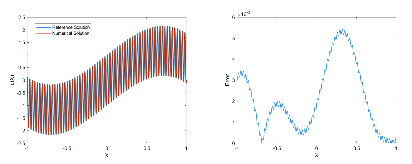
Next we solve problem (29) with $u(-1)=u(1)=0$ and $c>0$ , and a variable wave number $\omega(x)=\sin(mx^{2})$ , $m>0$ is a constant. As there is no explicit exact solution to this equation, the numerical solution obtained by a finite difference method with a fine mesh will be used as the reference solution.

We first choose $\lambda=2$ , $\mu=200$ , $c=0.9\lambda^{2}=3.6$ and $m=1$ in Eqn.(29), which corresponds to a high frequency external wave source and a low wave number with small background media inhomogeneity. In the coupled PhaseDNN, we choose $w_{m}\in\{1,2,3,4,200\}$ . Other training parameters are set to be similar as in the constant coefficient case. The numerical result of coupled phaseDNN and reference solution is shown in Fig. 9 and the absolute error is in the order of $O(10^{-3})$ .

Next, we choose $\lambda=100$ , $\mu=200$ , $c=0.1\lambda^{2}=1000$ and $m=100$ , which corresponds to a high frequency external wave source and a high wave number with larger background media inhomogeneity. $\omega_{m}$ is chosen to be $\{0,90,100,110,190,200,210\}$ . The learning result is shown in Fig. 10.

One can see that coupled PhaseDNN with least square residual minimization cannot solve the problem well. The right panel of Fig.10 shows the error concentrates on the $\pm\lambda$ component while the $\mu$ component converges quite good. The error of this method is mainly due to high wave number. This is an intrinsic difficulty of least square minimization based DNN method. The theoretical analysis of this phenomena will be done in a coming paper.

Next, we will apply the integral equation approach (34) (40) to this problem. The Green’s function to $u^{\prime\prime}+\lambda^{2}u=\delta(x-x^{\prime})$ with Dirichlet boundary condition $u(-1)=u(1)=0$ is given by

G(x{{}^{\prime}},x)=\left\{\begin{aligned} &\frac{(-\tan{\lambda}\cos{\lambda x^{{}^{\prime}}}+\sin{\lambda x^{{}^{\prime}}})(\tan{\lambda}\cos{\lambda x}+\sin{\lambda x})}{2\lambda\tan{\lambda}},s\leq x,\\ &\frac{(\tan{\lambda}\cos{\lambda x^{{}^{\prime}}}+\sin{\lambda x^{{}^{\prime}}})(-\tan{\lambda}\cos{\lambda x}+\sin{\lambda x})}{2\lambda\tan{\lambda}},s>x\end{aligned}\right.

(44)

With the same parameter setting, the numerical solution obtained by integral equation method is shown in Fig.11. The absolute error is in the order of $O(10^{-3})$ .

Figure 11: Numerical and reference solution of problem (29) using coupled phaseDNN and integral equation method.

\lambda=100

\mu=200

c=1000

and

m=100

. Left panel: The numerical solution with reference solution. Right panel: The difference between numerical solution and reference solution.

It can be seen that coupled PhaseDNN with the integral equation approach (34) (40) gives more accurate solution than that for the differential equation method and does not suffer from high wave number errors as in Fig.11.

4.2.3 Solving elliptic equation

We can also solve elliptic differential equation with high frequency external sources using the coupled PhaseDNN. We consider a test problem

\begin{cases}u^{\prime\prime}-\lambda^{2}u=-(\lambda^{2}+\mu^{2})\sin(\mu x),\\ u(-1)=u(1)=0,\end{cases}

(45)

which has an exact solution as

u(x)=-\frac{\sin\mu}{\sinh\lambda}\sinh(\lambda x)+\sin(\mu x).

(46)

We choose $\lambda=3$ , $\mu=250$ in Eqn. (45). To solve this equation, we set a coupled PhaseDNN with $\omega_{m}\in\{0,\mu\}$ . Each subnetwork is a fully connected DNN with 4 layers and 20 neurons in each layer. Accurate training result is shown in Fig. 12.

4.2.4 Coupled PhaseDNN for solving exterior wave scattering problem

We consider problem (31) with $\lambda=100$ , $\mu=200$ , $c=0.1\lambda^{2}$ . The variable coefficient $\omega(x)=\chi_{[-1,1]}(x)\sin(1-x^{2})$ , and $f(x)=\chi_{[-1,1]}(x)(\lambda^{2}-\mu^{2})(1-x^{2})\sin(\mu x)$ .

We first solve the problem with Robin boundary condition (32) by the coupled PhaseDNN for the differential equation. The real part of the solution is shown in Fig.13. We set each sub network in (24) to be a 1-20-20-20-20-1 DNN. Training data set is 3000 evenly spaced points in $[-2,2]$ . The training runs 3000 epochs with batchsize 600.

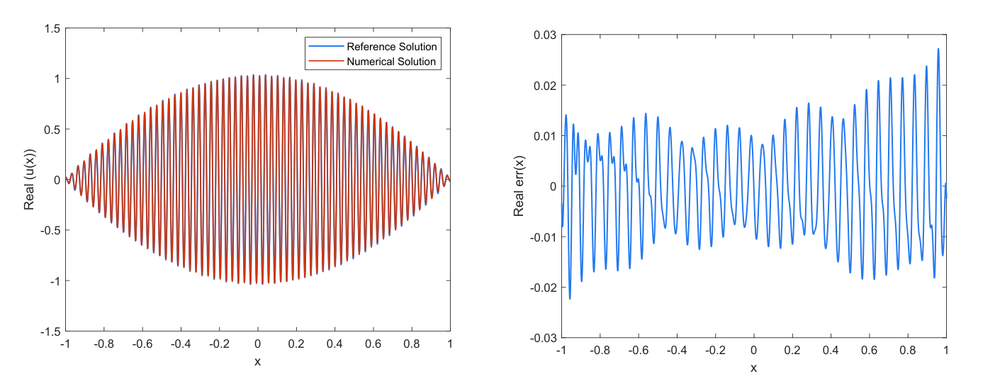
Again, this problem will be solved by the coupled PhaseDNN with the integral equation (34) (40), and the result is given in Fig.14. The training parameters are set similarly as for the differential equation method. Training runs 300 epochs. Better performance of the coupled PhaseDNN for the integral equation approach (34) (40), requiring much fewer training epochs, is shown, compared with the differential equation coupled PhaseDNN.

5 Conclusion

In this paper, we have proposed a phase shift DNN to learn high frequency information by using frequency shifts to convert the high frequency learning to low frequency one. As shown by various numerical tests, this approach increases dramatically the capability of the DNN as a viable tool for approximating high frequency functions and solutions of high frequency wave differential and integral equations in inhomogeneous media.

The optimization problem with the training of DNNs is complex and not much understood during the search of parameter spaces of the DNNs for a local or global minima. The specific structure of the proposed PhaseDNN seems to guide this search more efficiently than the common fully connected DNNs. Meanwhile, our numerical results also show that the PhaseDNN with integral equation formulation of the high frequency wave problems gives better accuracy to that with differential equations. These issues will be the subject of future theoretical analysis of the PhaseDNN. Also for future work, we will further develop the PhaseDNN to handle the high dimensionality problems from random inhomogeneous media in the wave propagations.

Appendix

In this appendix, we will show that under a condition that the weight of the input layer for each sub DNN $T_{m}(x)$ is small enough, coupled PhaseDNN is approximately equivalent to parallel PhaseDNN in approximating a function during training.

For simplicity, we only consider the 1-D case $d=1$ and assume $|\omega_{i}-\omega_{j}|=|i-j|\Delta k$ for all $1\leqslant i,j\leqslant M$ and some $\Delta k>0$ .

Generally, the Fourier transform of a target function $f(x)$ and DNN function $T(x)$ may not exists. However, as we are only interested in the target function in a compact domain $\Omega\subset\mathbb{R}^{d}$ . To avoid this technical problem in analysis, we choose a smooth mollifier function $\kappa(x)$ satisfies $\kappa(x)=1$ for $x\in\Omega$ and $\kappa(x)=0$ for $x\in\mathbb{R}^{d}\backslash\Omega^{\prime}$ , where $\Omega\subset\Omega^{\prime}\subset\mathbb{R}^{d}$ . We assume $f(x)\kappa(x)\in H^{r}$ and $T(x)\kappa(x)\in H^{r}$ for some $r\geq 1$ . This assumption ensures the existence of Fourier transform for $f(x)\kappa(x)$ and $T(x)\kappa(x)$ . For simplicity purpose, in the following text, we still use $f(x)$ and $T(x)$ to indicate $f(x)\kappa(x)$ and $T(x)\kappa(x)$ .

Although in practice, we usually use the real form of coupled phase DNN (24), in analysis, we prefer the complex form (21). Recall $T_{m}(x)$ in (21) is complex valued and each DNN $T_{m}$ in (21) can be written as $T_{m}(x)=u_{m}(\eta w_{m}x+b_{m})$ , where $\eta>0$ is a small parameter, and $u_{m}(t)$ are (complex valued) DNN functions except the input layer. Again, in general, $u_{m}(x)$ is not $\mathbb{L}^{2}$ function, however, as we are not interest in its behavior at infinity, we can multiply it by a smooth mollifier function $\kappa(x)$ s.t. $\kappa(x)=1$ in a compact domain $\Omega\subset\mathbb{R}$ and $\kappa(x)=0$ in $\mathbb{R}\backslash\Omega^{\prime}$ . Here, the compact domain $\Omega^{\prime}$ satisfies $\Omega\subset\Omega^{\prime}\subset\mathbb{R}$ . We assume the new function $u(x)\kappa(x)\in H^{r}(\mathbb{R})$ , $r\geq 1$ . For simplicity, in the following text, we still use $u(x)$ stands for the $H^{r}$ function $u(x)\kappa(x)$ . Without losing generality, we can assume $w_{m}\neq 0$ for all $1\leqslant m\leqslant M$ .

We know that $u_{m}(x,\theta)\in L^{2}(\mathbb{R})$ , where $\theta=\theta(t)$ , $t$ stands for training process. It is reasonable to assume that

Assumption 1.

During the training $t\in[0,T]$ , there is a constant $H>0$ s.t

H^{-1}<\inf_{t\in[0,T]}\left\|{u_{m}}\right\|_{2}\leqslant\sup_{t\in[0,T]}\left\|{u_{m}}\right\|_{2}<H

holds for any $1\leqslant m\leqslant M$ .

This assumption is reasonable because if $\left\|{u}\right\|_{2}$ has no upper bound means the training blows up while no positive lower bound means this term vanishes. The constant is uniform because $M$ is finite. Furthermore, we can assume

Assumption 2.

For any $\epsilon>0$ , there is constant $A>0$ s.t.

\int_{A}^{+\infty}|\hat{u}_{m}|^{2}\,\mathrm{d}k<\epsilon,\mbox{ and }\int_{-\infty}^{-A}|\hat{u}_{m}|^{2}\,\mathrm{d}k<\epsilon

holds for any $1\leqslant m\leqslant M$ and $t\in[0,T]$ .

It is straightforward to show that the Fourier transform of (21) yields

\hat{T}(k)=\sum_{m=1}^{M}\hat{T}_{m}(k-\omega_{m})=\sum_{m=1}^{M}\frac{1}{\eta|w_{m}|}\exp(-\frac{ib_{m}(k-\omega_{m})}{\eta w_{m}})\hat{u}_{m}(\frac{k-\omega_{m}}{\eta w_{m}}),

(47)

and

L(\theta)=\int_{-\infty}^{\infty}|\hat{f}-\hat{T}|^{2}\,\mathrm{d}k=\int_{-\infty}^{\infty}|\hat{f}|^{2}\,\mathrm{d}k-2Re\int_{-\infty}^{\infty}\hat{T}\bar{\hat{f}}\,\mathrm{d}k+\int_{-\infty}^{\infty}|\hat{T}|^{2}\,\mathrm{d}k.

(48)

In eqn. (48),

\int_{-\infty}^{\infty}|\hat{T}|^{2}\,\mathrm{d}k=\int_{-\infty}^{\infty}\sum_{m,n=1}^{M}\hat{T}_{m}(k-\omega_{m})\bar{\hat{T}}_{n}(k-\omega_{n})\,\mathrm{d}k.

We will show that under assumption 1 and 2, when $\eta\to 0$ ,

\frac{\int_{-\infty}^{\infty}|T_{m}(k-\omega_{m})||T_{n}(k-\omega_{n})|\,\mathrm{d}k}{\int_{-\infty}^{\infty}|T_{m}(k-\omega_{m})|^{2}\,\mathrm{d}k}\to 0

(49)

for all $m=1,2,\dots M$ and $n\neq m$ .

To this end, we first notice that

$\displaystyle\int_{-\infty}^{\infty}\|T_{m}(k-\omega_{m})\|^{2}\,\mathrm{d}k$	$\displaystyle=\frac{1}{\eta^{2}w_{m}^{2}}\int_{-\infty}^{\infty}\|\hat{u}_{m}(\frac{k-\omega_{m}}{\eta w_{m}})\|^{2}\,\mathrm{d}k$	(50)
	$\displaystyle=\frac{1}{\eta\left\|w_{m}\right\|}\int_{-\infty}^{\infty}\|\hat{u}_{m}(t)\|^{2}\,\mathrm{d}t$
	$\displaystyle=\frac{\left\\|{u_{m}}\right\\|_{2}^{2}}{\eta\left\|w_{m}\right\|}>\frac{1}{\eta H\left\|w_{m}\right\|}.$

At the same time,

$\displaystyle\int_{-\infty}^{\infty}\|T_{m}(k-\omega_{m})\|$	$\displaystyle\|T_{n}(k-\omega_{n})\|\,\mathrm{d}k$	(51)
	$\displaystyle=\frac{1}{\eta^{2}\left\|w_{m}\right\|\left\|w_{n}\right\|}\int_{-\infty}^{\infty}\|\hat{u}_{m}(\frac{k-\omega_{m}}{\eta w_{m}})\|\|\hat{u}_{n}(\frac{k-\omega_{n}}{\eta w_{n}})\|\,\mathrm{d}k$
	$\displaystyle=\frac{1}{\eta\left\|w_{n}\right\|}\int_{-\infty}^{\infty}\|\hat{u}_{m}(t)\|\|\hat{u}_{n}(\frac{w_{m}}{w_{n}}t+\frac{\omega_{m}-\omega_{n}}{\eta w_{n}})\|\,\mathrm{d}t$
	$\displaystyle=\frac{1}{\eta\left\|w_{n}\right\|}\left(\int_{-\infty}^{-A}+\int_{-A}^{A}+\int_{A}^{\infty}\right).$

Applying the Cauchy-Schwardz inequality, we can estimate the first integral by

$\displaystyle\int_{-\infty}^{-A}\|\hat{u}_{m}(t)\|$	$\displaystyle\|\hat{u}_{n}(\frac{w_{m}}{w_{n}}t+\frac{\omega_{m}-\omega_{n}}{\eta w_{n}})\|\,\mathrm{d}t$	(52)
	$\displaystyle\leqslant\left(\int_{-\infty}^{-A}\|\hat{u}_{m}(t)\|^{2}\,\mathrm{d}t\right)^{1/2}\left(\int_{-\infty}^{-A}\|\hat{u}_{n}(\frac{w_{m}}{w_{n}}t+\frac{\omega_{m}-\omega_{n}}{\eta w_{n}})\|^{2}\,\mathrm{d}t\right)^{1/2}$
	$\displaystyle\leqslant\sqrt{\epsilon\left\|\frac{w_{n}}{w_{m}}\right\|}\left\\|{\hat{u}_{n}}\right\\|_{2}<\epsilon\sqrt{\left\|\frac{w_{n}}{w_{m}}\right\|}H.$

Similarly, we can also estimate

\int^{\infty}_{A}|\hat{u}_{m}(t)||\hat{u}_{n}(\frac{w_{m}}{w_{n}}t+\frac{\omega_{m}-\omega_{n}}{\eta w_{n}})|\,\mathrm{d}t\leqslant\epsilon\sqrt{\left|\frac{w_{n}}{w_{m}}\right|}H.

(53)

For the second integral, we have

$\displaystyle\int_{-A}^{A}\|\hat{u}_{m}(t)\|$	$\displaystyle\|\hat{u}_{n}(\frac{w_{m}}{w_{n}}t+\frac{\omega_{m}-\omega_{n}}{\eta w_{n}})\|\,\mathrm{d}t$	(54)
	$\displaystyle\leqslant\left(\int_{-A}^{A}\|\hat{u}_{m}(t)\|^{2}\,\mathrm{d}t\right)^{1/2}\left(\int_{-A}^{A}\|\hat{u}_{n}(\frac{w_{m}}{w_{n}}t+\frac{\omega_{m}-\omega_{n}}{\eta w_{n}})\|^{2}\,\mathrm{d}t\right)^{1/2}$
	$\displaystyle\leqslant\sqrt{\left\|\frac{w_{n}}{w_{m}}\right\|}\left\\|{u_{m}}\right\\|_{2}\left(\int_{\frac{\|\omega_{m}-\omega_{n}\|}{\eta\|w_{n}\|}-\left\|\frac{w_{m}}{w_{n}}\right\|A}^{\frac{\|\omega_{m}-\omega_{n}\|}{\eta\|w_{n}\|}+\left\|\frac{w_{m}}{w_{n}}\right\|A}\left\|\hat{u}_{n}(t)\right\|^{2}\,\mathrm{d}t\right)^{1/2}.$

Since $n\neq m$ , $\omega_{m}-\omega_{n}\neq 0$ . When $\eta<\frac{\left|\omega_{m}-\omega_{n}\right|}{\left|w_{m}\right|+\left|w_{n}\right|}$ ,

\int_{\frac{|\omega_{m}-\omega_{n}|}{\eta|w_{n}|}-\left|\frac{w_{m}}{w_{n}}\right|A}^{\frac{|\omega_{m}-\omega_{n}|}{\eta|w_{n}|}+\left|\frac{w_{m}}{w_{n}}\right|A}\left|\hat{u}_{n}(t)\right|^{2}\,\mathrm{d}t<\int_{A}^{\infty}\left|\hat{u}_{n}(t)\right|^{2}\,\mathrm{d}t<\epsilon.

To choose a uniform $\eta$ , it is sufficient to set

\eta<\min_{m\neq n}\frac{\left|\omega_{m}-\omega_{n}\right|}{\left|w_{m}\right|+\left|w_{n}\right|}=\frac{\Delta k}{2\max_{m}\left|w_{m}\right|}>0.

Combining eqn (52), (53), (54) and (50), we can conclude that

\frac{\int_{-\infty}^{\infty}|T_{m}(k-\omega_{m})||T_{n}(k-\omega_{n})|\,\mathrm{d}k}{\int_{-\infty}^{\infty}|T_{m}(k-\omega_{m})|^{2}\,\mathrm{d}k}\to 0,(\eta\to 0)

holds for all $1\leqslant m\neq n\leqslant M$ . Thus, when $\eta$ is small enough, we can estimate

	$\displaystyle\int_{-\infty}^{\infty}\|\hat{T}\|^{2}\,\mathrm{d}k$	$\displaystyle=\int_{-\infty}^{\infty}\sum_{m,n=1}^{M}\hat{T}_{m}(k-\omega_{m})\bar{\hat{T}}_{n}(k-\omega_{n})\,\mathrm{d}k$		(55)
		$\displaystyle\approx\sum_{m=1}^{M}\int_{-\infty}^{\infty}\left\|\hat{T}_{m}(k-\omega_{m})\right\|^{2}\,\mathrm{d}k$		(55)

We can do decomposition of $\hat{f}(k)=\sum_{m=1}^{M}\hat{f}(k)\chi_{m}(k)=\sum_{m=1}^{M}\hat{f}_{m}$ , where $\chi_{m}(k)$ is the indicator function of interval $[\omega_{m}-\Delta k/2,\omega_{m}+\Delta k/2]$ . It is easy to see $|\hat{f}|^{2}=\sum_{m=1}^{M}|\hat{f}_{m}|^{2}$ and

\int_{-\infty}^{\infty}\hat{T}\bar{\hat{f}}\,\mathrm{d}k=\sum_{m,n=1}^{M}\int_{-\infty}^{\infty}\hat{T}_{m}(k-\omega_{m})\hat{f}_{n}(k)\,\mathrm{d}k.

With the same argument in proving eqn (49), we can also deduce that if $\hat{f}_{n}\neq 0$

\frac{\int_{-\infty}^{\infty}\left|\hat{T}_{m}(k-\omega_{m})\right||\hat{f}_{n}|\,\mathrm{d}k}{\int_{-\infty}^{\infty}\left|\hat{T}_{n}(k-\omega_{n})\right||\hat{f}_{n}|\,\mathrm{d}k}\to 0

(56)

for all $m=1,2,\dots,M$ and $n\neq m$ . Thus

\int_{-\infty}^{\infty}\hat{T}\bar{\hat{f}}\,\mathrm{d}k\approx\sum_{m=1}^{M}\int_{-\infty}^{\infty}\hat{T}_{m}(k-\omega_{m})\bar{\hat{f}}_{m}.

(57)

Substituting approximations (55) and (57) to loss function (48), a good approximation of loss function, when $\eta$ is small, is

$\displaystyle L(\theta)$	$\displaystyle\approx\int_{-\infty}^{\infty}\sum_{m=1}^{M}\left\|\hat{f}_{m}(k)\right\|^{2}-2Re\hat{T}_{m}(k-\omega_{m})\bar{\hat{f}}_{m}+\left\|\hat{T}_{m}(k-\omega_{m})\right\|^{2}\,\mathrm{d}k$	(58)
	$\displaystyle=\sum_{m=1}^{M}\int_{-\infty}^{\infty}\left\|\hat{f}_{m}(k)-\hat{T}_{m}(k-\omega_{m})\right\|^{2}\,\mathrm{d}k$
	$\displaystyle=\sum_{m=1}^{M}\int_{-\infty}^{\infty}\left\|\mathcal{F}^{-1}[\hat{f}_{m}(k+\omega_{m})]-T_{m}(x)\right\|^{2}\,\mathrm{d}x$
	$\displaystyle=\sum_{m=1}^{M}\int_{-\infty}^{\infty}\left\|e^{-i\omega_{m}x}\mathcal{F}^{-1}[\hat{f}_{m}](x)-T_{m}(x)\right\|^{2}\,\mathrm{d}x$

Here, $e^{-i\omega_{m}x}\mathcal{F}^{-1}[\hat{f}_{m}](x)$ is exactly the $f^{\text{shift}}_{m}(x)$ in (14), whose support in frequency space is $[-\Delta k/2,\Delta k/2]$ . Hence, the total loss function $L(\theta)$ is approximately the sum of $M$ individual DNNs $T_{m}$ that learn $f^{\text{shift}}_{m}(x)$ , separately.

References

[1] Bochev PB, Gunzburger MD. Finite element methods of least-squares type. SIAM review. 1998;40(4):789-837.
[2] Cai, Wei, Xiaoguang Li, Lizuo Liu, PhaseDNN - A Parallel Phase Shift Deep Neural Network for Adaptive Wideband Learning, arxiv 1905.01389, May 3, 2019.
[3] Brandt, Achi. Multi-level adaptive solutions to boundary-value problems. Mathematics of computation 31.138 (1977): 333-390.
[4] Daubechies, Ingrid. Ten lectures on wavelets. Vol. 61. Siam, 1992.
[5] E, Weinan, and Bing Yu. ”The Deep Ritz method: A deep learning-based numerical algorithm for solving variational problems.” Communications in Mathematics and Statistics 6.1 (2018): 1-12.
[6] Jiang BN, Povinelli LA. Least-squares finite element method for fluid dynamics. Computer Methods in Applied Mechanics and Engineering. 1990 Jul 1;81(1):13-37.
[7] Luo, Tao and Ma, Zheng and Xu, Zhi-Qin John and Zhang, Yaoyu. Theory of the Frequency Principle for General Deep Neural Networks. arXiv preprint arXiv:1906.09235 (2019)
[8] Raissi, Maziar and Perdikaris, Paris and Karniadakis, George E. Physics-informed neural networks: A deep learning framework for solving forward and inverse problems involving nonlinear partial differential equations. Journal of Computational Physics 378(2019): 686-707
[9] Goodfellow, Ian and Bengio, Yoshua and Courville, Aaron. Deep learning. MIT press(2016)
[10] Xu, Zhi-Qin John, Understanding training and generalization in deep learning by Fourier analysis, arXiv:1808.04295, November, 2018.
[11] Xu, Zhi-Qin John, Yaoyu Zhang, Tao Luo, Yanyang Xiao, and Zheng Ma. Frequency Principle: Fourier Analysis Sheds Light on Deep Neural Networks. arXiv preprint arXiv:1901.06523 (2019).

$\displaystyle\int_{-\infty}^{\infty}\|T_{m}(k-\omega_{m})\|^{2}\,\mathrm{d}k$	$\displaystyle=\frac{1}{\eta^{2}w_{m}^{2}}\int_{-\infty}^{\infty}\|\hat{u}_{m}(\frac{k-\omega_{m}}{\eta w_{m}})\|^{2}\,\mathrm{d}k$	(50)
	$\displaystyle=\frac{1}{\eta\left\|w_{m}\right\|}\int_{-\infty}^{\infty}\|\hat{u}_{m}(t)\|^{2}\,\mathrm{d}t$
	$\displaystyle=\frac{\left\\|{u_{m}}\right\\|_{2}^{2}}{\eta\left\|w_{m}\right\|}>\frac{1}{\eta H\left\|w_{m}\right\|}.$

$\displaystyle\int_{-\infty}^{\infty}\|T_{m}(k-\omega_{m})\|$	$\displaystyle\|T_{n}(k-\omega_{n})\|\,\mathrm{d}k$	(51)
	$\displaystyle=\frac{1}{\eta^{2}\left\|w_{m}\right\|\left\|w_{n}\right\|}\int_{-\infty}^{\infty}\|\hat{u}_{m}(\frac{k-\omega_{m}}{\eta w_{m}})\|\|\hat{u}_{n}(\frac{k-\omega_{n}}{\eta w_{n}})\|\,\mathrm{d}k$
	$\displaystyle=\frac{1}{\eta\left\|w_{n}\right\|}\int_{-\infty}^{\infty}\|\hat{u}_{m}(t)\|\|\hat{u}_{n}(\frac{w_{m}}{w_{n}}t+\frac{\omega_{m}-\omega_{n}}{\eta w_{n}})\|\,\mathrm{d}t$
	$\displaystyle=\frac{1}{\eta\left\|w_{n}\right\|}\left(\int_{-\infty}^{-A}+\int_{-A}^{A}+\int_{A}^{\infty}\right).$

$\displaystyle\int_{-\infty}^{-A}\|\hat{u}_{m}(t)\|$	$\displaystyle\|\hat{u}_{n}(\frac{w_{m}}{w_{n}}t+\frac{\omega_{m}-\omega_{n}}{\eta w_{n}})\|\,\mathrm{d}t$	(52)
	$\displaystyle\leqslant\left(\int_{-\infty}^{-A}\|\hat{u}_{m}(t)\|^{2}\,\mathrm{d}t\right)^{1/2}\left(\int_{-\infty}^{-A}\|\hat{u}_{n}(\frac{w_{m}}{w_{n}}t+\frac{\omega_{m}-\omega_{n}}{\eta w_{n}})\|^{2}\,\mathrm{d}t\right)^{1/2}$
	$\displaystyle\leqslant\sqrt{\epsilon\left\|\frac{w_{n}}{w_{m}}\right\|}\left\\|{\hat{u}_{n}}\right\\|_{2}<\epsilon\sqrt{\left\|\frac{w_{n}}{w_{m}}\right\|}H.$

$\displaystyle\int_{-A}^{A}\|\hat{u}_{m}(t)\|$	$\displaystyle\|\hat{u}_{n}(\frac{w_{m}}{w_{n}}t+\frac{\omega_{m}-\omega_{n}}{\eta w_{n}})\|\,\mathrm{d}t$	(54)
	$\displaystyle\leqslant\left(\int_{-A}^{A}\|\hat{u}_{m}(t)\|^{2}\,\mathrm{d}t\right)^{1/2}\left(\int_{-A}^{A}\|\hat{u}_{n}(\frac{w_{m}}{w_{n}}t+\frac{\omega_{m}-\omega_{n}}{\eta w_{n}})\|^{2}\,\mathrm{d}t\right)^{1/2}$
	$\displaystyle\leqslant\sqrt{\left\|\frac{w_{n}}{w_{m}}\right\|}\left\\|{u_{m}}\right\\|_{2}\left(\int_{\frac{\|\omega_{m}-\omega_{n}\|}{\eta\|w_{n}\|}-\left\|\frac{w_{m}}{w_{n}}\right\|A}^{\frac{\|\omega_{m}-\omega_{n}\|}{\eta\|w_{n}\|}+\left\|\frac{w_{m}}{w_{n}}\right\|A}\left\|\hat{u}_{n}(t)\right\|^{2}\,\mathrm{d}t\right)^{1/2}.$

$\displaystyle L(\theta)$	$\displaystyle\approx\int_{-\infty}^{\infty}\sum_{m=1}^{M}\left\|\hat{f}_{m}(k)\right\|^{2}-2Re\hat{T}_{m}(k-\omega_{m})\bar{\hat{f}}_{m}+\left\|\hat{T}_{m}(k-\omega_{m})\right\|^{2}\,\mathrm{d}k$	(58)
	$\displaystyle=\sum_{m=1}^{M}\int_{-\infty}^{\infty}\left\|\hat{f}_{m}(k)-\hat{T}_{m}(k-\omega_{m})\right\|^{2}\,\mathrm{d}k$
	$\displaystyle=\sum_{m=1}^{M}\int_{-\infty}^{\infty}\left\|\mathcal{F}^{-1}[\hat{f}_{m}(k+\omega_{m})]-T_{m}(x)\right\|^{2}\,\mathrm{d}x$
	$\displaystyle=\sum_{m=1}^{M}\int_{-\infty}^{\infty}\left\|e^{-i\omega_{m}x}\mathcal{F}^{-1}[\hat{f}_{m}](x)-T_{m}(x)\right\|^{2}\,\mathrm{d}x$

A Phase Shift Deep Neural Network for High Frequency Approximation and Wave Problems Thanks: to be submitted to SISC.

Abstract

keywords

1 Introduction

2 A parallel phase shift DNN (PhaseDNN) for high frequency approximation

Theorem 1.

2.1 Frequency selection kernel ϕj∨​(x)\phi_{j}^{\vee}(x)

2.2 A parallel phase shift DNN (PhaseDNN) algorithm

3 A coupled PhaseDNN

3.1 Approximating functions

Remark 1.

3.2 Solving differential equations through least square residual minimization

3.3 Solving integral equations for exterior Helmholtz problems

Remark 2.

4 Numerical results

4.1 Approximation of functions with PhaseDNN

4.1.1 Parallel PhaseDNN

4.1.2 Coupled PhaseDNN

Remark 3.

4.2 Coupled PhaseDNN for solving high frequency wave problems

4.2.1 Helmholtz equation with constant wave numbers

4.2.2 Helmholtz equation with variable wave numbers

4.2.3 Solving elliptic equation

4.2.4 Coupled PhaseDNN for solving exterior wave scattering problem

5 Conclusion

Appendix

Assumption 1.

Assumption 2.

References

2.1 Frequency selection kernel $\phi_{j}^{\vee}(x)$