Three-dimensional advective–diffusive boundary layers in open channels with parallel and inclined walls
Abstract
We study the steady laminar advective transport of a diffusive passive scalar released at the base of narrow three-dimensional longitudinal open channels with non-absorbing side walls and rectangular or truncated-wedge-shaped cross-sections. The scalar field in the advective–diffusive boundary layer at the base of the channels is fundamentally three-dimensional in the general case, owing to a three-dimensional velocity field and differing boundary conditions at the side walls. We utilise three-dimensional numerical simulations and asymptotic analysis to understand how this inherent three-dimensionality influences the advective-diffusive transport as described by the normalised average flux, the Sherwood or Nusselt numbers for mass or heat transfer, respectively. We show that is well approximated by an appropriately formulated two-dimensional calculation, even when the boundary layer structure is itself far from two-dimensional. This is a key and novel results which can significantly simplify the modelling of many laminar advection–diffusion scalar transfer problems. The different transport regimes found depend on the channel geometry and a characteristic Péclet number based on the ratio of the cross-channel diffusion time and the longitudinal advection time. We develop asymptotic expressions for in the various limiting regimes, which mainly depend on the confinement of the boundary layer in the lateral and base-normal directions. For we recover the classical Lévêque solution with a cross-channel-averaged shear rate , , for both geometries despite strongly curved boundary layers; for parallel walls a secondary regime with is found for . In the case of truncated wedge channels, further regimes are identified owing to curvature effects, which we capture through a curvature-rescaled Péclet number , with the opening angle of the wedge. For , the Sherwood number appears to follow . In all cases, we offer a comparison between our three-dimensional simulations, the asymptotic results and our two-dimensional simplifications, and can thus quantify the error in the flux from the simplified calculations. Our findings are relevant to heat and mass transfer applications in confined U-shaped or V-shaped channels such as for the decontamination and cleaning of narrow gaps or transport processes in chemical or biological microfluidic devices.
1 Introduction
The advective–diffusive transfer of a scalar (e.g. mass or heat) at solid–liquid boundaries in laminar channel flows is a fundamental transport phenomenon found in numerous applications. Mass transfer applications include: chemical (Zhang et al. 1996; Gervais and Jensen 2006; Kirtland et al. 2009) and biological (Vijayendran et al. 2003; Squires et al. 2008; Hansen et al. 2012) microfluidic reactors and sensors, porous microfluidic channels and membranes (Dejam 2019; Kou and Dejam 2019), membrane extraction techniques (Jönsson and Mathiasson 2000; Marczak et al. 2006), micro-mixers (Kamholz et al. 1999; Ismagilov et al. 2000; Kamholz and Yager 2001; Kamholz and Yager 2002; Stone et al. 2004; Jiménez 2005; Capretto et al. 2011), membraneless electrochemical fuel cells (Ferrigno et al. 2002; Cohen et al. 2005; Braff et al. 2013), cross-flow membrane filtration Porter 1972; Bowen and Jenner 1995; Visvanathan et al. 2000; Herterich et al. 2015, crystal dissolution (Bisschop and Kurlov 2013), aquifer remediation (Borden and Kao 1992; Dejam et al. 2014; Kahler and Kabala 2016), and cleaning Wilson 2005; Fryer and Asteriadou 2009; Lelieveld et al. 2014; Pentsak et al. 2019 and decontamination Fitch et al. 2003; Settles 2006 in channels. Heat transfer applications include: film cooling (Acharya and Kanani 2017), heat exchangers (Kakaç and Liu 2002; Ayub 2003), and cooling and heating in micro-channels (Sobhan and Garimella 2001; Avelino and Kakaç 2004). Determining and predicting the advection-enhanced scalar flux at the transfer boundary as a function of geometry, flow and scalar properties is highly desired in these problems. It allows assessment of the performance of the overall scalar transport. Also, scalar transfer at the boundary is often a critical rate-limiting step compared to other processes, particularly for mass transfer owing to low mass diffusivities compared to advection or reaction rates as commonly found in applications (Gervais and Jensen 2006; Squires et al. 2008; Kirtland et al. 2009, e.g.).
Solving the scalar transport problem in high-Péclet number flows near boundaries was pioneered by the theoretical works of Graetz (Graetz 1885), Nusselt (Nusselt 1916) and Lévêque (Lévêque 1928) for two-dimensional problems. They give analytical or scaling predictions for the scalar flux and the associated non-dimensional transfer coefficient: the Sherwood and Nusselt numbers for mass and heat transfer, respectively. Mass transfer problems have benefited from progress in the understanding of heat transfer (Bejan 2013, e.g.), since heat and mass transfer problems are equivalent when both scalars are passive or have the same properties. Henceforth, we refer to the generic scalar non-dimensional transfer coefficient as the Sherwood number, , for simplicity, as we assume a passive scalar in this study. This assumption implies that the scalar transport equation and the governing equation for the flow are not fully coupled, such that the flow is independent of the tracer concentration, whereas the concentration field depends on the flow field. Thus, buoyancy or temperature changes that could affect the flow field are beyond the scope of this study. Nevertheless, our results apply to analogous heat transfer problems provided that the temperature difference is sufficiently small. We will revisit these assumptions and their effect on the results in section 7.
Although numerical simulations can now solve almost any scalar transport problem with complex boundary conditions or geometries, the ease of use of simple theoretical predictions is still highly valuable for a broad range of applications. Theoretical models mostly rely on the key, widely-used simplifying assumption that the scalar transport problems modelled can be approximated by two-dimensional problems. Transfer problems in steady axisymmetric channel flows with uniform lateral boundary conditions (e.g. Dirichlet or Neumann) can directly use the two-dimensional axisymmetric theoretical results of Graetz: (Bejan 2013, e.g.), with the Reynolds number, the Schmidt number, and the ratio of the channel diameter and the length of the scalar transfer area. (Throughout this paper, hats denote dimensional quantities and dimensionless quantities remain undecorated.) The positive exponents , and vary depending on the flow profile (e.g. uniform or shear flow) and regime (laminar or turbulent), the wall roughness and whether the diffusive and momentum boundary layers are full developed or not. Non-axisymmetric three-dimensional problems, such as rectangular channel flows, also rely on empirical or asymptotic correlations based on Graetz’ two-dimensional results by modifying the Sherwood number such that: (Gekas and Hallström 1987; Bowen and Jenner 1995, e.g.). The three-dimensional variations of the scalar field from a two-dimensional axisymmetric profile are thus captured by the ratio in the relationship above, where the hydraulic diameter accounts for non-circular channel cross-section. The key underlying assumption allowing non-axisymmetric three-dimensional problems to be modelled as two-dimensional axisymmetric problems is that the scalar boundary condition is uniform, i.e. not mixed, at the side walls. This assumption has proven useful to many mass (Gekas and Hallström 1987; Bowen and Jenner 1995, e.g. reviews) and heat (Sobhan and Garimella 2001; Ayub 2003; Avelino and Kakaç 2004, e.g. reviews) transfer problems.
Three-dimensional channel flows with mixed or differing scalar boundary conditions at the side walls can also be simplified to two-dimensional planar problems provided that the side walls with different boundary conditions have a negligible effect on the overall transfer flux. This assumption is typically used when channel widths are larger than heights (Squires et al. 2008; Braff et al. 2013, e.g.). Two-dimensional planar problems can then use advanced mathematical techniques such as potential flow and conformal mapping (Bazant 2004; Choi et al. 2005), which provide analytical or semi-analytical solutions for any complex (planar) geometries.
However, not all transport problems can be a priori reduced to simple axisymmetric or planar two-dimensional problems. Many problems possess three-dimensional flow and scalar fields owing to three-dimensional geometries and differing lateral boundary conditions, thus rendering analytical progress intractable. The main objective of this study, to predict the scalar flux and the Sherwood number as a function of the flow, scalar properties and geometry, requires us to analyse the impact of three-dimensional effects. We focus on three-dimensional transport problems in laminar steady fully-developed longitudinal open channel flows with generic rectangular or truncated wedge geometries. As depicted in figure 1, we study the case where we have different scalar boundary conditions at the side walls with: fixed Dirichlet boundary condition at the base of the channel, and no-flux boundary condition on all other boundaries. Transport occurs at high Péclet numbers such that a scalar boundary layer develops from the base of the channel. We define the channel aspect ratio as the ratio of the characteristic channel ‘height’ , in the direction perpendicular to the base of the channel, to the characteristic channel width , in the lateral direction. Three-dimensional effects are more significant when the channel aspect ratio is large and the scalar boundary layer is narrowly confined in the lateral direction. We describe these geometries as ‘open channels’ in the sense that when the channel has a finite height a free-slip boundary condition is assumed at the boundary opposite the base, and require this boundary to have a width larger or equal to that of the base. As illustrated in figure 1, the contour lines of the scalar field in cross-sections of the channels can be strongly curved, whilst the profiles develop in the longitudinal direction. This is due to the no-slip and no-flux boundary conditions (for the velocity and scalar, respectively) on the near side walls.

The problem considered here is a complex three-dimensional transport problem which has received little attention in the literature for various reasons. For example, many engineering applications in heat and mass transfer seek to maximise the interfacial transfer and thus tend to use geometrical design with aspect ratios corresponding to a “thin layer”, such that the width of the channel is much larger than its height . A large number of studies in the heat and mass transfer literature have thus focussed on enhancing the scalar transfer (i.e. the Sherwood number, , or the Nusselt number) in the small aspect ratio limit . However, the main novelty of our study is to focus on the opposite limit, or the “narrow channel” limit, where is naturally reduced due to confinement effects. This is less attractive for most engineering applications, which may explain why much less research has been done in the narrow channel limit. Importantly, in the narrow channel limit traditional two-dimensional approaches (Graetz 1885; Nusselt 1916; Lévêque 1928; Gekas and Hallström 1987; Bowen and Jenner 1995; Sobhan and Garimella 2001; Ayub 2003; Avelino and Kakaç 2004; Squires et al. 2008; Braff et al. 2013; Bejan 2013; Dejam et al. 2014; Kou and Dejam 2019; Dejam 2019, e.g.) that generally work in the thin layer limit cannot be used a priori since the flow and scalar fields are both inherently three-dimensional. This is the central point that motivates our study and which should be of interest to interfacial transfer problems where three-dimensional effects cannot be neglected.
The scenario shown in figure 1 closely models mass transfer applications in narrow spaces such as the cleaning and decontamination of gaps, cracks and fractures. This kind of cleaning problems exist in most industrial activities and are of particular concern in the food (Wilson 2005; Fryer and Asteriadou 2009; Lelieveld et al. 2014), chemical (Pentsak et al. 2019), pharmaceutical and cosmetic industries, where purity, hygiene and cleanliness are essential. This scenario is also relevant to the decontamination of toxic liquid materials trapped in confined channels where the flow is laminar (Fitch et al. 2003; Settles 2006). There are also potential applications to the pore-scale modelling of mass transfer phenomena in porous media, for instance in the context of aquifer remediation (Borden and Kao 1992; Kahler and Kabala 2016), if the micropores have a rectangular or truncated-wedge geometry. Another application is for the transport of ions in membraneless electrochemical cells. In this last case, to obtain the ion flux and deduce the current produced by the fuel cell, Braff et al. 2013 assumed a two-dimensional plug flow between electrodes in large aspect ratio channels in order to simplify the ion transport problem. However, the laminar flow in this geometry is fundamentally three-dimensional, also resulting in a three-dimensional ion concentration field owing to differing boundary conditions at the side walls. Our study provides a posteriori justification for the two-dimensional assumption made by Braff et al. 2013 and quantifies the associated error. The impact of three-dimensional effects has also been reported in microfluidic channels such as the T-sensor (Kamholz et al. 1999; Ismagilov et al. 2000; Kamholz and Yager 2001; Kamholz and Yager 2002; Stone et al. 2004). Jiménez 2005 showed with numerical and asymptotic techniques that shear flows near the no-flux and no-slip solid boundaries at the side walls lead to wall boundary layers. His results confirmed the power-laws found by Kamholz and Yager 2002 for the far-field region but not the initial square-root power-law. Jiménez 2005 also observed that, compared to the well-known case of longitudinal diffusion in a tube (Taylor 1953, ‘Taylor dispersion’;), the impact of the wall boundary layers on the effective mass transport is weak, the spreading rate changing by less than between the near and far-field regions.
To achieve our objective of understanding mass transport, we use asymptotic analysis and numerical simulations to determine the main impact of three-dimensional effects. We seek to elucidate the different regimes that exist and what controls the transition between them, and to demonstrate that in each case an appropriate two-dimensional model can be developed that provides a good approximation to . These findings have important theoretical and practical implications. Theoretically, it could enable the use of more advanced two-dimensional mathematical techniques in the case of more complex longitudinal profiles of the channel geometry (Bazant 2004; Choi et al. 2005). Practically, it enables computation of transfer fluxes in complex three-dimensional applications using simpler and faster techniques, whilst having clear estimates of the error made. This is particularly useful for end-users who may not have access to sophisticated computational tools or methods.
We begin by defining the problem in §2. In §3 we solve Stokes’ equation to obtain an analytical solution for the three-dimensional velocity field in rectangular channels with parallel walls and truncated-wedge channels with angled walls. We introduce the three-dimensional scalar transport problem and a two-dimensional cross-channel averaged formulation in §4. For channels with parallel walls, we use scaling arguments to obtain similarity solutions for the flux in cases where the diffusive boundary layer is much thinner (§5.1) or much thicker (§5.2) than the channel width. In §5.3, vertical confinement effects are studied through a depth-averaged advection–diffusion equation. In §5.4 and §5.5, three-dimensional numerical solutions of the transport problem demonstrate that two-dimensional results give accurate predictions for the Sherwood number across all Péclet numbers, including those where asymptotic approaches are not valid. In §6.1, we study the thin boundary layer regime for the truncated wedge geometry and show asymptotically that the opening wedge geometry leads to a small increase in the flux compared to the parallel wall geometry. In §6.2, thick boundary layers are studied for the wedge geometry, revealing a much more complex behaviour due to the impact of the opening angle on diffusion through curvature effects and advection. In §6.3, vertical confinement effects are studied for the truncated wedge geometry. In §6.4 and §6.5, three-dimensional numerical results for the truncated wedge geometry show that appropriate two-dimensional results give accurate predictions for the mass transfer in this geometry across all Péclet numbers studied and for small opening angles. A more complex dependence with Péclet number and geometry is found for the thick boundary layer regime. We also demonstrate the importance of a curvature-rescaled Péclet number in this regime. In §7, we discuss implications of our results for practical applications such as cleaning and decontamination in confined channels. In §8 and table 2, we summarize all our scaling and asymptotic results for the Sherwood number in the various regimes identified.

2 Model description
We model the steady advective–diffusive transport of a passive scalar released from an area of length in the flow direction and width . The release area, at the base of an infinitely long channel, is assumed to have zero thickness and have no effect on the velocity field. We study two generic three-dimensional geometries: a rectangular channel with parallel walls of arbitrary width and arbitrary height (figure 2, top row); and a channel forming a truncated wedge with a base in the form of an arc of a circle and flat side walls (figure 2, bottom row). (Here we use the term ‘height’ to represent the normal distance between the base and its opposite boundary or ‘top boundary’ without reference to the direction of gravity.) The opening angle of the wedge is and the arc length at the base of the channel is , with the truncation radius. In this study, we generally focus on the case of narrow channels, . However, our problem formulation is sufficiently general so that we are also able to discuss some results for and .
For rectangular channels with parallel walls, we use Cartesian coordinates , where denotes the streamwise coordinate, the direction normal to the channel base, and the cross-channel direction. The origin of the axes is placed at the intersection of the planes , the onset of the release area, , the base of the channel, and , the channel mid-plane. We refer to this geometry as a parallel-wall channel hereafter.
For truncated wedges with angled walls, we use cylindrical coordinates , where denotes the streamwise coordinate, the direction perpendicular to the base of the channel, the azimuthal direction. The origin is placed at the intersection between the plane , the onset of the area of release, and the axis , the edge of the wedge before truncation. For small angles , the curvature of the base could be neglected and the base of the channel considered flat, thus approximating the channel sketched in figure 1. We refer to this geometry as a truncated wedge hereafter.
The steady low-Reynolds-number open flow (see §3) in either form of channel is taken as unidirectional and independent of . The cross-sectional structure is controlled by the combination of the no-slip boundary conditions (see figure 2(a)) on the side walls and base of the channel, and an assumed stress-free condition at the top located at or . The top boundary condition is an approximation for a liquid–gas interface, which could be curved due to surface tension effects. Surface tension and curvature effects at the top boundary are neglected in this study.
The passive scalar transport with concentration is modelled using a steady advection–diffusion equation (see §4). The area of release has a fixed concentration (with a fixed background concentration) over the region given by , and for parallel-wall channels. Similarly, the area of release for truncated wedges is over , and . These regions are shown in figure 2(b,c) for parallel-wall channels (top row) and wedges (bottom row), respectively. All the channel walls have a no-flux boundary condition, except for the area of release. In cases where we consider an infinite fluid layer thickness, we assume at or . Otherwise, for a finite fluid layer thickness, we impose a no-flux boundary condition at or . Upstream, we impose for , and downstream, for .
3 Flow field
We assume an incompressible Stokes’ flow. Since the tracer is assumed passive, the governing equation for the fluid flow is independent of the tracer concentration. From the boundary conditions shown in figure 2, by symmetry, the flow field has only a streamwise component , which depends on and (respectively and for truncated wedges). The flow is driven by a constant streamwise gradient in the non-hydrostatic component of the pressure , which could be created by gravity for instance. Thus, the flow is three-dimensional in both geometries. Since we want to analyse three-dimensional effects on the scalar transport, it is important to capture the dependence of the flow with both coordinates. We non-dimensionalise spatial variables with the channel width or base arc length , the length scale for the flow at the channel base,
| (1) |
with the distance from the base of the truncated wedge, similar to . (Since the flow is independent of , we defer its non-dimensionalisation until §4.) All velocities are non-dimensionalised with the characteristic velocity , with the dynamic viscosity. The factor of preserves the intuitive physical meaning of the cross-channel averaged velocity in channels with parallel walls far away from the base.
3.1 Flow field in channels with parallel walls
The dimensionless Stokes equation for the flow in channels with parallel walls is
| (2) |
for , , with boundary conditions (figure 2, top row)
| (3) |
The solution of this inhomogeneous problem is described by the infinite series
| (4) |
where the eigenvalues and coefficients are, for all integers ,
| (5) |
The velocity (4) is shown in figure 3(a) for , truncated after 1000 terms. The flow is clearly three-dimensional near the base of the channel owing to the influence of the solid boundaries on three sides. However, for , the influence of the solid base decreases and the velocity field tends to a two-dimensional Poiseuille profile
| (6) |
valid only for . For , the flow is influenced by the base and , where is the dimensionless shear rate at . In general, the shear rate is
| (7) |
The dependence of with is important for . For , is uniform and approaches the semi-parabolic Nusselt film limit in the interior of the channel, owing to vertical confinement effect, with a dependence with limited to the corners, . Although (7) contains as a parameter, for the cross-channel average of the shear rate appears to be independent of and approaches asymptotically rapidly (see figure 3(a), appendix A). This is related to the fact that we impose a constant streamwise pressure gradient to drive the flow in the channel.
We also plot the cross-channel averaged velocity , with , in figure 3(c) (solid grey line), along with the two asymptotic limits: for and for . When analysing the scalar transport in the next sections, we will decompose the velocity such that , where and . Thus, three-dimensional effects related to the flow are contained in the cross-channel variation velocity .

3.2 Flow field in a truncated wedge channel
The dimensionless Stokes equation for the flow in truncated wedge channels is
| (8) |
for , , with boundary conditions (figure 2, bottom row)
| (9) |
Similar to parallel channels (see §3.1), the solution for the velocity is three-dimensional,
| (10) |
where the eigenvalues and the coefficients are, for all integers ,
| (11) | |||||
| (12) |
In figure 3(b) we show contour plots of the velocity (10) in a channel with , (see table 3 in appendix B for the number of eigenvalues used). For small opening angles, the flow field is similar to parallel channels (figure 3a). Far away from the top and base boundaries but closer to the side walls, for , (8) simplifies to , which gives, at leading order,
| (13) |
In contrast with the far-field velocity in parallel channels (see (6)), the far-field velocity in truncated wedges remains three-dimensional, except in the limit .
We plot in figure 3(c,d) the cross-channel averaged velocity , with , for opening angles (black solid line), (black dash-dotted line), and (black dashed line) for (c) and (d). Note that the noticeable change in slope for near for and 0.2 is due to the no-stress boundary condition at the top. Near the base, for , , similar to parallel channels, whilst in the far field , characteristic of a far-field flow in a narrow wedge. The shear rate at the base of the channel is given by
| (14) |
The dependence on vanishes in the interior of the channel for , owing to radial confinement effects, where it is limited to the corners, . The cross-channel average depends on and . For , , rapidly approaches the value for parallel channels: . For larger , , is approximately: 3.47 for , 4.00 for , and 8.68 for , see also appendix A and figure 3(b).
We will use the decomposition , with and ), in the next sections to study the impact of the three-dimensional cross-channel azimuthal variations on scalar transport in wedges.
4 Scalar transport
As noted in §1, the objective of this work is to determine the impact of three-dimensional effects on the flux of a passive scalar released from the base of a channel flow in the two geometries described in figure 2. The steady transport of a passive scalar is governed by the general advection–diffusion equation, assuming Fick’s law for molecular diffusion. We focus on the case where the scalar concentration field forms a slender diffusive boundary layer that develops in the direction such that , with a characteristic diffusive boundary layer thickness, a characteristic streamwise velocity at , and the scalar diffusivity. This implies that streamwise diffusion is negligible (Bejan 2013). As in (1), we use and as non-dimensionalising quantities. We also use the following non-dimensionalisation
| (15) |
where has been rescaled with the Péclet number . We choose as the characteristic length scale for the transport problem since the ratio between the diffusive boundary layer thickness and the gap width is key to describe the different regimes for the scalar transport and resulting flux. The advection–diffusion equation for parallel channels is then
| (16) |
for , , , with boundary conditions (figure 2)
| (17a) | ||||
| (17b–d) | ||||
| (17e,f) |
For truncated wedge channels, the governing advection–diffusion equation is
| (18) |
for , , , with boundary conditions (figure 2)
| (19a) | ||||
| (19b–d) | ||||
| (19e,f) |
The concentration field and resulting flux can be fully determined by solving (16) and (18) for using the velocity defined in (4) and (10), respectively.
In regimes dominated by cross-channel diffusion, we use the cross-channel average of (16) and (18) to determine the cross-channel averaged concentration and the flux. As introduced previously, we use and , where overbars denote cross-channel averages (along the -direction for parallel channels and along the -direction for wedges), and primes indicate cross-channel variations. We obtain for parallel channels
| (20) |
for , , with boundary conditions
| (21a–d) |
For truncated wedge channels we obtain
| (22) |
for , , with boundary conditions
| (23a–d) |
In both geometries, concentration iso-surfaces are in general three-dimensional. Owing to the boundary conditions, concentration profiles at a given are curved upwards. The effect of curved concentration profiles, combined with curved velocity profiles (as shown in figure 3), is captured by the fluctuation flux in (20) and (22). If or are small, this term may be negligible and the equations become two-dimensional. Otherwise, this term can either enhance or reduce the overall transport and flux. We investigate the effect of the three-dimensional fluctuation flux in detail in the next sections by considering the different limits for the ratio .
5 Channels with parallel walls
5.1 Thin boundary layer regime,
If , we can use the Lévêque approximation (Lévêque 1928) in the diffusive boundary layer, for (Glasgow 2010, for a discussion in English of some of Lévêque’s main results see ). The base shear rate is a function of , with a small dependence on (see (7)). The advection–diffusion equation (16) becomes
| (24) |
The different terms in (24) scale such that
| (25) |
where selects whichever of and is dominant. The dominant balance is in the diffusive boundary layer, resulting in the well-known Lévêque problem (Lévêque 1928) at leading order,
| (26) |
where the boundary conditions (4a–c) apply. Although , the problem remains three-dimensional as for each ‘slice’ depends parametrically on . We designate this modified Lévêque problem as the ‘slice-wise problem’ hereafter. The scaling (25) also suggests that the characteristic Péclet number in this problem is
| (27) |
The rescaled Péclet number compares the diffusion time across the channel width with the advection time along the length of release area . Thus, the diffusive boundary layer thickness is in the Lévêque regime, which is valid for .
A similarity solution for (26) exists with similarity variable (Bejan 2013)
| (28) |
where denotes the upper incomplete Gamma function and the Gamma function. By construction, our slice-wise solution (28) satisfies only the boundary conditions (4a–c) in the - and - directions, but not the no-flux boundary conditions (4e,f) at the side walls since diverges as when . In fact, a lateral diffusive boundary layer exists at the side walls of characteristic thickness , across which cross-channel () diffusion is not negligible. In their two-dimensional channel geometry, Jiménez 2005 resolved a similar wall boundary layer using a matched asymptotic solution, requiring the numerical resolution of an elliptic problem. The correction to the mean flux was small and higher order terms had to be found numerically. Since our problem is inherently three-dimensional near the corners at for both the velocity and concentration fields, we choose to compute the small correction to the flux due to the wall boundary layers using three-dimensional numerical calculations of the governing equations.We will discuss this further in §5.4.
We define the dimensionless flux per unit area as (Landel et al. 2016)
| (29) |
where is the (dimensional) diffusive flux per unit area, with for a positive flux into the channel. We can then obtain the dimensionless average flux or Sherwood number for the slice-wise modified Lévêque limit from the concentration field
| (30) |
where represents the average over the area of release. The cross-channel variations of the velocity, which varies as according to (4), are captured in the term in our result (30).
As a further simplification of the slice-wise Lévêque problem, we consider a two-dimensional solution based on approximating the velocity near the base as instead of in (26), where boundary conditions (4a–c) apply. We designate this problem hereafter as the ‘two-dimensional’ problem. The two-dimensional solution is obtained by replacing in (28) by . The corresponding two-dimensional Sherwood number depends on instead of in (30).
For , the two-dimensional Sherwood number deviates from the slice-wise Sherwood number (30) by (computed for and using eigenvalues in (4)). This small deviation is close to the maximum asymptotic deviation found for , since becomes independent of in this limit. The deviation decreases with decreasing as the velocity (4) converges towards the two-dimensional semi-parabolic Nusselt film solution for . However, for , the top boundary condition for (4c) is not valid anymore and should be replaced with the no-flux boundary condition (4d). This vertical confinement effect modifies the solution for , as we will discuss in §5.3. Therefore, our slice-wise solutions (28) for and (30) for , and the corresponding two-dimensional solutions, are only valid for .
5.2 Thick boundary layer regime,
If , the concentration still follows (16). In this limit, in the diffusive boundary layer is independent of the -coordinate and parabolic in the -direction, with (see (6)) and . A scaling analysis of (16), using , , and , shows that follows at leading order to satisfy all the boundary conditions (4). Hence, at leading order owing to the no-flux boundary conditions at the side walls. The dependence of with and can be obtained using the cross-channel averaged advection–diffusion equation (20), where is negligible since from the above scaling analysis. Thus,
| (31) |
for , , is valid for since . It is physically intuitive that is nearly uniform across the channel since we expect cross-channel diffusion to dominate for thick diffusive boundary layers and small Péclet numbers.
First, we solve (31) for a finite domain height with , under the boundary conditions (4a,b,d). Using separation of variables, we find
| (32) |
with . (Note that the eigenvalue here is the same as for the velocity field in (5).) The Sherwood number, computed using (29), is
| (33) |
In the limit , corresponding to , our result (32) shows that becomes uniform across the channel, as expected intuitively, with everywhere since . In addition, (33) predicts that, for , the Sherwood number behaves as
| (34) |
confirming that the flux vanishes in this limit.
Second, if , we can assume a semi-infinite domain in . We solve (31) for , under (4a,b,c). A similarity solution exists (Bejan 2013)
| (35) |
where is the complementary error function. We find the Sherwood number
| (36) |
Thus, we see that without vertical confinement, the Sherwood number increases at a faster rate in the limit of small , as in (36) instead of in (34).
5.3 Vertical confinement,
To study the impact of vertical confinement, , on we use the cross-channel averaged advection–diffusion equation (20), under the no-flux top boundary condition (4d). Integrating (20) in the streamwise direction from to , we obtain
| (37) |
with the vertical flux at a given coordinate. The quantity represents the vertical (-) profile of the contribution to the flux from the cross-channel averaged concentration field at the end of the area of release, . The quantity represents the vertical (-) profile of the contribution to the flux from the cross-channel fluctuations of the concentration field at . We refer to and as the local mean flux and local fluctuation flux, respectively. Thus, the vertical variation of the vertical average flux depends on the contributions of both and . Integrating again in the vertical direction from to , we obtain
| (38) |
where and are the total contributions from the mean and fluctuation fluxes to . We now assume that is either negligible compared to or scales in a similar fashion to . We will discuss this assumption in detail in §5.5, but we note that in the thick boundary layer regime we have already shown that (see §5.2). In the limit , we must have , therefore the Sherwood number scales as
| (39) |
with (and from (4)) the channel volume flow rate and the mean channel velocity. In the limits of small or large channel heights, we find that the vertically confined Sherwood number is: for , since in the direction; and for since , as also found in our theoretical result (34).
5.4 Transition regime, , and numerical formulations for three- and two-dimensional problems
For , or , the streamwise () advection, vertical () and cross-channel () diffusion are all of similar order of magnitude in the advection–diffusion equation (16). Thus, is strongly three-dimensional in the transition regime. To analyse the impact on the flux or , we solve (16) numerically under (4a,b,d–f), using our three-dimensional result (4) for . We vary to compare the numerical results with our asymptotic results in the thin (§5.1), thick (§5.2) and vertically confined (§5.3) regimes. We formulate the problem for a finite channel height. This Graetz-type problem can be solved using separation of variables (Graetz 1885; Bejan 2013). Hence,
| (40) |
The eigenpairs and are solutions of the homogeneous eigenvalue problem
| (41) |
for all integers , , , , with boundary conditions
| (42) |
Since the velocity (4) involves an infinite sum, which is impractical for analytical progress, we solve a second-order finite difference formulation of (41) using the SLEPc implementation (Hernandez et al. 2005) of the LAPACK library (Linear Algebra Package, Anderson et al. 1999). We verified our numerical scheme against known solutions as documented in B.1. The agreement between the numerical solutions and asymptotic solutions obtained here provides further verification. We then compute the amplitudes in (40) using the upstream boundary condition and the orthogonality of the eigenfunctions.
Once and are calculated, we compute the Sherwood number following (29),
| (43) |
The relevant dimensionless group is again . Due to the decreasing exponential functions in (40) and (43), at the end of the area of release is mainly described by small eigenvalues. The numerical solution suggests that the significant decrease approximately hyperbolically with (not shown), whilst the eigenvalues increase monotonically with . Thus, for a given , only a small number of eigenvalues is required to compute the solution accurately, representing the local behaviour of the boundary layer solution, as will be shown in the next section.
For comparison, we also solve a two-dimensional formulation of this problem based on the cross-channel averaged advection–diffusion equation (20), neglecting :
| (44) |
for , , under (4a,b,d). The boundary conditions can also be homogenised to obtain a one-dimensional eigenvalue problem, which we solve using a shooting method (Berry and De Prima 1952) to obtain and a two-dimensional . This simpler two-dimensional formulation of the advection–diffusion problem allows us to assess a posteriori the error on when neglecting the three-dimensional flux .
5.5 Results in parallel wall channels
In this section, we compare our asymptotic predictions for and in the parallel channels with three-dimensional and two-dimensional numerical calculations of the advection–diffusion equation. The aim here is to assess whether three-dimensional effects related to the corners at the base of the channel or due to confinement have a strong impact on and in the different regimes identified previously. We study the influence of , lateral and vertical confinement effects. We also analyze the relative magnitude of the three-dimensional fluctuation flux and whether it can be neglected in (20).
5.5.1 Concentration field
In figure 4 we show contour plots of for (note the symmetry with ) at the end of the area of release, , for various Péclet numbers: from (figure 4a) to (figure 4h). Solid lines show the numerical solution of the three-dimensional formulation (40)–(42) using the three-dimensional velocity field (4). To ensure an accurate resolution of the boundary layer, we imposed . We normalise the -axis by , computed as with . All the theoretical predictions shown in figure 4 for the contour representing are referenced to the same value. The dashed lines are plotted using the asymptotic concentration (28) in the slice-wise thin boundary layer regime, which used but assumed no cross-channel diffusion. The dash-dotted lines are plotted using (28) assuming a two-dimensional velocity profile (i.e. replacing by ). These two predictions, corresponding to or , are shown in all graphs in figure 4. The dotted lines, only shown in figures 4(e–h) where –, respectively, are plotted using the solution (35) for and correspond to the thick boundary layer regime: or .
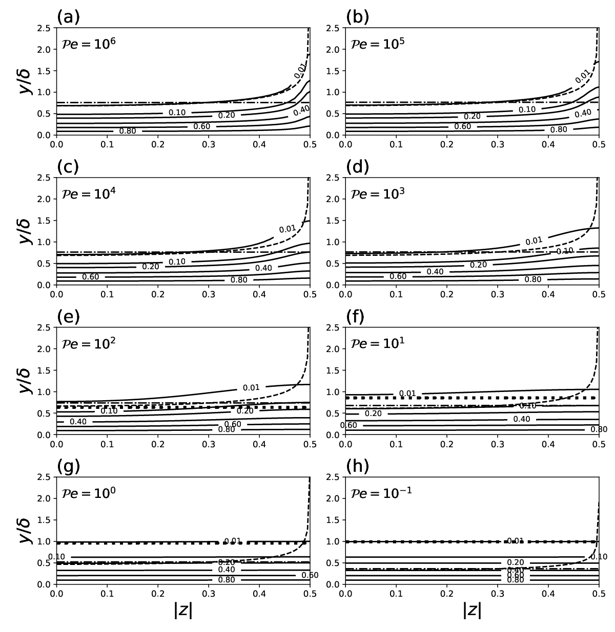
For (figures 4a–e), the two-dimensional predictions for in the thin boundary layer regime (dash-dotted lines) are in agreement with the three-dimensional numerical results in the interior of the channel . Near the side walls (), the two-dimensional predictions underestimate the numerical three-dimensional results ( contour plotted with a solid line) owing to the (basal) diffusive boundary layer at the wall. The diffusive boundary layer is better captured by the slice-wise thin boundary layer prediction (28) (dashed lines). The agreement improves as increases (see figures 4a,b), since the influence of the three-dimensional wall boundary layers, not captured by (28), reduces. At lower values of , we can see in figures 4(e,f) ( and , respectively) that the characteristic wall boundary layer thickness (in the -direction) increases inwards and is not small anymore. The thin boundary layer predictions are not valid anymore and increasingly underestimate with decreasing . As to , the thick boundary layer predictions for based on (35) (dotted lines) are in qualitative agreement. The agreement improves significantly when decreases, confirming the change of regime to the thick boundary layer regime, valid for , as shown in figures 4(g,h) where , , respectively. The dotted lines and the contour line almost overlap in figures 4(g,h). The concentration profile becomes uniform across the channel width as we predicted in §5.2.
5.5.2 Three-dimensional fluxes
To analyze the impact of the three-dimensional fluctuation flux on the total flux or Sherwood number, we plot in figure 5 , , and from (37) and (38), computed numerical using (40–42) (see table 3, appendix B, for more details). We also show the asymptotic predictions for (lines with lozenges) computed using (28).
The results indicate that the effect of the mean flux is much stronger than the effect of the fluctuation flux since for most (figure 5a) and (figure 5b) across all regimes: the thin boundary layer regime, ; the transition regime, ; and the thick boundary layer regime for . We also note that tends to reduce the flux and Sherwood number since and . The fluctuation flux, which has the strongest effect at large , is primarily due to the negative effect of the wall boundary layers that develop for both and . Close to the wall, decreases and (figure 3a), whilst increases and (figure 4a–d), thus producing a negative fluctuation flux in average. It is also interesting to note that the maximum of the fluctuation flux occurs at mid-depth in the diffusive boundary layer across all regimes. This is due to the contribution being from the product of an increasing function of , the velocity fluctuation , and a decreasing function of , the concentration fluctuations . Overall, the average fluctuation flux does not exceed more that of the mean flux for all , and , which strongly suggests that it can be neglected at leading order. In particular, vanishes in the thick boundary layer regime, confirming a posteriori our assumption to neglect when (§5.2).

5.5.3 Sherwood number

In figure 6, we plot the three-dimensional numerical results for , designated as , computed using (43) as a function of , with different open black symbols for different domain heights: (circles), (crosses) and (lozenges). For , the two-dimensional numerical results (solid lines closely following the symbols), designated as , based on (44) and neglecting are in good agreement with , for all three . In the transition region (see inset in figure 6) where the distribution for both and are inherently three-dimensional, the numerical two-dimensional results are close to the numerical three-dimensional results. We find a relative deviation, , less than for , and less than for for all . We note that for and the deviation remains less than over the whole range shown. Part of this deviation is due to numerical limitations (numerical resolution and truncation in the number of eigenpairs), particularly at large . For all , the deviation increases monotonically with increasing , in agreement with the results in figure 5, which show that the contribution of increases at large . At large , the deviation should converge to the theoretical deviation between the slice-wise asymptotic and the two-dimensional asymptotic : . Indeed we have shown in §5.1 that as , converges to the slice-wise prediction (30), whilst converges to the two-dimensional prediction, which replaces by in (30). Our numerical results appear to confirm this prediction. For in figure 6, we find as . For larger , we find that the magnitude of the deviation is smaller than for (=5) and (). Computation of additional eigenpairs for would extend these ranges to larger . Therefore, the results in figure 6 strongly suggest a posteriori that the three-dimensional flux contributes to a small portion of for all and all .
An important implication for practical applications where high accuracy is not critical is that can be neglected to solve the simpler two-dimensional problem (44), thus reducing computational burden. For a given resolution in all directions, a three-dimensional solution requires more memory for the storage of the grid by a factor of at least compared with a two-dimensional solution. For matrix-based solvers such as LAPACK (Anderson et al. 1999), computational time increases by a factor of approximately in the three-dimensional case. Therefore, though not fully optimised, the shooting method used to solve the two-dimensional case is memory efficient and could be run on portable platforms with limited memory, such as mobile phones.
At large , the slice-wise thin boundary layer prediction (30) for (dashed line in figure 6) is in agreement with . At , the deviation between them is for , for , and for . The increase of the deviation with increasing is due to the numerical limitations mentioned above: a combination of the truncation error from taking a finite number of terms in (43) and a reduced resolution since the number of grid points is fixed for all our computational domains (see also table 3, appendix B). This is a common problem when solving eigenvalue problems using finite-difference methods (Pryce 1993). The effects of truncation error and reduced resolution are noticeable at large for the results in figure 6 for (, not shown), (, not shown), (). This emphasises the importance of our asymptotic solutions providing accurate predictions in regimes where numerical results are computationally expensive and prone to numerical errors.
At small , the thick boundary layer prediction (36) (dash-dotted line) follows the numerical results as long as . As , the Sherwood number follows a different regime: , as predicted by (33) (filled blue stars). The transition between the confined regime () and the unconfined regime () can be estimated at low Péclet numbers using . We find for (circles), (crosses) and (lozenges) that the transition occurs for 0.6, 0.04 and , respectively, which agrees with the results shown in figure 6. In the confined regime we also find that increases approximately linearly with at a sufficiently small and fixed , as predicted by the asymptotic scaling in (34).
In the transition region for (inset in figure 6) the maximum error between the asymptotic theoretical predictions and the three-dimensional numerical calculations, found at the intersection of (dashed line) and (dash-dotted line), is always less than approximately . Since we expect the transition to be smooth, at least for Stokes flow, we propose a Padé approximant combining both asymptotic limits:
| (45) |
(red dotted line in the inset), where the two numerical coefficients have been computed using a least-squares fit. The approximant agrees with the three-dimensional numerical results to better than % for , and to better than 7% for . Therefore, in practical applications requiring slightly less accuracy, the asymptotic predictions and the combined fit (45) can provide instantaneous quantitative predictions of the Sherwood number as long as . The asymptotic scaling (34) also provides qualitative predictions of in the confined regime .
6 Channels with a truncated wedge geometry
6.1 Thin boundary layer regime,
In truncated wedges (figure 2), for we can use the Lévêque approximation in the diffusive boundary layer, similar to parallel channels (§5.1). The shear rate depends on following (14). In this regime, the four terms in the advection–diffusion equation (18) (in cylindrical coordinates) scale such that
| (46) |
which suggests that , as found for parallel channels. The cross-channel diffusion term is negligible since or smaller. The curvature term (second term on the right hand side of (18)), not present in parallel channels, is also negligible at leading order, and of order compared with the radial diffusion term and axial advection term. We note that can be or . At leading order, (18) reduces to the slice-wise modified Lévêque problem: , where depends parametrically on , making the problem three-dimensional. This is the same equation as in parallel channels (see (26)). Hence, the slice-wise Sherwood number is
| (47) |
for . The diffusive boundary layers along the side walls, where is not negligible, are very thin. Their thickness, in the cross-channel (-) direction, is of the order . Their contribution to the flux can therefore be neglected at leading order. Similar to parallel channel, for the small deviation between our slice-wise solution (which assumes a three-dimensional velocity and use in (47)) and the two-dimensional solution (which assumes a uniform velocity and use instead) is (for ). The deviation increases slightly with the opening angle. For , and , we find: , and (with eigenpairs), respectively (see figure 4(a), appendix A).
We now consider the influence of the higher order curvature term, neglected above. We still assume , i.e. the next terms in are neglected. We also assume so that the curvature term in (18) is much larger than the cross-channel diffusion term. The advection–diffusion equation (18) becomes
| (48) |
We change the variables from to , with , which represents the ratio of and , and the similarity variable for the advection–diffusion equation at leading order. After substituting a Poincaré expansion: , we find that the next term at order (see appendix C.1 for further details), is
| (49) |
Hence, we obtain the slice-wise Sherwood number, with the first order correction ,
| (50) |
for or , and . If terms are included in in (48), we find a similar correction for with in (50) replaced by where the function must be computed numerically. We note that this expansion, at first order in , is valid only if . If or , the scaling analysis (46) shows that the cross-channel diffusion term, neglected in (48), is of the same order or larger than the curvature term. Thus, cross-channel diffusion would need to be included in (48). This is intuitively expected as the wedge approaches the parallel channel as .
6.2 Thick boundary layer regime
The terms in the governing advection–diffusion equation (18) for scale such that
| (51) |
where we used and in the diffusive boundary layer. In this regime, the boundary layer thickness is much larger than the local width of the channel: , which implies strong cross-channel diffusion (last term in (51)) compared with streamwise advection, radial diffusion and the curvature–diffusion term (first, second and third terms in (51), respectively). Thus, we need to examine the influence of two small independent parameters: a physical parameter ; and a geometrical parameter , the opening angle, which shows that the curvature term is also negligible compared with cross-channel diffusion. Therefore, similar to parallel channels (see §5.2), cross-channel diffusion dominates in (18) and we have at leading order. This implies is independent of at leading order, owing to the no-flux boundary condition at the walls.
To analyse the two-dimensional dependence of on and , we use the cross-channel averaged advection–diffusion equation (22), where is negligible compared with . Equation (22) becomes, for and ,
| (52) |
The terms in (52) scale as the first three terms in (51), which shows that different balances can arise depending on the ratio of the two small parameters and , i.e. . We examine three sub-regimes: if , sub-regime (i), the dominant balance is between streamwise advection and radial diffusion; if , sub-regime (ii), or , sub-regime (iii) the curvature term is also important and all three terms need to be taken into account at leading order to determine and eventually the Sherwood number .
(i) For , the wedge velocity is . Then, substituting and in (52) and using a two-parameter expansion: , we find at leading order (see appendix C.2 for further details), similar to (35) in parallel channels as expected intuitively. At the next order in , we find . At order , we find
| (53) |
The Sherwood number including the corrections at order , is
| (54) |
for with and . To compute higher-order corrections for , the velocity field must also be expanded at the next order in .
(ii) For , we effectively have only one small parameter . The velocity is . All three terms in (52) are important, and the resulting equation
| (55) |
is not amenable for asymptotic expansions. Thus, we compute and numerically in this sub-regime in §6.5. However, we expect that , for . Then, we intuitively expect to be a function of and at leading order, with .
(iii) For we have two small parameters: and , and . Similar to (ii), all three terms in (52) are important and
| (56) |
is not amenable for asymptotic expansions. We also compute and numerically in §6.5 in this sub-regime. Nevertheless, we can expect that , for . We also expect to be a function of and at leading order, following the results found in other regimes. We will show in §6.5 that is indeed the correct scaling, whilst the Sherwood number varies slightly from the expected scaling.
It is also worth noting that in sub-regime (iii), and , curvature effects have a direct impact on and through a curvature-rescaled Péclet number . This rescaling is due to the opening geometry of the wedge allowing the velocity to increase as . Hence, we have . The curvature-rescaled Péclet number is somewhat analogous to the Dean number, (with the characteristic pipe flow Reynolds number, the pipe diameter and a characteristic radius of curvature of the pipe flow), which accounts for secondary recirculation flows due to curvature effects in slightly bent pipe flows (Berger et al. 1983, e.g.).
In summary, the two-dimensional thick boundary layer regime exists for wedge flows provided both and . Sub-regime (i) only exists for small enough opening angle: , which is effectively possible for . Sub-regime (iii) only exists for thick enough diffusive boundary layers: , which is only possible for . If either or , the diffusive boundary layer is not thick compared with the local width of the gap and the thick boundary layer regime does not apply. Terms in the governing equation (22), which have been neglected or considered small in this regime, can become important. In §6.5, we explore using numerical calculations whether the two-dimensional thick boundary layer regime holds beyond its theoretical range of validity or whether three-dimensional effects become important.
6.3 Radial confinement,
Similar to §5.3, we study the impact of radial confinement on using the cross-channel averaged advection–diffusion equation (22) under the free-slip and no-flux top boundary condition (4d). Integrating (22) in the streamwise direction from to , we obtain
| (57) |
with the radial flux at a particular coordinate. A new term exists compared to parallel channels and (37): the second term on the left-hand side is due to curvature. Integrating again in the radial direction from to , we obtain
| (58) |
where the curvature term has been integrated by parts. Similar to §5.3, we assume that is either negligible compared to or scales in a similar fashion. We will discuss this assumption in detail in §6.5, but we note that in the thick boundary layer regime (see §6.2) we showed that . For , we must have . Hence,
| (59) |
with (and from (10)) the wedge volume flow rate and the mean channel velocity. We have neglected the weak dependence of with in the integral on the left hand side of (6.3). In the limit of small or large channel heights, we find that the radially confined Sherwood number is: for , since in the direction; for and or , since is nearly uniform in the direction at leading order for small enough opening angles; and for and , where the curvature-rescaled Péclet number appears again, as in sub-regime (iii) of the thick boundary layer regime (see §6.2).
6.4 Transition regime, or , and numerical formulations for three- and two-dimensional problems
In wedge flows, for or , or for , and in sub-regimes (ii) and (iii) of the thick boundary layer regime (see §6.2), is three-dimensional. We study the impact of three-dimensional effects on by solving (18) numerically under (4a,b,d–f) and using our three-dimensional result (10) for . Using the same method as in §5.4, homogenisation of the boundary conditions, followed by separation of variables, leads to
| (60) |
The eigenpairs and are solutions of the homogeneous eigenvalue problem
| (61) |
for all integers , , , , with boundary conditions
| (62) |
We compute in (60) using and the orthogonality of the eigenfunctions. As in parallel channels, we solve a second-order finite difference formulation of (61) using LAPACK (Anderson et al. 1999) (see more detail in appendix B).
For comparison, we also solve a two-dimensional formulation of this problem based on the cross-channel averaged equation (22), neglecting the three-dimensional flux :
| (63) |
for , , under (4a,b,d). Homogenisation of the boundary conditions leads to a one-dimensional eigenvalue problem, which we solve using a shooting method (Berry and De Prima 1952) to obtain and a two-dimensional . This simpler two-dimensional formulation of the transport problem in wedges allows us to assess a posteriori the error on when neglecting the three-dimensional flux .
6.5 Results in truncated wedges
In this section, we compare our asymptotic predictions for and in the wedge geometry with three- and two-dimensional numerical calculations of the advection–diffusion equation. Similar to §5.5, the aim here is to assess whether three-dimensional effects related to the corners or due to confinement have a strong impact on and in the different regimes identified previously. We study the influence of , , which controls the importance of curvature effects, not present in parallel channels, and lateral and radial confinement effects. We also analyze the relative magnitude of the three-dimensional fluctuation flux and whether it can be neglected in (22).
6.5.1 Concentration field
In figure 7, we show contour plots in polar coordinates of at the end of the area of release, , for various Péclet numbers: from (figure 7a) to (7h). For conciseness, we only show results for . At smaller angles , the concentration converges towards the parallel geometry, while curvature effects are increasingly important at larger . Solid lines show the three-dimensional numerical results computed using (60–62). We normalise the -axis by , computed as with . As can be seen in figure 7, this leads to a distortion of the region being viewed, with lower cases having a much greater range of . The dashed lines, shown in figures 7(a–d) where , are plotted using the thin boundary layer predictions (28) (substituting by ) with the first-order curvature correction (49), which used , from (14), but assumed no cross-channel diffusion. The dash-dotted lines are plotted using (28) and (49) assuming a two-dimensional velocity profile, i.e. replacing by . These two predictions correspond to or . The dotted lines, shown in figures 7(d–h) where , are plotted using (35) (substituting by ) for with the first-order curvature correction (53) in . These lines show the asymptotic predictions in the thick boundary layer regime, sub-regime (i), for or .

Similar to the parallel geometry, for (figures 7a–c) the two-dimensional thin boundary layer predictions (dash-dotted lines) are in reasonable agreement (within deviation) with the three-dimensional numerical results in the interior of the channel . The diffusive boundary layer is better captured by the slice-wise thin boundary layer predictions (dashed lines) at large since the influence of the wall boundary layer reduces (see figures 7a,b) for ). The main distinction between this and the parallel geometry is that the transition between the thin and thick boundary layer regimes can occur at lower in the wedge and over a wider range: approximately (see figures 7d–h). The transition occurred for in parallel channels (see figure 4). This is due to curvature effects when is not very small, such as here with . Then, as decreases, the concentration contours flatten owing to cross-channel diffusion, which becomes the dominant effect at low . We can also notice that the thick boundary layer prediction for in sub-regime (i) (dotted line in figures 7d–h) only has approximate agreement with the numerical results (see concentration contour ) in a sub-range of the transition: for . At lower , the prediction in sub-regime (i) consistently underestimates , with increasing deviation from the numerical results as decreases. This is due to the fact that is too large for sub-regime (i) because this sub-regime is theoretically valid for (§6.2). Nevertheless, the contour plots reveal that the asymptotic results from sub-regime (i) still provide qualitative prediction at angles an order of magnitude larger than its theoretical range of validity. For , sub-regimes (ii) and (iii) are valid for and , as shown in table 1. In these two sub-regimes, curvature effects become more important, enhancing radial diffusion and leading to thicker boundary layers, comparatively with sub-regime (i) or parallel channels.
| Thin boundary layer regime | ||||
|---|---|---|---|---|
| Thick boundary layer regime | ||||
| Sub-regime (i) | – | – | – | |
| Sub-regime (ii) | ||||
| Sub-regime (iii) | ||||
| (radial confinement) | ||||
| Confinement regime | (i) | (iii) | (iii) | (iii) |
| † | † | † | ||
| Thin boundary layer regime | ||||
| Thick boundary layer regime | ||||
| Sub-regime (i) | – | – | – | |
| Sub-regime (ii) | – | – | – | |
| Sub-regime (iii) | – | – | – | |
| (radial confinement) | ||||
| Confinement sub-regime | (iii) | (iii) | (iii) |
6.5.2 Three-dimensional fluxes
To analyze the impact of the three-dimensional fluctuation flux on the total flux or Sherwood number, we plot in figure 8 and from (6.3), computed numerically using (60–62) for (symbols and solid line), (symbols and dotted line), (symbols and dashed line), (symbols and dash-dotted line) and (symbols and long-dashed line) (see table 3, appendix B, for more details). We show the asymptotic predictions for computed numerically using (28) (substituting by ) and the first-order curvature correction (49). They correspond to the horizontal lines plotted with a line style matching the numerical results for each .

Figure 8 shows that in the thick boundary layer regime (low ), the negative contribution of the total fluctuation flux vanishes for all . For , larger values of lead to a faster increase in the contribution of , thus extending the range of the transition between thin and thick boundary layer regimes for . In the thin boundary layer regime (large ), reduces the contribution from that evaluated just on the mean flux by between approximately () and (). The numerical calculations (symbols) converge asymptotically towards the predictions in the thin boundary layer regime at large . The thin boundary layer predictions capture the increasing trend in the contribution of with increasing . For , the results are similar to those obtained in parallel channels (figure 5b). This suggests that a two-dimensional description of the flux in wedges is also appropriate at leading order for the full range of Péclet numbers studied, provided . At this stage, it is uncertain whether a two-dimensional description remains accurate at large and for or whether three-dimensional effects must be included. We discuss this further below.
6.5.3 Sherwood number

Figure 9 shows computed from the three-dimensional numerical calculation of (60–62) versus , for , and for: (blue circles), (orange crosses), (green lozenges), (red stars), (violet squares), (brown hexagons), (pink pentagons). The solid lines closely following the symbols correspond to the two-dimensional numerical results based on (63), neglecting the three-dimensional flux (see table 3, appendix B, for details about the numerical computations). For , the two-dimensional numerical results are mostly in agreement with the three-dimensional numerical results. For , we find that the deviation between the two-dimensional and the three-dimensional results is within less than for , and for . For , the deviation is within less than for , and for . The deviation for intermediate are within the same bounds. The increased deviation observed for and (brown and pink curves, inset of figure 9) is due to a combination of truncation error and reduced resolution in the calculation of , which is performed using different methods between the two-dimensional and three-dimensional numerical calculations. In general, we find that increasing the resolution and the number of eigenpairs for the calculation of reduces the deviation at large and for up to (see appendix B.3, figure 4(b)). This also improves the agreement between the numerical results and the slice-wise thin boundary layer predictions (50) at large (dash-dotted lines using matching colours for each , inset only). We can also notice that the curves do not collapse at large . This is due to the fact that depends on (see (50)).
The results in figure 9 clearly demonstrate that for applications not requiring a high accuracy for , the three-dimensional fluctuation flux can be neglected and the two-dimensional formulation (63) can be used for all and up to at least . As mentioned in §5.5, the two-dimensional formulation significantly reduces computational burden whilst preserving reasonable accuracy. In addition, our slice-wise thin boundary layer predictions (50) provide fast and accurate complementary estimates of in the computationally challenging regime at and for all .
As decreases, a more complex behaviour emerges due to the increased effect of curvature for non-negligible opening angles. For (blue symbols and curves in figure 9), curvature effects are negligible and, as long as (), the two-dimensional thick boundary layer predictions (54), sub-regime (i), , or (dashed lines using matching colours for each in main graph), agree with the numerical computations in the range predicted in table 1. Then, as increases, increases at fixed , departing from this prediction (see all colours other than blue). This is due to the fact that increases and sub-regime (i) is not valid any more. As shown in table 1, for sub-regime (i) disappears and the diffusive boundary layer can be in sub-regimes (ii) or (iii) of the thick boundary layer regime, where the curvature term in the advection–diffusion equation (52) becomes non-negligible and no asymptotic predictions exist for in sub-regimes (ii) and (iii). Table 1 presents the range of where sub-regimes (ii) and (iii) are valid, provided . For , the results shown in violet, brown and pink cannot be considered in the thick boundary layer regime since (see scaling analysis in §6.2).
Then, if , all the terms in the governing advection–diffusion equation (18) are important, making the problem even more three-dimensional and requiring full numerical calculation of (18). As can be seen in figure 9, an increase in leads to an increase in , which appears to tend towards a plateau, reducing its dependence with .
At very low , radial confinement becomes important and the curves follow another regime: (see (59)) similar to parallel channels (see figure 6). The at which the the radially confined regime occurs depends on the regime that the boundary layer would be without confinement effect. The corresponding transitional and the associated regime are indicated in the rows “” and “Confinement regime” in table 1. The predictions for the transitional (black stars in figure 9) agree with the numerical results. For , since the thick boundary layer regime is not theoretically valid, as discussed previously, the predictions given in table 1 assume that the diffusive boundary layer is in sub-regime (iii) of the thick boundary layer regime. As shown in figure 9, the estimated transitional are still accurate even for , at least up to (see black stars for the violet squares, brown hexagons and pink pentagons). We note that the locus of the confinement transition is not a simple curve. This is partly due to the fact that the confinement transition occurs in different sub-regimes, but also that for , 1 and the transition does not occur in an asymptotic regime, as stated in table 1.

Sub-regime (iii) of the thick boundary layer regime occurs only at very low Péclet numbers: . As seen in table 1, this regime may only appear in figure 9 for a very limited range of and for and 0.3 only, as radial confinement effects also become important at similar . In sub-regime (iii), we noted in §6.2 the importance of a curvature-rescaled Péclet numbers since . In general, we must have when for sub-regime (iii) to exist without being affected by radial confinement effects. To show sub-regime (iii) more clearly, we plot in figure 10(a) for various as a function of , effectively ranging . All the results shown in figure 10(a) and (b) were computed numerically using the two-dimensional formulation (63), for and . We decided to use the two-dimensional formulation, instead of the exact three-dimensional formulation, due to computational difficulties in reaching sufficiently low . We expect the results to remain accurate since, as we have shown previously, the error made using the two-dimensional formulation remains small, particularly at low and low . We can see that for , the predicted transition for sub-regime (iii), all the curves collapse and , as suggested by our scaling analysis in §6.2.
In contrast with , we find that (figure 10(b)) does not follow the intuitive scaling . Instead, the collapse of the curves suggests a different trend in sub-regime (iii): , or equivalently . However, we have not been able to confirm this result analytically. We find that this empirical collapse occurs for , as long as radial confinement effects are not important. Radial confinement effects occur when , or , as shown by the radical change of regime at lower in figure 10(b).
The weaker dependence of on in the limit of vanishing and , assuming no radial confinement effects, shows that multiple effects become important in addition to the streamwise advection–radial diffusion balance. This has been observed both in the asymptotic sub-regime (iii) in figure 10(b) and the regime in figure 9. Curvature effects become important and the velocity field increases such that due to the opening of the wedge channel. These combined effects are the cause of the observed plateau in the Sherwood number in figure 9, as and , which implies an enhanced mass transfer compared with parallel-wall channels. This is intuitively expected as lateral confinement effects vanish with increasing opening angle.
7 Discussion and implications for practical applications
As mentioned in §1, this study applies to the removal of contaminant trapped in sub-surface features such as gaps, cracks or folds. We assumed that the area of release is constant and flat, and does not impact the velocity field. In practice, the contaminant may take the shape of a droplet which can perturb the flow in various ways: for instance through changes in the height of the channel, particularly when , causing a change in velocity and modifying , thereby affecting the mass transfer. We also assumed that the scalar released is passive. It is likely that this assumption is justified for slowly dissolving or low solubility substances such as found in many cleaning and decontamination scenarios. Otherwise, changes to the density or viscosity of the cleaning agent need to be accounted for. For example, if transport of the scalar leads to a significant change in fluid density, buoyancy effects should be considered. Significant changes of the fluid viscosity with tracer concentration could change the shear profile in ways which could affect the Sherwood number. This may be of particular importance for materials such as highly soluble liquids with high viscosity.
Another potential limitation of this study is the geometrical simplification of the bottom of the channel, particularly in the case of mass transfer. A dissolving droplet or solid at the bottom of the channel may not have a flat surface, as assumed in the parallel-wall geometry, or a convex circular surface, as assumed in the truncated wedge geometry; or its shape may be affected by the dissolution process itself. We did not consider this level of detail in order to obtain simple analytical expressions and deduce key physical insight, which might have been lost in a full numerical treatment.
Applications with slow changes in time of the source concentration can also exploit our results under the assumption of a quasi-steady diffusive boundary layer. The concentration profile and mass transfer in the diffusive boundary layer can be considered to adjust instantaneously to the changes in the source concentration (Landel et al. 2016, see).
The key and most intuitive implication of our findings to decontamination and cleaning applications is that increasing the Péclet number improves the flux, which then allows for better neutralisation of the substance through reactions in the bulk. We find that increasing the width of the channel has the strongest impact on increasing . Indeed, we have since the characteristic channel velocity increases quadratically with . However, changes of the channel width are only possible through alterations of the material. Such techniques may not be favoured due to their destructive potential for substrates, but could be considered at the designer stage for some applications.
The main physical parameter generally controlled in cleaning and decontamination applications, and which can increase in a less destructive way, is the flow velocity since . The local velocity in the channel is controlled by pressure forces, gravity, viscosity and capillary forces. Therefore, reducing the viscosity of the cleansing flow, through through the formulation or an increase of temperature for instance, or increasing the pressure gradient, could lead to increasing . Depending on the geometry and the regime, different gains in the flux can be obtained. For example, in the case of parallel channels, the highest gain is obtained when the flow is confined vertically: doubling the speed will also double the Sherwood number and thus the overall flux. If the boundary layer is unconfined vertically but confined in the lateral direction (thick boundary layer regime), doubling yields an increase by in the flux. In the thin boundary layer regime, where the boundary layer is unconfined, doubling yields an increase of only in the flux. However, these results are valid provided that the boundary layer does not change regime. As increases, decreases, reducing confinement effects and potentially leading to a change in regime. Consequently, while there are still gains in the flux, the gains may be smaller. Increasing inside sub-surface channels can be challenging. Most decontamination and cleaning techniques involve surface washing which has a limited effect on the velocity in sub-surface features, which may be driven purely by gravitational draining.
Mass transfer from the area of release through a diffusive boundary layer is a first but key step towards complete removal in the context of cleaning and decontamination. For very long channels, scalar transport beyond the area of release, i.e. for , becomes a Taylor–Aris problem (Taylor 1953; Aris 1956) with non-uniform inlet scalar profile (see figures 4 and 7 for concentration profiles at the downstream end of the area of release). Giona et al. 2009 study the dispersion of a scalar transported in laminar channel flows with various smooth and non-smooth cross-sectional geometries. They consider the case of impulse feeding with no-flux boundary condition on all the channel walls. Their results describe the evolution of the scalar distribution beyond the area of release but at a finite distance, thus complementing the works of Taylor 1953 and Aris 1956 who looked at the far field distribution. Similar to our , their effective Péclet number compares the axial convective time scale to the transverse or cross channel diffusive time scale. In the limit of vanishing effective Péclet number they recover the Taylor–Aris regime, whilst for effective Péclet numbers of more than 10 they find an advection dominated dispersion regime which is characterised by wall boundary layers with slow advective transport. Their advection-dominated dispersion regime has parallels with our thick boundary layer regime, thus making the Taylor–Aris regime analogous with our thick boundary layer regime.
The existence of the advection dominated dispersion regime has practical implications for decontamination problems. The scalar can be trapped in boundary layers close to the walls (Adrover et al. 2009). This can increase its dwelling time in the channel and could potentially enable ingress into absorbing channel walls, thus, dispersing contaminants further.
Our results are also relevant to turbulent flows, provided the diffusive boundary layer is thinner than the viscous sub-layer of the turbulent wall boundary layer if the flow. In the case of shallow cracks and gaps on a substrate, or for rough substrates, the thin film flow washing the surface can be turbulent above these features. In general the viscous sub-layer develops faster than the diffusive boundary layer, due to the high Schmidt numbers involved in typical cleaning and decontamination problems, of the order of to .
8 Summary and conclusion
We have studied in this paper the convective transport of a passive scalar released at the base of generic rectangular channels with parallel walls and channels with a truncated wedge cross-section with angled walls. Our main objective was to predict the flux or Sherwood number as a function of the flow, scalar properties, and the geometry. Due to the lateral and vertical or radial confinement, the resulting diffusive boundary layer for the scalar is three-dimensional. This makes the problem too complex to solve analytically in the general case. Using a combination of asymptotic analysis and numerical calculations, we have found that different regimes exist for depending mainly on the ratio of the diffusive boundary layer thickness and the gap width . We have also shown that is a function of a characteristic Péclet number, , and the opening angle for wedges, depending on the regime. An important and unexpected conclusion is that in all the regimes identified, two-dimensional approximate models can provide accurate quantitative predictions for across all the parameters and geometries explored, despite the problem begin fundamentally three-dimensional. We summarize in table 2 the different predictions for , and for each regime and channel geometry. The main remarks of our study are:
| Channel geometry | Parameter | |||
|---|---|---|---|---|
| and regime | range | |||
| Parallel wall | ||||
| Thin boundary layer regime | ||||
| (slice-wise Lévêque regime) | ||||
| (confined) | ||||
| Thick boundary layer regime | ||||
| (confined) | (33) | |||
| Transition | ||||
| (4) | ||||
| Truncated wedge | ||||
| Thin boundary layer regime | ||||
| (slice-wise Lévêque regime) | ||||
| (confined) | ||||
| Thick boundary layer regime | ||||
| , sub-regime (i) | ||||
| (confined) | ||||
| , sub-regime (ii) | ||||
| (confined) | ||||
| , sub-regime (iii) | † | |||
| (confined) | ||||
| Transition | ||||
| (10) | – |
- •
In the thin boundary layer regime, , both geometries follow the classical Lévêque regime with . Since , the influence of the geometry, whether curved or not, and the effect of lateral confinement are negligible, except for where . We find that the effect of the diffusive boundary layers due to the no-flux side walls is small, decreasing with increasing Péclet number, which explains why two-dimensional approximate models provide accurate results in this regime.
- •
In the thick boundary layer limit, , cross-channel diffusion is dominant and the concentration is uniform across the channel. For parallel wall channels, is asymptotically constant with distance from the base of the channel. The resulting Sherwood number follows . In parallel channels, we find a smooth transition between the thick and thin boundary layer regimes at intermediate Péclet numbers, that is empirically described by the Padé approximant . In contrast, the Sherwood number in the truncated wedge geometry follows a more complex behaviour across the transition regime and the thick boundary layer regime, depending on the opening angle and . As increases at a fixed , we find that has a linear dependence with increasing . For , we find that the dependence of with decreases. This is due to curvature effects. As increases, the influence of the no-flux boundary condition at the side walls is lessened, which tends to enhance curvature-induced diffusion.
- •
We also found another effect of increasing the opening angle in which the velocity field is less constrained by the side walls and increases quadratically with and . Thick boundary layers then experience an increasing velocity with distance from the area of release: . In this regime, sub-regime (iii), we showed that the diffusive boundary layer thickness scales with a curvature-rescaled Péclet number , such that in the limit , provided so that the flow is not constrained radially. However, we find that the Sherwood number does not follow the intuitive scaling , but instead appears to follow the empirical scaling . This enhanced flux is due to increased diffusion from curvature effect. The curvature term in the cross-channel averaged advection–diffusion equation in cylindrical coordinates is a leading order term in this limit. Therefore, to predict accurately its effect on the resulting mass transfer, numerical computation is necessary.
- •
We have also shown that it is not necessary to solve the full three-dimensional advection–diffusion equation to obtain an accurate estimate of . The results for predicted by solutions to the simplified two-dimensional cross-channel averaged advection–diffusion equations (44) and (63), for parallel wall channels and truncated wedges respectively, agree with the full three-dimensional numerical solution to better than for for all curves calculated. We have also shown that this can be extended towards larger by improving the numerical resolution. These simplified equations neglect the contribution to the overall flux of the three-dimensional fluctuation flux , which can be responsible for up to of the total streamwise flux at some height for large and , but is negligible for low as shown by our asymptotic analysis and numerical results. It is therefore somewhat surprising that the significant non-zero contribution from , which varies with the height above the base, leads to only a small net contribution to the three-dimensional Sherwood number after integration over the depth of the flow. Nevertheless, our findings reveal that the net effect of this -varying contribution, integrated over the depth of the flow, leads to only a small deviation on the two-dimensional Sherwood number for all Péclet numbers and opening angles. The asymptotic analysis shows that in the limit of large a two-dimensional computation over-predicts the Sherwood number by only for channels with parallel walls and by less than for truncated wedges with . Therefore, the two-dimensional equations (44) (parallel channels) and (63) (wedges) will be useful to many applications where improving computational speed is critical.
- •
In addition, we have demonstrated that vertical (parallel channels) and radial (wedges) confinement lead to when for all the geometries studied and at any Péclet numbers. Effectively, vertical or radial confinement has the strongest impact on reducing the flux. This is due to significant reduction in the gradient of the concentration field normal to the area of release. This is an important finding for applications optimising convective fluxes in narrow spaces.
The two geometries studied provide insight as to the impact of having other opening channel geometries such as convex or concave side walls of complex profiles. The impact occurs mainly in the thick boundary layer regime where the velocity field varies depending on lateral confinement. From scaling analysis, we find that , for . As the channel width increases, the resulting increases owing to a combination of enhanced streamwise advection and enhanced diffusion through curvature effects. An accurate dependence of with flow and geometrical properties can be computed numerically using the simplified two-dimensional equations (44) or (63). Nevertheless, we note that the dependence with the Péclet number will be of the form , where the exponent is a function of , provided increases with . We predict that this result is valid for all and . For , our previous result should hold, being valid for any geometry.
The low dependence of the average flux on cross-channel variations found for all geometries and across all Péclet numbers is an important result. Specifically, by neglecting three-dimensional effects, the broad range of advanced analytical techniques for two-dimensional problems can be exploited to obtain further result. For instance, conformal mapping and potential flow techniques could explore how the Sherwood number depends on more complex geometry and flow profile in the or plane (Bazant 2004; Choi et al. 2005). Our results strongly suggest that small variations to the geometry and flow profile in the cross-sectional plane, beyond the geometries studied here, are unlikely to be important. However, we leave the case of more complex cross-sectional variations for future studies.
Appendix A Additional material related to the flow field
Figure 3(a) shows the dependence of the cross-channel averaged bottom shear rate with for parallel channels. We find that rapidly approaches an asymptotic value of approximately 3.26 for . Figure 3(b) presents similar results as in figure 3(a) for truncated wedges of various angles . The mean shear rate increases with increasing . The channel height required for to reach an asymptotic plateau increases with .
In figure 4(a) we show the dependence of the negative deviation with and . This corresponds to the deviation between the slice-wise and the two-dimensional solution of in the thin boundary layer regime, see equation (30) for parallel-wall channels and (47) for truncated wedges. The numerical results are computed using eigenpairs for based on (14). For , the deviation appears to reach an asymptotic plateau for . We see that for the magnitude of the deviation approaches the value for channels with parallel walls, approximately . At , the deviation remains small, slightly larger than for and .
Appendix B Numerical computations
B.1 Verification of our numerical schemes
We verified our numerical schemes for the computation of the three-dimensional and two-dimensional problems (see §5.4 and §6.4) by recovering the well-known Lévêque solutions for heat transfer in the thin boundary layer limit, which solves the scalar transport equation
| (64) |
for and with boundary conditions
| (65) |
The solution for this problem is given in classical texts such as Bejan 2013. In appropriate dimensionless form it is
| (66) |
where is the Sherwood number (defined as ) and the appropriate Péclet number () (Bejan 2013).
The two-dimensional numerical scheme used in this paper solves (44) with boundary conditions (4a,b,d), on a finite domain with . Since the governing equation (64) with boundary conditions (65) is defined for an unconfined flow (), we expect the numerical solution to diverge from the analytical solution for small as the boundary layer assumption made in deriving (64) is no longer valid (see also (Bejan 2013)) when the boundary layer thickness appropaches .
The three-dimensional numerical scheme used in this paper solves (16) with boundary conditions (4a,b,d-f). It is expected to recover (66) if . Note that the velocity field in this model problem is inconsistent with the lateral boundary conditions at in (3) and does not depend on . Therefore, the three-dimensional code also solves the two-dimensional problem (66) provided, as for the two-dimensional case, that the boundary layer thickness is much smaller than the channel height.
Figure 1 compares the three-dimensional numerical solutions for two different domain heights and resolutions (crosses: , (grey) and (black); circles: , (grey) and (black)) against (66). In figure 1(a) the numerical solutions are plotted together with the analytical solution (66) (solid line). The error between the numerical and the analytical solution is plotted in figure 1(b). A minimum error exists for both : for , the minimum is at ; for at . The boundary layer thickness scales as (Bejan 2013). Therefore, corresponds to and to , thus, the effect of vertical confinement on the boundary layer becomes non-negligible as , as anticipated above.
Figure 1(b) shows that for () and the error is less than for about 2.5 orders of magnitude in for the lower resolution calculations and about 4.5 orders of magnitude for the higher resolution calculations. The error increases again with increasing as the boundary layer thickness decreases and approaches the numerical resolution. For example, for resolved as (black crosses), for an error of . This corresponds to a boundary layer thickness of about , which approaches the grid size (0.0375). At this resolution, the boundary layer can only be resolved with reduced accuracy for .


We proceed analogously for the validation of the two-dimensional scheme. The results are compared directly in figure 2(a). Figure 2(b) shows the relative error. Similar to before, circles indicate solutions with and crosses with . Since we were able to choose a large resolution on a one-dimensional grid (, consistent with other computations in this paper), we only investigate one resolution. Since the shooting method computes the eigenvalues serially (Berry and De Prima 1952) and the computational effort increases for larger eigenvalues, the truncation of the series is required nevertheless. Consistent with the solutions obtained from the three-dimensional code, we find a minimum value of at which the two solutions agree, which is consistent between both codes since both codes solve effectively the same problem. As can be seen, an excellent agreement, to within (), between both solutions is obtained for both channel heights for approximately four orders of magnitude. Computation of additional eigenpairs will extend the agreement between both solutions towards smaller until the resolution limit is reached.
We note that our code verification spans multiple orders of magnitude in and therefore in . Any computation spanning such a range of values is highly challenging and expensive and is eventually limited by numerical resolution. This is one of the reasons why we supplement the numerical solutions with asymptotic solutions throughout this paper.
B.2 Numerical details
Table 3 provides details about the numerical computations presented in this study. The numerical calculations of for parallel channels (4) and for wedges (10) were affected by numerical overflows at small and large , even with 128 bit floating point precision. As an error criterion we used that in the interior of the channel (, analogous for wedges) the relative error of the flow field (defined as the difference to a computation made with 1.5 times as many eigenpairs) should be less than . For rectangular channels, velocity fields were computed with at least 5000 eigenpairs and for wedge-shaped channels the velocity fields were computed with at least 2000 eigenpairs.
Semi-infinite domains (figures 4, 5, 7, 8 and 10) were approximated by solving the flow field in a channel of sufficient height (designated ) to ensure the flow field is independent with height. The height of the domain for solving the advection–diffusion problem (designated ) was then chosen such that . We note that when , the channel height is simply designated as .
B.3 Effect of truncation error
Figure 4(b) reproduces results from figure 9, for and (solid lines and black symbols), for which we noted a larger deviation from the asymptotic prediction (50) (dash-dotted lines) for . Here the results are supplemented by three-dimensional (open symbols) and two-dimensional (dotted lines) computations at the same but with a reduced domain height for the advection–diffusion problem: from (figure 9) to (figure 4(b)) (). The numerical results now agree with the asymptotic prediction (50) for an extended range: up to . This is due to the increased resolution obtained when reducing the domain height, since the number of grid points is maintained fixed in all our computational domains (see table 3, appendix B). The drawback of reducing is that the transition to the radially confined regime occurs at higher values of .

| Figure | Resolution | EP | Notes | |||||
| or | or | |||||||
| 4(a) | 400 | 40 | 0.1 | - | 30 | 16000 | 3D LP | |
| 4(b) | 400 | 40 | 0.2 | - | 30 | 16000 | 3D LP | |
| 4(c,d) | 400 | 40 | 1 | - | 30 | 16000 | 3D LP | |
| 4(e,f) | 400 | 40 | 5 | - | 30 | 16000 | 3D LP | |
| 4(g) | 400 | 40 | 15 | - | 30 | 16000 | 3D LP | |
| 4(h) | 400 | 40 | 5 | - | 30 | 16000 | 3D LP | |
| 5 | 400 | 40 | 0.1 | - | 30 | 16000 | 3D LP | |
| 5 | 400 | 40 | 0.2 | - | 30 | 16000 | 3D LP | |
| 5 | 400 | 40 | 1 | - | 30 | 16000 | 3D LP | |
| 5 | 400 | 40 | 5 | - | 30 | 16000 | 3D LP | |
| 5 | 400 | 40 | 15 | - | 30 | 16000 | 3D LP | |
| 5 | 400 | 40 | 5 | - | 30 | 16000 | 3D LP | |
| 6 | – | 400 | 40 | 1.25,5,15 | - | 1.25,5,15 | 16000 | 3D LP |
| 6 | – | 25000 | - | 15 | - | 15 | 5000 | 2D SM |
| 7(a,b) | , | 400 | 40 | 1 | 0.3 | 200 | 16000 | 3D LP |
| 7(c) | 400 | 40 | 2 | 0.3 | 200 | 16000 | 3D LP | |
| 7(d,e) | , | 400 | 40 | 10 | 0.3 | 200 | 16000 | 3D LP |
| 7(f,g,h) | , , | 400 | 40 | 100 | 0.3 | 200 | 16000 | 3D LP |
| 8 | 400 | 40 | 0.1 | 0.1- | 200 | 16000 | 3D LP | |
| 8 | 400 | 40 | 1 | 0.1– | 200 | 16000 | 3D LP | |
| 8 | , , | 400 | 40 | 2 | 0.1– | 200 | 16000 | 3D LP |
| 8 | , | 400 | 40 | 10 | 0.1– | 200 | 16000 | 3D LP |
| 8 | , , | 400 | 40 | 100 | 0.1– | 200 | 16000 | 3D LP |
| 9 | – | 400 | 40 | 15 | 0.01- | 15 | 16000 | 3D LP |
| 9 | – | 25000 | - | 15 | 0.01- | 15 | 5000 | 2D SM |
| 10 | all shown | 25000 | - | 1000 | 0.01 - /2 | 1000 | 5000 | 2D SM |
| 4(b) | – | 12500 | - | 1 | 1, | 15 | 3000 | 2D SM |
| 4(b) | – | 400 | 40 | 1 | 1, | 15 | 16000 | 3D LP |
| 4(b) | – | 25000 | - | 15 | 1, | 15 | 5000 | 2D SM |
| 4(b) | – | 400 | 40 | 15 | 1, | 15 | 16000 | 3D LP |
Appendix C First-order correction in channels with a truncated wedge geometry
C.1 Thin boundary layer regime
In equation (48) we change the variables from to , with , which represents the ratio of and , and the similarity variable for the advection–diffusion equation at leading order. We obtain
| (67) |
Substituting a Poincaré expansion: , we find at order
| (68) |
which, as expected, leads to our modified Lévêque solution (28) (substituting by and with following (14)) and the flux (47). For , we find
| (69) |
The boundary conditions for (68) and (69) are
| (70) |
The next term, at order , is
| (71) |
C.2 Thick boundary layer regime, sub-regime (i)
[1-8] Substituting and and using , (52) becomes, at leading order,
| (72) |
with , and . Using a two-parameter expansion: , we find at leading order , similar to (35) in parallel channels as expected intuitively, and which satisfies the boundary conditions and . At the next order in ,
| (73) |
The solution is
| (74) |
with the imaginary error function, and a constant of order , which we determine below. The solution satisfies the boundary conditions and . Similarly, at order , satisfies
| (75) |
The solution is
| (53) |
which satisfies the boundary conditions and . We can now compute the Sherwood number including the corrections at order ,
| (76) |
As , we must recover the result (36) in parallel channels. Hence, and .
References
- Zhang et al. (1996) W. Zhang, H. A. Stone, J. D. Sherwood, Mass transfer at a microelectrode in channel flow, The Journal of Physical Chemistry 100 (1996) 9462–9464.
- Gervais and Jensen (2006) T. Gervais, K. F. Jensen, Mass transport and surface reactions in microfluidic systems, Chemical Engineering Science 61 (2006) 1102 – 1121.
- Kirtland et al. (2009) J. D. Kirtland, C. R. Siegel, A. D. Stroock, Interfacial mass transport in steady three-dimensional flows in microchannels, New Journal of Physics 11 (2009). doi:10.1088/1367-2630/11/7/075028.
- Vijayendran et al. (2003) R. A. Vijayendran, K. M. Motsegood, D. J. Beebe, D. E. Leckband, Evaluation of a three-dimensional micromixer in a surface-based biosensor, Langmuir 19 (2003) 1824–1828.
- Squires et al. (2008) T. M. Squires, R. J. Messinger, S. R. Manalis, Making it stick: convection, reaction and diffusion in surface-based biosensors, Nature Biotechnology 26 (2008) 417–426.
- Hansen et al. (2012) R. Hansen, H. Bruus, T. H. Callisen, O. Hassager, Transient convection, diffusion, and adsorption in surface-based biosensors, Langmuir 28 (2012) 7557–7563.
- Dejam (2019) M. Dejam, Hydrodynamic dispersion due to a variety of flow velocity profiles in a porous-walled microfluidic channel, International Journal of Heat and Mass Transfer 136 (2019) 87–98. URL: http://www.sciencedirect.com/science/article/pii/S0017931019302716. doi:https://doi.org/10.1016/j.ijheatmasstransfer.2019.02.081.
- Kou and Dejam (2019) Z. Kou, M. Dejam, Dispersion due to combined pressure-driven and electro-osmotic flows in a channel surrounded by a permeable porous medium, Physics of Fluids 31 (2019) 056603. doi:10.1063/1.5092199.
- Jönsson and Mathiasson (2000) J. A. Jönsson, L. Mathiasson, Membrane-based techniques for sample enrichment, Journal of Chromatography A 902 (2000) 205–225. doi:10.1016/S0021-9673(00)00922-5.
- Marczak et al. (2006) M. Marczak, L. Wolska, W. Chrzanowski, J. Namieśnik, Microanalysis of volatile organic compounds (VOCs) in water samples – Methods and instruments, Microchimica Acta 155 (2006) 331–348. URL: https://doi.org/10.1007/s00604-006-0630-x. doi:10.1007/s00604-006-0630-x.
- Kamholz et al. (1999) A. E. Kamholz, B. H. Weigl, B. A. Finlayson, P. Yager, Quantitative analysis of molecular interaction in a microfluidic channel: the T-sensor, Analen der Chemie 71 (1999) 5340–5347.
- Ismagilov et al. (2000) R. F. Ismagilov, A. D. Stroock, P. J. A. Kenis, G. Whitesides, H. A. Stone, Experimental and theoretical scaling laws for transverse diffusive broadening in two-phase laminar flows in microchannels, Applied Physics Letters 76 (2000) 2376–2378.
- Kamholz and Yager (2001) A. E. Kamholz, P. Yager, Theoretical analysis of molecular diffusion in pressure driven laminar flow in microfluidic channels, Biophysical Journal 80 (2001) 155–160.
- Kamholz and Yager (2002) A. E. Kamholz, P. Yager, Molecular diffusive scaling laws in pressure-driven microfluidic channels: deviation from one-dimensional einstein approximations, Sensors and Actuators B 82 (2002) 117–121.
- Stone et al. (2004) H. A. Stone, A. D. Stroock, A. Ajdari, Engineering flows in small devices: Microfluidics toward a lab-on-a-chip, Annual Review of Fluid Mechanics 36 (2004) 381–411.
- Jiménez (2005) J. Jiménez, The growth of a mixing layer in a laminar channel, Journal of Fluid Mechanics 535 (2005) 245–254. doi:10.1017/S0022112005004994.
- Capretto et al. (2011) L. Capretto, W. Cheng, M. Hill, X. Zhang, Micromixing within microfluidic devices, in: B. Lin (Ed.), Microfluidics: Technologies and Applications, Springer, Berlin, Heidelberg, 2011, pp. 27–68. URL: https://doi.org/10.1007/128_2011_150. doi:10.1007/128_2011_150.
- Ferrigno et al. (2002) R. Ferrigno, A. D. Stroock, T. D. Clark, M. Mayer, G. M. Whitesides, Membraneless vanadium redox fuel cell using laminar flow, Journal of the American Chemical Society 124 (2002) 12930–12931.
- Cohen et al. (2005) J. L. Cohen, D. A. Westly, A. Pechenik, H. D. Abruña, Fabrication and preliminary testing of a planar membraneless microchannel fuel cell, Journal of Power Sources 139 (2005) 96–105.
- Braff et al. (2013) W. A. Braff, M. Z. Bazant, C. R. Buie, Membrane-less hydrogen bromine flow battery, Nature Communications 4 (2013).
- Porter (1972) M. C. Porter, Concentration polarization with membrane ultrafiltration, Ind. Eng. Chem. Prod. Res. Dev. 11 (1972) 234–248.
- Bowen and Jenner (1995) W. R. Bowen, F. Jenner, Theoretical descriptions of membrane filtration of colloids and fine particles: An assessment and review, Advances in Colloid and Interface Science 56 (1995) 141 – 200. URL: http://www.sciencedirect.com/science/article/pii/0001868694002322. doi:https://doi.org/10.1016/0001-8686(94)00232-2.
- Visvanathan et al. (2000) C. Visvanathan, R. Ben Aim, K. Parameshwaran, Membrane separation bioreactors for wastewater treatment, Critical Reviews in Environmental Science and Technology 30 (2000) 1–48.
- Herterich et al. (2015) J. G. Herterich, D. Vella, R. W. Field, N. P. Hankins, I. M. Griffiths, Tailoring wall permeabilities for enhanced filtration, Physics of Fluids 27 (2015) 053102.
- Bisschop and Kurlov (2013) J. Bisschop, A. Kurlov, A flow-through method for measuring the dissolution rate of alite and Portland cement clinker, Cement and Concrete Research 51 (2013) 47–56. URL: http://www.sciencedirect.com/science/article/pii/S0008884613000963. doi:10.1016/j.cemconres.2013.04.013.
- Borden and Kao (1992) R. C. Borden, C. M. Kao, Evaluation of groundwater extraction for remediation of petroleum-contaminated aquifers, Water Environ Res. 64 (1992) 28–36.
- Dejam et al. (2014) M. Dejam, H. Hassanzadeh, Z. Chen, Shear dispersion in a fracture with porous walls, Advances in Water Resources 74 (2014) 14–25. URL: http://www.sciencedirect.com/science/article/pii/S0309170814001663. doi:https://doi.org/10.1016/j.advwatres.2014.08.005.
- Kahler and Kabala (2016) D. M. Kahler, Z. J. Kabala, Acceleration of groundwater remediation by deep sweeps and vortex ejections induced by rapidly pulsed pumping, Water Resources Research 52 (2016) 3930–3940.
- Wilson (2005) D. I. Wilson, Challenges in cleaning: Recent developments and future prospects, Heat Transfer Engineering 26 (2005).
- Fryer and Asteriadou (2009) P. G. Fryer, K. Asteriadou, A prototype cleaning map: a classification of industrial cleaning processes, Trends in Food Science & Technology 20 (2009) 255–262.
- Lelieveld et al. (2014) H. L. M. Lelieveld, J. T. Holah, D. Napper, Hygiene in Food Processing: Principles and Practices, 2 ed., Woodhead Publishing, 2014.
- Pentsak et al. (2019) E. O. Pentsak, D. B. Eremin, E. G. Gordeev, V. P. Ananikov, Phantom reactivity in organic and catalytic reactions as a consequence of microscale destruction and contamination-trapping effects of magnetic stir bars, ACS Catalysis 9 (2019) 3070–3081.
- Fitch et al. (2003) J. P. Fitch, E. Raber, D. R. Imbro, Technology challenges in responding to biological or chemical attacks in the civilian sector, Science 302 (2003) 1350–1354.
- Settles (2006) G. S. Settles, Fluid mechanics and homeland security, Annual Review of Fluid Mechanics 38 (2006) 87–110.
- Acharya and Kanani (2017) S. Acharya, Y. Kanani, Advances in film cooling heat transfer, in: Advances in Heat Transfer, volume 49, Elsevier, 2017, pp. 91–156.
- Kakaç and Liu (2002) S. Kakaç, H. Liu, Heat Exchangers: Selection, Rating and Thermal Design, 2 ed., CDC Press, 2002.
- Ayub (2003) Z. H. Ayub, Plate heat exchanger literature survey and new heat transfer and pressure drop correlations for refrigerant evaporators, Heat Transfer Engineering 24 (2003) 3–16. doi:10.1080/01457630390218074.
- Sobhan and Garimella (2001) C. B. Sobhan, S. V. Garimella, A comparative analysis of studies on heat transfer and fluid flow in microchannels, Microscale Thermophysical Engineering 5 (2001) 293–311.
- Avelino and Kakaç (2004) M. Avelino, S. Kakaç, Convective heat transfer in microchannels–A review, in: Proceedings of the 10th Brazilian Congress of Thermal Sciences and Engineering – ENCIT 2004, 2004.
- Graetz (1885) L. Graetz, Über die Wärmeleitungsfähigkeit von Flüssigkeiten, Annalen der Physik 261 (1885) 337–357.
- Nusselt (1916) W. Nusselt, Die Oberflächenkondensation des Wasserdampfes, Zeitschrift des Vereins Dtsch. Ingenieure 60 (1916) 541–569.
- Lévêque (1928) A. M. Lévêque, Les lois de la transmission de chaleur par convection, in: Annales des Mines, ou Recueil de Mémoires sur l’Exploitation des Mines et sur les Sciences et les Arts qui s’y Rapportent, Tome XIII, Dunod. Link: https://gallica.bnf.fr/ark:/12148/bpt6k9618419h/f202.item, 1928, pp. 201–299, 305–362, 381–415.
- Bejan (2013) A. Bejan, Convection Heat Transfer, 4 ed., Wiley, 2013.
- Gekas and Hallström (1987) V. Gekas, B. Hallström, Mass transfer in the membrane concentration polarization layer under turbulent cross flow I. Critical literature review and adaptation of existing Sherwood correlations to membrane operations, Journal of Membrane Science 30 (1987) 153–170. doi:10.1016/S0376-7388(00)81349-6.
- Bazant (2004) M. Z. Bazant, Conformal mapping of some non-harmonic functions in transport theory, Proceedings of the Royal Society of London A: Mathematical, Physical and Engineering Sciences 460 (2004) 1433–1452.
- Choi et al. (2005) J. H. Choi, D. Margetis, T. M. Squires, M. Z. Bazant, Steady advection-diffusion around finite absorbers in two-dimensional potential flows, Journal of Fluid Mechanics 536 (2005) 155–184. doi:10.1017/S0022112005005008.
- Landel et al. (2016) J. R. Landel, A. L. Thomas, H. McEvoy, S. B. Dalziel, Convective mass transfer from a submerged drop in a thin falling film, Journal of Fluid Mechanics 789 (2016) 630–668.
- Taylor (1953) G. I. Taylor, Dispersion of soluble matter in solvent flowing slowly through a tube, Proceedings of the Royal Society of London A: Mathematical, Physical and Engineering Sciences 219 (1953) 186–203. doi:10.1098/rspa.1953.0139.
- Glasgow (2010) L. A. Glasgow, Transport Phenomena: An Introduction to Advanced Topics, 1 ed., Wiley, 2010.
- Hernandez et al. (2005) V. Hernandez, J. E. Roman, V. Vidal, SLEPc: A scalable and flexible toolkit for the solution of eigenvalue problems, ACM Trans. Math. Software 31 (2005) 351–362.
- Anderson et al. (1999) E. Anderson, Z. Bai, C. Bischof, S. Blackford, J. Demmel, J. Dongarra, J. Du Croz, A. Greenbaum, S. Hammarling, A. McKenney, D. Sorensen, LAPACK Users’ Guide, third ed., Society for Industrial and Applied Mathematics, Philadelphia, PA, 1999.
- Berry and De Prima (1952) V. J. Berry, C. R. De Prima, An iterative method for the solution of eigenvalue problems, Journal of Applied Physics 23 (1952).
- Pryce (1993) J. D. Pryce, Numerical solution of Sturm-Liouville problems, Monographs on numerical analysis, Oxford Science Publications, 1993.
- Berger et al. (1983) S. A. Berger, L. Talbot, L.-S. Yao, Flow in curved pipes, Annual Review of Fluid Mechanics 15 (1983) 461–512.
- Aris (1956) R. Aris, On the dispersion of a solute in a fluid flowing through a tube, Proceedings of the Royal Society of London A 235 (1956) 67.
- Giona et al. (2009) M. Giona, A. Adrover, S. Cerbelli, F. Garofalo, Laminar dispersion at high péclet numbers in finte-length channels: effects of the near-wall velocity profile and connection with the generalised leveque problem, Physics of Fluids 21 (2009) 123601.
- Adrover et al. (2009) A. Adrover, S. Cerbelli, F. Garofalo, M. Giona, Convection-dominated dispersion regime in wide-bore chromatography: a transport-based approach to assess the occurrence of slip flows in microchannels, Analen der Chemie 81 (2009) 8009–8014.