跳到论文正文
W Papers独立论文阅读器 arXiv:1909.11564 论文正文 计算阅读时间 · 0%
引用这篇论文根据当前论文元数据生成,正式投稿前建议核对。


License: CC BY-NC-ND 4.0
arXiv:1909.11564v3 [math.ST] 19 Jun 2021

Analytical confidence intervals for the number of different objects in data streams

Giacomo Aletti Address: G. Aletti, ADAMSS Center, Università degli Studi di Milano, Milan, Italy Email address: giacomo.aletti@unimi.it
Abstract.

This paper develops a new mathematical-statistical approach to analyze a class of Flajolet-Martin algorithms (FMa), and provides analytical confidence intervals for the number F0F_{0} of distinct elements in a stream, based on Chernoff bounds. The class of FMa has reached a significant popularity in bigdata stream learning, and the attention of the literature has mainly been based on algorithmic aspects, basically complexity optimality, while the statistical analysis of these class of algorithms has been often faced heuristically. The analysis provided here shows deep connections with mathematical special functions and with extreme value theory. The latter connection may help in explaining heuristic considerations, while the first opens many numerical issues, faced at the end of the present paper. Finally, the algorithms are tested on an anonymized real data stream and MonteCarlo simulations are provided to support our analytical choice in this context.

Acknowledgements. G. Aletti is a member of “Gruppo Nazionale per il Calcolo Scientifico (GNCS)” of the Italian “Istituto Nazionale di Alta Matematica (INdAM)”.

Competing interests. The author declares that he has no competing interests.

Availability of data and materials. All data, codes, and materials are available upon request.

Funding. This work has been partially supported by ADAMSS Center funds for Big Data research.

1. Introduction

Data streams [8] are sequences of objects that cannot be available for random access but must be analyzed sequentially when they arrive and immediately discharged. Streaming algorithms process data streams and have reached a very rich audience since the last decades. Typically, these kinds of algorithms have a limited time to complete their processes and have access to limited amount of memory, usually logarithmic in the quantity of interest.

One of the main applications in streaming algorithms concerns the problem of counting the number F0F_{0} of distinct elements in a stream. Different solutions have been developed to estimate F0F_{0} conserving memory space.

State of the art.

In [14], the authors develop the first algorithm for approximating F0F_{0} based on hash functions. This algorithm was then formalized and made popular in [6], where it was presented the forefather of the class of algorithms that takes the name of Flajolet-Marin algorithms (here, FMa). Three extensions in FMa were presented in [9], together with a complete description of the drawback and of the strength of the previous attempts. The first optimal (in complexity) algorithm has been proposed and proved in [19] and, nowadays, the FMa covers a lot of applications. As only an example, in [17], an application with multiset framework is developed from one of the most recent versions of FMa, and it estimates the number of “elephants” in a stream of IP packets (see also [26]). To summarize the state of the art, the typical sketch-based algorithms include PCSA [14], LinearCounting [25] (and MultiResBitmap as a generalization [13]), MinCount [9], LogLog [11], and HyperLogLog [15] (see also a recent generalization in [23]).

The FMa class of algorithms is essentially based on the following concept. When an object arrives from the stream, one (or more, independent) hash functions are applied to it, and then the object is immediately discharged. The results of these hash functions are melted with what saved in memory (that has a comparable size). The memory is updated, if necessary, with the result of this procedure, and then the process is ready for the next object. The estimate of F0F_{0} may be queried when necessary, and it is a function of the memory content only.

The key point is the fact that the central operation is made with a function which must be associative, commutative and idempotent, so that multiple evaluations on the same object do not affect the final outcome, which results in the combination of the hash values of the F0F_{0} distinct objects. A good candidate for such a function is the max\max function applied to a “signature” of each object, that is the core of such streaming algorithms. The same idea has recently used for other distributed algorithms (see [4] for simulation of discrete random variables), where new entries or single changes should not make all the algorithm starts afresh.

Original Contribution

As stated before, the main contributions in the study of FMa have concerned complexity problems, and a deep mathematical-statistical approach has not yet developed, even if this class of algorithm is probabilistic. This paper is a first attempt in this direction. The main contribution here is the analytical and numerical control of FMa based on a pure mathematical statistic approach, while we leave the measure of the goodness of the FMa to other studies (see [12] for a continuously updated work). In particular, we give here analytical confidence intervals for the quantity of interest F0F_{0}. More precisely, we analyze an extension of the algorithms given above, and given the significance level α>0{\alpha}>0, we will find a,b>0a,b>0, function of the memory content, such that

(1) P⁡(a≤f⁡(F0)≤b)≥α,P(a\leq f(F_{0})\leq b)\geq\alpha,

where ff is a given, strictly increasing, special function. It is important to note that the approximations for F0F_{0} as in (1) given in literature are not satisfactory. In some situations, the asymptotic behavior of the interval is calculated through a Central Limit Theorem (see [15]), but the huge skewness implicit in the algorithm variables (even in logarithmic scale) makes the Central Limit Theorem questionable. To overcome this observation, Chebichev and Markov bounds are sometimes used to compute confidence intervals (see the papers cited in [19]), where the results are analyzed in terms of optimal complexity (in space and time) without exploiting possible benefits in reducing the magnitude of the interval length.

These facts suggest us to not base the confidence interval on statistical asymptotic properties, but to build analytical confidence intervals based on concentration inequalities. In particular, we use here Chernoff bounds, and we give suitable approximations of the resulting inequalities. We show with MonteCarlo simulations that the analytical approximation does not affect the result significantly. Moreover, we show that the same result derives from the use of the Chernoff bounds on the limiting distribution that would be obtained with extreme value theory.

It is not surprising that some new analytical special functions appear in the analysis of the algorithm. A particular modification of the analytical extension 𝕙1​(x)\mathbbm{h}_{1}(x) of the harmonic numbers function arises here as the mean value of a crucial quantity, so that 𝕙p​(ln⁡(2)​F0)\mathbbm{h}_{p}(\ln(2)F_{0}) is a quantity that appears in the paper.

In addition, we discuss a numerical implementation of the analytical confidence intervals that can be run in real time. To do so, we analyze deeply all the relevant nonlinear problems that must be solved to build such confidence intervals. Then we provide the necessary numeric bounds to apply a new algorithm with a cubic rate of convergence, that has been tested successfully on a real anonymized data stream. As a byproduct, we give the algorithm that calculates the log\log-shortest confidence interval for F0F_{0} based on the previous bounds.

Organization of the paper.

The paper is structured in the following way. In the next Section 2 we provide the quantities (parameters and statistics) used in the paper. The description of both the streaming and the querying algorithms is given in the Section 3. The main result, Theorem 4.1, is given at the beginning of the Section 4, together with the connection with the asymptotic results of the extreme value theory in Section 4.1. The Section 5 shows the goodness in the choice of the analytical approximations given in the proof of the main theorem. The algorithms given in this paper are tested on Twitter data and on a real anonymized data stream in Section 6. In Section 7 we face numerically some nonlinear equations related to the querying phases of the algorithm. The mathematical properties of the special functions used in this paper, the details of the proof of the main results, and the technicalities needed to find lower and upper bounds contained in Section 7 are left to Supplementary Material [5]. When necessary, the reference to the Supplementary Material are proceeded with a S, so that (S:A.11) will refer to the equation [5, (A.1)].

2. Description of the parameters and statistics of this paper

The quantity F0F_{0} denotes here the quantity of interest. It gives the unknown number of distinct elements in a real-time stream of possible repeating objects, and it is set as unknown parameter. The stream data is defined here as a sequence of objects {o1,o2,…}\{o_{1},o_{2},\ldots\}.

We recall that FMa bases the F0F_{0} estimate by counting the maximum number of leading zeros in the hash values of the stream objects. One needs log2⁡(F0)+k\log_{2}(F_{0})+k bits in the hash function, where the constant kk ensures a probability of the order of exp⁡(−2k)\exp(-2^{k}) of having all bits equal to 00 in some hash values.

In this paper the estimation is based on c0c_{0} given independent hash functions {Hc,c=1,…,c0}\{H_{c},c=1,\ldots,c_{0}\}. The main statistics of the first real-time phase are extracted from the values that are resulting in applying these functions on each object oo of the data stream. The results of the hash mapping {Hc​(o),c=1,…,c0}\{H_{c}(o),c=1,\ldots,c_{0}\} are used to fill in-memory matrices 𝕏\mathbb{X} and ℤ\mathbb{Z} of common size 2r02^{{r}_{0}} rows and c0c_{0} columns (the total size of such matrices will be denoted by a0=2r0​c0a_{0}=2^{{r}_{0}}c_{0}). The content of 𝕏\mathbb{X} and ℤ\mathbb{Z} are then used during the querying phase to provide the confidence interval. This memory data structure is a generalization of a HyperLogLog data structure (see [11, 19, 12]). The experimenter may choose the non-negative integer number r0r_{0}, together with another non-negative integer number z0z_{0}, to increases the accuracy of the estimates, at the cost to be sure that each hash function provides a sequence of bits longer than r0+z0+log2⁡(F0)+kr_{0}+z_{0}+\log_{2}(F_{0})+k, with kk as above.

Guiding example.

In a word count streaming problem, the word pippo is analyzed and is mapped by first hash function H1H_{1} to H1​(pippo)=0​x​d​012​f​681H_{1}(\mathrm{pippo})=\mathrm{0xd012f681} (hexadecimal), that has a binary representation given by

H1​(pippo)=110100000001001011110110100000012.H_{1}(\mathrm{pippo})={11010000000100101111011010000001}_{2}.

Then, with r0=4r_{0}=4 and z0=6z_{0}=6,

  • •

    the first r0=4r_{0}=4 bits 11012=13{1101}_{2}=13 of H1​(pippo)H_{1}(\mathrm{pippo}) are used to build the first “random” number R=1+13∈{1,…,2r0}R=1+13\in\{1,\ldots,2^{r_{0}}\},

  • •

    the successive z0=6z_{0}=6 bits 0000002=0{000000}_{2}=0 set the second quantity Z=0∈{0,…,2z0}Z=0\in\{0,\ldots,2^{z_{0}}\},

  • •

    the remaining bits 0100101​…0100101\ldots are used to extract the number of the position of the first bit-one: X=2∈{1,2,…}X=2\in\{1,2,\ldots\}.

The values of RR, XX and ZZ for the distinct objects of two datasets are plotted in Figure 4.

Summing up, we denote by Hc​(o)H_{c}(o) the value of the cc-th hash function applied to the object oo, and it will consist of a sequence of bits: Hc​(o)=(s1,s2,…)H_{c}(o)=(s_{1},s_{2},\ldots). On this sequence, three statistics are extracted: R=R⁡(o,c)R=R(o,c) (from the first r0r_{0} bits), Z=Z⁡(o,c)Z=Z(o,c) (from the subsequent z0z_{0} bits) and X=X⁡(o,c)X=X(o,c) (from the remaining bits). The quantities X⁡(o,c)X(o,c) and Z⁡(o,c)Z(o,c) will update the elements 𝕏R,c\mathbb{X}_{R,c} and ℤR,c\mathbb{Z}_{R,c}, respectively, and then R,X,ZR,X,Z are discharged.

During the second querying phase we build the confidence intervals. In this phase, the central mathematical object are the statistics {Yr​c,r=1,…,2r0,c=1,…,c0}\{Y_{r\,c},r=1,\ldots,2^{r_{0}},c=1,\ldots,c_{0}\}. Each variable Yr​cY_{r\,c} is a measurable function of the quantities 𝕏r,c\mathbb{X}_{r,c} and ℤr,c\mathbb{Z}_{r,c}, and the confidence interval at level α\alpha is made on the mean value 𝒴\mathcal{Y} of these statistics.

3. Description of the algorithm

The streaming algorithm that updates 𝕏\mathbb{X} and ℤ\mathbb{Z} in memory is given in Algorithm 1.

Data: Data Stream of Objects {o1,o2,…,}\{o_{1},o_{2},\ldots,\}
Input: c0c_{0} hash functions, r0≥0{r}_{0}\geq 0 and z0≥0z_{0}\geq 0 small integers
Output: Two matrices 𝕏\mathbb{X} and ℤ\mathbb{Z} with r0=2r0r_{0}=2^{{r}_{0}} rows and c0c_{0} columns
Set 𝕏≡0\mathbb{X}\equiv 0, ℤ≡2z0−1\mathbb{Z}\equiv 2^{z_{0}}-1 (binary);
foreach oo in Stream do
for c←1c\leftarrow 1 to c0c_{0} do
    /* compute the cc-hash function on oo, obtaining a sequence (s1,s2,…)(s_{1},s_{2},\ldots) of 00 and 11 */
       (s1,s2,…)←Hc​(o)(s_{1},s_{2},\ldots)\leftarrow H_{c}(o);
       R←1+∑r=1r0sr​2r−1R\leftarrow 1+\sum_{r=1}^{{r}_{0}}s_{r}2^{r-1} ;
       ⊳\triangleright R∈{1,…,2r0}R\in\{1,\ldots,2^{{r}_{0}}\}
       Z←∑z=1z0sr0+z​2z0−zZ\leftarrow\sum_{z=1}^{z_{0}}s_{{r}_{0}+z}2^{z_{0}-z} ;
       ⊳\triangleright Z∈{0,…,2z0−1}Z\in\{0,\ldots,2^{{z}_{0}}-1\}
       X←inf{n≥1:sr0+z0+n=1}X\leftarrow\inf\{n\geq 1\colon s_{{r}_{0}+z_{0}+n}=1\} ;
       ⊳\triangleright P⁡(X+r0+z0>length of hash)≪1P(X+{r}_{0}+z_{0}>\text{length of hash})\ll 1
       if X>𝕏R​cX>\mathbb{X}_{R\,c} then
       𝕏R​c←X\mathbb{X}_{R\,c}\leftarrow X;
          ℤR​c←Z\mathbb{Z}_{R\,c}\leftarrow Z;
          else if X=𝕏R​cX=\mathbb{X}_{R\,c} then
       ℤR​c←min⁡(Z,ℤR​c)\mathbb{Z}_{R\,c}\leftarrow\min(Z,\mathbb{Z}_{R\,c});
          end for
   discharge oo, RR, XX, ZZ;
    end foreach
Algorithm 1 Streaming algorithm to store the data in memory. 𝕏\mathbb{X} is an integer-valued matrix, whose values are of the order of log2⁡(F0)\log_{2}(F_{0}), while ℤ\mathbb{Z} has values in 0,…,2z0−10,\ldots,2^{z_{0}}-1

The flow of information is as follows. An object oo arrives in the stream data. Each hash function HcH_{c} applied to oo produces a sequence (s1,s2,…)(s_{1},s_{2},\ldots) of bits, from which we extract R=1+∑r=1r0sr​2r−1R=1+\sum_{r=1}^{{r}_{0}}s_{r}2^{r-1}, Z=∑z=1z0sr0+z​2z0−zZ=\sum_{z=1}^{z_{0}}s_{{r}_{0}+z}2^{z_{0}-z} and X=inf{n≥1:sr0+z0+n=1}X=\inf\{n\geq 1\colon s_{{r}_{0}+z_{0}+n}=1\}:

(2) Hc​(o)=01⋯101⏟R∈{1,…,2r0}r0​ bits​10⋯01⏟Zz0​ bits​00⋯0001⏟X∈{1,2,…}X​ bits​01101000⋯⏟not usedH_{c}(o)=\underbrace{01\cdots 101}_{R\in\{1,\ldots,2^{{r}_{0}}\}}^{{r}_{0}\text{ bits}}\underbrace{10\cdots 01}_{Z}^{z_{0}\text{ bits}}\underbrace{00\cdots 0001}_{X\in\{1,2,\ldots\}}^{X\text{ bits}}\underbrace{01101000\cdots}_{\text{not used}}

The data are then updated according to the following procedure:

if X<𝕏R​cX<\mathbb{X}_{R\,c}:

do nothing;

if X>𝕏R​cX>\mathbb{X}_{R\,c}:

set 𝕏R​c=X\mathbb{X}_{R\,c}=X and ℤR​c=Z\mathbb{Z}_{R\,c}=Z;

if X=𝕏R​cX=\mathbb{X}_{R\,c}:

set ℤR​c=min⁡(ℤR​c,Z)\mathbb{Z}_{R\,c}=\min(\mathbb{Z}_{R\,c},Z).

Guiding example (Continued).

With the guiding example started in the previous section, the result of the c=1c=1-st hash function applied to the word pippo (R=14R=14, Z=0Z=0 and X=2X=2) will cause a comparison with the content of 𝕏R=14,c=1\mathbb{X}_{R=14,c=1} and ℤR=14,c=1\mathbb{Z}_{R=14,c=1}, and then

if 2<𝕏14,12<\mathbb{X}_{14,1}:

do nothing;

if 2>𝕏14,12>\mathbb{X}_{14,1}:

set 𝕏14,1=2\mathbb{X}_{14,1}=2 and ℤ14,1=0\mathbb{Z}_{14,1}=0;

if 2=𝕏14,12=\mathbb{X}_{14,1}:

set ℤ14,1=min⁡(ℤ14,1,0)\mathbb{Z}_{14,1}=\min(\mathbb{Z}_{14,1},0).

The querying algorithm first produces the matrix 𝕐={Yr​c,r=1,…,2r0,c=1,…,c0}\mathbb{Y}=\{{Y}_{r\,c},r=1,\ldots,2^{{r}_{0}},c=1,\ldots,c_{0}\} with the contents of 𝕏\mathbb{X} and ℤ\mathbb{Z}:

(3) Yr​c=𝕏r​c−log2⁡(1+2−z0​ℤr​c),{Y}_{r\,c}=\mathbb{X}_{r\,c}-\log_{2}(1+2^{-z_{0}}\mathbb{Z}_{r\,c}),

see Algorithm 2. Then the arithmetic mean 𝒴\mathcal{Y} of the a0=c0​2r0a_{0}=c_{0}2^{{r}_{0}} entries of 𝕐\mathbb{Y} is evaluated to build a α\alpha confidence interval.

Input: 𝕏\mathbb{X} and ℤ\mathbb{Z}, output of Algorithm 1
Output: 𝕐={Yr​c,r=1,…,2r0,c=1,…,c0}\mathbb{Y}=\{{Y}_{r\,c},r=1,\ldots,2^{{r}_{0}},c=1,\ldots,c_{0}\}
Set Y~=0\tilde{Y}=0;
for c←1c\leftarrow 1 to c0c_{0} do
for r←1r\leftarrow 1 to 2r02^{{r}_{0}} do
    y←2−z0​ℤr​cy\leftarrow 2^{-z_{0}}\mathbb{Z}_{r\,c} ;
       ⊳\triangleright y∈[0,1−2−z0]⇒(1+y)∈[1,2)y\in[0,1-2^{-z_{0}}]\ \Rightarrow\ (1+y)\in[1,2)
       Yr​c←𝕏r​c−log2⁡(1+y){Y}_{r\,c}\leftarrow\mathbb{X}_{r\,c}-\log_{2}(1+y) ;
       ⊳\triangleright 𝕏r​c−log2(1+y)∈(𝕏r​c−1,𝕏r​c]\mathbb{X}_{r\,c}-\log_{2}(1+y)\in(\mathbb{X}_{r\,c}-1,\mathbb{X}_{r\,c}]
       end for
    end for
return 𝕐=(Yr​c)r=1,…,2r0,c=1,…,c0\mathbb{Y}=({Y}_{r\,c})_{r=1,\ldots,2^{{r}_{0}},c=1,\ldots,c_{0}};
Algorithm 2 Querying algorithm to extract 𝕐\mathbb{Y}, starting from the memory content 𝕏\mathbb{X} and ℤ\mathbb{Z} given in Algorithm 1

As an example, in Algorithm 3, we compute a α\alpha-confidence interval for F0F_{0} of the form (0,upper)(0,\mathrm{upper}), based on the Theorem 4.1.

Guiding example (Continued).

Again, if we use the guiding example and we suppose that 𝕏14,1=2\mathbb{X}_{14,1}=2 and ℤ14,1=0\mathbb{Z}_{14,1}=0, we obtain the quantity Y14,1=2−log2⁡(1+2−6⋅0)=2{Y}_{14,1}=2-\log_{2}(1+2^{-6}\cdot 0)=2. Note that we always have that 1≤1+2−z0​Zr​c<21\leq 1+2^{-z_{0}}Z_{r\,c}<2 which implies that 𝕏r​c−1<Yr​c≤𝕏r​c\mathbb{X}_{r\,c}-1<{Y}_{r\,c}\leq\mathbb{X}_{r\,c}. The values of Yr​c{Y}_{r\,c} for two datasets are plotted in Figure 4 (bottom-right).

Input: 1) 𝕐={Yr​c,r=1,…,2r0,c=1,…,c0}\mathbb{Y}=\{{Y}_{r\,c},r=1,\ldots,2^{{r}_{0}},c=1,\ldots,c_{0}\}, output of Algorithm 2.
2) the confidence α∈(0,1)\alpha\in(0,1) -usually α∈[0.9,0.995]\alpha\in[0.9,0.995]-
Output: A α\alpha confidence interval for F0F_{0} of the form (0,upper)(0,\mathrm{upper})
Set y=−log(1−α)/(2r0c0)y=-\log(1-\alpha)/(2^{{r}_{0}}c_{0});
Set x←I​n​v​A​l​p​h​a​M​i​n​u​s​(y){x}\leftarrow InvAlphaMinus(y) ;
/* Solve (in xx) the problem y−((x−γ)​t−−ln⁡(Γ⁡(1+t−)))=0y-((x-\gamma)t_{-}-\ln(\Gamma(1+t_{-})))=0, with ψ⁡(1+t−)=x−γ\psi(1+t_{-})=x-\gamma */
Set y^←0\hat{y}\leftarrow 0;
for c←1c\leftarrow 1 to c0c_{0} do
for r←1r\leftarrow 1 to 2r02^{{r}_{0}} do
    y^←y^+Yr​c\hat{y}\leftarrow\hat{y}+{Y}_{r\,c}. end for
    end for
𝒴←y^/(2r0​c0)\mathcal{Y}\leftarrow\hat{y}/(2^{{r}_{0}}c_{0});
Set z←𝒴​log⁡(2)+x+2−z0z\leftarrow\mathcal{Y}\log(2)+x+2^{-z_{0}};
Set p0←2−r0p_{0}\leftarrow 2^{-{r}_{0}};
return upper=i​n​v​H​p​M​(z,p0)\mathrm{upper}=invHpM(z,p_{0}) ;
⊳\triangleright Solve (in xx) the problem z−𝕙p0​(x)=0z-\mathbbm{h}_{p_{0}}(x)=0
Algorithm 3 Querying algorithm that builds a α\alpha-confidence interval for F0F_{0} of the form (0,upper)(0,\mathrm{upper}), based on the Theorem 4.1

Finally, note that the data structure becomes that of [12] when c0=1c_{0}=1 and z0=0z_{0}=0 (the content of ℤ\mathbb{Z} is not significant and the update reduces to 𝕏R​c←max⁡(X,𝕏R​c)\mathbb{X}_{R\,c}\leftarrow\max(X,\mathbb{X}_{R\,c}), without the if-else loop). When, in addition, r0=0{{r}_{0}}=0 the data structure reduces to the original one [16].

3.1. Mathematical and Statistical analysis of the algorithm

Given any object oo in the data stream, the streaming algorithm given in Algorithm 1 extracts three measurable statistics RR, XX and ZZ. The first one is used to augment artifically the number of recorded statistics as in [12], while the latter ones deserve a more accurate explanation. Take two objects o1o_{1} and o2o_{2}, and assume that we collect (R1,X1,Z1)(R_{1},X_{1},Z_{1}) from the first object, (R2,X2,Z2)(R_{2},X_{2},Z_{2}) from the second one with the cc-th hash function. If, by chance, R1=R2=rR_{1}=R_{2}=r, then the contribution of these two objects to 𝕐\mathbb{Y} in the subsequent Algorithm 2 will be

Yr​c=max⁡(X1−log2⁡(1+2−z0​Z1),X2−log2⁡(1+2−z0​Z2))Y_{r\,c}=\max\big({X}_{1}-\log_{2}(1+2^{-z_{0}}{Z}_{1}),{X}_{2}-\log_{2}(1+2^{-z_{0}}{Z}_{2})\big)

as a consequence of (3) and of the definition of 𝕏\mathbb{X} and ℤ\mathbb{Z}. The max\max function here is the core of this algorithm, being a binary operation that has associativity, commutativity, and idempotence properity. Algebraically speaking, a set SS with such a binary operation ∘\circ is called semilattice. The key point is that semilattices (S,∘)(S,\circ) are one-to-one related to partially ordered relations (S,≥)(S,\geq): a≥b⇔a∘b=aa\geq b\iff a\circ b=a, so that they induce set operation instead point ones. In other simpler words, when you evaluate the semilattices operator on different, even repeated objects, the result is independent of the order and of the repetitions of the objects (as the max\max function does). This fact is a mathematical key point when you want to estimate a function of the different objects without registering the different objects you have seen so far. As a direct consequence, the Algorithm 1 may be thought as applied only once to each of the F0F_{0} different objects.

From a statistical point of view, we will assume that each hash function generates an independent sequence of bits that are equally distributed among all the possible outcomes. In other words, we assume that the set {Hc​(o),c=1,…,c0,o​ different objects}\{H_{c}(o),c=1,\ldots,c_{0},o\text{ different objects}\} is made by a sequence of independent and identically distributed vectors of bits, each vector having bit components independent and equally distributed on {0,1}\{0,1\}. The sequence of bits sis_{i} in (2) is hence distributed as a Bernoulli of parameter 1/21/2, and it is independent from the others.

Summing up, for each hash function HcH_{c} and any object oo belonging to data stream, the three statistics R=R⁡(c,o)R=R(c,o), X=X⁡(c,o)X=X(c,o) and Z=Z⁡(c,o)Z=Z(c,o) are collected, and the matrices 𝕏\mathbb{X} and ℤ\mathbb{Z} updated. Then, during the querying phase, the statistics

(4) Yr​c=maxo:R⁡(c,o)=r(X(c,o)−log2(1+2−z0Z(c,o)))Y_{r\,c}=\max_{o\colon R(c,o)=r}\big(X(c,o)-\log_{2}(1+2^{-z_{0}}Z(c,o))\big)

is computed.

We now recall that, by definition, 2−z0​Z​(c,o)=2−z0​∑z=1z0sr0+z​2z0−z=∑z=1z0sr0+z​2−z2^{-z_{0}}Z(c,o)=2^{-z_{0}}\sum_{z=1}^{z_{0}}s_{{r}_{0}+z}2^{z_{0}-z}=\sum_{z=1}^{z_{0}}s_{{r}_{0}+z}2^{-z}. This quantity may be seen as a truncated series. We complete the bit sequence (sr0+1,…​sr0+z0)(s_{{r}_{0}+1},\ldots s_{{r}_{0}+z_{0}}) and we form an i.i.d. sequence of equally distributed bits (s1∗,…​sz0∗,sz0+1∗​…)(s^{*}_{1},\ldots s^{*}_{z_{0}},s^{*}_{z_{0}+1}\ldots), where sz∗=sr0+zs^{*}_{z}=s_{{r}_{0}+z} if z≤z0z\leq z_{0}. With this notation

2−z0​Z​(c,o)=∑z=1z0sz∗​2−z,2^{-z_{0}}Z(c,o)=\sum_{z=1}^{z_{0}}s^{*}_{z}2^{-z},

the random variable

Z¯​(o,c)=∑z=1∞sz∗​2−z\bar{Z}(o,c)=\sum_{z=1}^{\infty}s^{*}_{z}2^{-z}

is uniformly distributed on (0,1)(0,1) and 0≤Z¯​(o,c)−2−z0​Z​(o,c)<2−z00\leq\bar{Z}(o,c)-2^{-z_{0}}{Z}(o,c)<2^{-z_{0}}. More remarkable, if we denote by

Y¯​(o,c)=(X⁡(c,o)−log2⁡(1+Z¯​(o,c))CLOSE,\bar{Y}(o,c)=\big(X(c,o)-\log_{2}(1+\bar{Z}(o,c)),

then the random variable

U¯​(o,c)\displaystyle\bar{U}(o,c) =2−Y¯​(o,c)=2−X⁡(c,o)​(1+∑z=1∞sz∗​2−z)=2−X⁡(c,o)+2−X⁡(c,o)​∑z=1∞sz∗​2−z\displaystyle=2^{-\bar{Y}(o,c)}=2^{-X(c,o)}\big(1+\sum_{z=1}^{\infty}s^{*}_{z}2^{-z}\big)=2^{-X(c,o)}+2^{-X(c,o)}\sum_{z=1}^{\infty}s^{*}_{z}2^{-z}
=∑x=1X⁡(c,o)sr0+z0+x​2−x+∑z=1∞sz∗​2−z+X⁡(c,o),\displaystyle=\sum_{x=1}^{X(c,o)}s_{{r}_{0}+{z}_{0}+x}2^{-x}+\sum_{z=1}^{\infty}s^{*}_{z}2^{-z+X(c,o)},

is uniformly distributed on (0,1)(0,1), which immediately implies that Y¯​(o,c)=−log2⁡(U¯​(o,c))=−log⁡(U¯​(o,c))log⁡(2)\bar{Y}(o,c)=-\log_{2}(\bar{U}(o,c))=-\frac{\log(\bar{U}(o,c))}{\log(2)} is an exponential random variable with parameter λ0=log⁡(2)\lambda_{0}=\log(2). The fact here is that, instead of measuring Y¯​(o,c)\bar{Y}(o,c), we can only collect X⁡(c,o)−log2⁡(1+2−z0​Z​(c,o))X(c,o)-\log_{2}(1+2^{-z_{0}}Z(c,o)), due to computational limitations, and this introduces a further bias. If we could have measured Y¯​(o,c)\bar{Y}(o,c), the quantity (4) would have been

Y¯r​c\displaystyle\bar{Y}_{r\,c} =maxo:R⁡(c,o)=r(X(c,o)−log2(1+Z¯(c,o)))=maxo:R⁡(c,o)=r(Y¯(o,c))\displaystyle=\max_{o\colon R(c,o)=r}\big(X(c,o)-\log_{2}(1+\bar{Z}(c,o))\big)=\max_{o\colon R(c,o)=r}\big(\bar{Y}(o,c)\big)

that is not too far from Yr​c{Y}_{r\,c}, since we always have that 0<Yr​c−Y¯r​c<2−z0λ00<{Y}_{r\,c}-\bar{Y}_{r\,c}<\tfrac{2^{-z_{0}}}{\lambda_{0}} (see [5, Section S:B.1]). Finally, since

Y¯r​c=maxo:R⁡(c,o)=r(Y¯(o,c))=maxo:R⁡(c,o)=ro​ different objects(Y¯(o,c)),\bar{Y}_{r\,c}=\max_{o\colon R(c,o)=r}\big(\bar{Y}(o,c)\big)=\max_{\begin{subarray}{c}o\colon R(c,o)=r\\ o\text{ different objects}\end{subarray}}\big(\bar{Y}(o,c)\big),

the independence of the hash functions and of their results on different objects implies that {Y¯r​c,r=1,…,2−r0,c=1,…,c0}\{\bar{Y}_{r\,c},r=1,\ldots,2^{-r_{0}},c=1,\ldots,c_{0}\} are a collection of independent random variables, each of one being distributed as the maximum of a random number mr​cm_{r\,c} of independent exponential random variables, where

mr​c=#⁡{o∈{F0 different objects}:R⁡(o,c)=r}.m_{r\,c}=\#\big\{o\in\{\text{$F_{0}$ different objects}\}\colon R(o,c)=r\big\}.

It is obvious that, for any fixed cc, ∑r=12r0mr​c=F0\sum_{r=1}^{2^{r_{0}}}m_{r\,c}=F_{0} and, moreover, since R=R⁡(o,c)R=R(o,c) is uniformly distributed on 1,…,2r01,\ldots,2^{r_{0}}, then the c0c_{0} random vectors {𝒎c=(m1​c,…,m2r0​c),c=1,…,c0}\{\boldsymbol{m}_{c}=(m_{1\,c},\ldots,m_{2^{{r}_{0}}\,c}),c=1,\ldots,c_{0}\} are distributed as multinomial vectors of parameters F0F_{0} and 2−r02^{-{r}_{0}}, and independent of each other.

We have proved the following result.

Lemma 3.1.

There exists a family

{Y¯​(o,c),o∈{F0 different objects},c∈{1,…,c0}}\big\{\bar{Y}(o,c),o\in\{\text{$F_{0}$ different objects}\},c\in\{1,\ldots,c_{0}\}\big\}

of independent and identically distributed random variables with exponential distribution of parameter λ0=log⁡2\lambda_{0}=\log 2, such that, if we define,

Y¯r​c=max{o:R⁡(o,c)=r}(Y¯(o,c)),\bar{Y}_{r\,c}=\max_{\{o\colon R(o,c)=r\}}(\bar{Y}(o,c)),

then, uniformly in rr and cc,

0<Yr​c−Y¯r​c≤2−z0λ0,0<{Y}_{r\,c}-\bar{Y}_{r\,c}\leq\tfrac{2^{-z_{0}}}{\lambda_{0}},

where each Yr​c{Y}_{r\,c} is defined in (4). Moreover, for any fixed c∈{1,…,c0}c\in\{1,\ldots,c_{0}\}, define

mr​c=#⁡{o∈{F0 different objects}:R⁡(o,c)=r}.m_{r\,c}=\#\big\{o\in\{\text{$F_{0}$ different objects}\}\colon R(o,c)=r\big\}.

Then the random vectors {𝐦c=(m1​c,…,m2r0​c),c=1,…,c0}\{\boldsymbol{m}_{c}=(m_{1\,c},\ldots,m_{2^{{r}_{0}}\,c}),c=1,\ldots,c_{0}\} are i.i.d, distributed as multinomial vectors of parameters F0F_{0} and 2−r02^{-{r}_{0}}. Conditioned on 𝐦c\boldsymbol{m}_{c}, the random variables {Y¯r​c,r=1,…,2r0}\{\bar{Y}_{r\,c},r=1,\ldots,2^{r_{0}}\} are independent.

4. Confidence interval for F0F_{0}

The main result of this section is the construction of a analytic confidence interval for F0F_{0}, based on 𝕐\mathbb{Y} explained in the previous section. This interval is based on some special functions. The interested reader may find details in [5, Section A].

Theorem 4.1.

Let 𝕐\mathbb{Y} be collected as in Section 3, and define

𝒴=∑r=12r0∑c=1c0Yr​c2r0​c0.\mathcal{Y}=\frac{\sum_{r=1}^{2^{{r}_{0}}}\sum_{c=1}^{c_{0}}Y_{r\,c}}{2^{{r}_{0}}c_{0}}.

Then

(𝕙p0−1​(λ0​𝒴−hd),+∞)\displaystyle\big(\mathbbm{h}_{p_{0}}^{-1}(\lambda_{0}\mathcal{Y}-h_{d}),+\infty\big)
(0,𝕙p0−1​(λ0​𝒴+hu+2−z0λ0))\displaystyle\big(0,\mathbbm{h}_{p_{0}}^{-1}(\lambda_{0}\mathcal{Y}+h_{u}+\tfrac{2^{-z_{0}}}{\lambda_{0}})\big)
(𝕙p0−1​(λ0​𝒴−hd),𝕙p0−1​(λ0​𝒴+hu+2−z0λ0))\displaystyle\big(\mathbbm{h}_{p_{0}}^{-1}(\lambda_{0}\mathcal{Y}-h_{d}),\mathbbm{h}_{p_{0}}^{-1}(\lambda_{0}\mathcal{Y}+h_{u}+\tfrac{2^{-z_{0}}}{\lambda_{0}})\big)

are confidence intervals for the unknown parameter F0F_{0}, where

  • •

    p0=2−r0,λ0=log⁡(2)p_{0}=2^{-{r}_{0}},\lambda_{0}=\log(2);

  • •

    the function 𝕙p0:ℝ+→ℝ+\mathbbm{h}_{p_{0}}:\mathbb{R}_{+}\to\mathbb{R}_{+} is defined as

    𝕙p​(x)=∫011−(1−p+p​t)x1−t​𝑑t,\mathbbm{h}_{p}(x)=\int_{0}^{1}\frac{1-(1-p+pt)^{x}}{1-t}\,dt,
  • •

    the levels of confidence are α+{\alpha}_{+}, α−{\alpha}_{-}, and (α++α−)({\alpha}_{+}+{\alpha}_{-}) respectively, where

    α+\displaystyle{\alpha}_{+} =1−exp⁡(−2r0​c0​[(hd+γ)​t+−ln⁡Γ⁡(1−t+)]),t+=1−ψ−1​(−hd−γ);\displaystyle=1-\exp\Big(-2^{{r}_{0}}c_{0}\big[(h_{d}+\gamma)t_{+}-\ln\Gamma(1-t_{+})\big]\Big),\qquad t_{+}=1-\psi^{-1}(-h_{d}-\gamma);
    α−\displaystyle{\alpha}_{-} =1−exp⁡(−2r0​c0​[(hu−γ)​t−−ln⁡Γ⁡(1+t−)]),t−=ψ−1​(hu−γ)−1;\displaystyle=1-\exp\Big(-2^{{r}_{0}}c_{0}\big[(h_{u}-\gamma)t_{-}-\ln\Gamma(1+t_{-})\big]\Big),\qquad t_{-}=\psi^{-1}(h_{u}-\gamma)-1;

    γ\gamma is the Euler constant and ψ\psi is the digamma function.

Sketch of the proof of Theorem 4.1.

We first note that, by Lemma 3.1, if we define

(5) 𝒴¯=∑r=12r0∑c=1c0Y¯r​c2r0​c0,\bar{\mathcal{Y}}=\frac{\sum_{r=1}^{2^{{r}_{0}}}\sum_{c=1}^{c_{0}}\bar{Y}_{r\,c}}{2^{{r}_{0}}c_{0}},

then 0≤𝒴−𝒴¯<2−z0λ00\leq\mathcal{Y}-\bar{\mathcal{Y}}<\tfrac{2^{-z_{0}}}{\lambda_{0}}, and then it is sufficient to prove that

(𝕙p0−1​(λ0​𝒴¯−hd),+∞)\displaystyle\big(\mathbbm{h}_{p_{0}}^{-1}(\lambda_{0}\bar{\mathcal{Y}}-h_{d}),+\infty\big)
(0,𝕙p0−1​(λ0​𝒴¯+hu))\displaystyle\big(0,\mathbbm{h}_{p_{0}}^{-1}(\lambda_{0}\bar{\mathcal{Y}}+h_{u})\big)
(𝕙p0−1​(λ0​𝒴¯−hd),𝕙p0−1​(λ0​𝒴¯+hu))\displaystyle\big(\mathbbm{h}_{p_{0}}^{-1}(\lambda_{0}\bar{\mathcal{Y}}-h_{d}),\mathbbm{h}_{p_{0}}^{-1}(\lambda_{0}\bar{\mathcal{Y}}+h_{u})\big)

are confidence intervals for the unknown parameter F0F_{0} at the same levels given in the theorem. To prove this last assertion, we prove the following conditions that result sufficient:

P⁡(𝕙p0−1​(λ0​𝒴¯−hd)≥F0)≤1−α+;\displaystyle P\Big(\mathbbm{h}_{p_{0}}^{-1}(\lambda_{0}\bar{\mathcal{Y}}-h_{d})\geq F_{0}\Big)\leq 1-{\alpha}_{+}\,;
P⁡(𝕙p0−1​(λ0​𝒴¯+hu)≤F0)≤1−α−.\displaystyle P\Big(\mathbbm{h}_{p_{0}}^{-1}(\lambda_{0}\bar{\mathcal{Y}}+h_{u})\leq F_{0}\Big)\leq 1-{\alpha}_{-}\,.

Observe that, since the function 𝕙p0\mathbbm{h}_{p_{0}} is invertible with continuous inverse (see [5, Section S:A]), we get

P⁡(𝕙p0−1​(λ0​𝒴¯−hd)≥F0)=P⁡(𝒴¯≥𝕙p0​(F0)+hdλ0);\displaystyle P\Big(\mathbbm{h}_{p_{0}}^{-1}(\lambda_{0}\bar{\mathcal{Y}}-h_{d})\geq F_{0}\Big)=P\Big(\bar{\mathcal{Y}}\geq\frac{\mathbbm{h}_{p_{0}}(F_{0})+h_{d}}{\lambda_{0}}\Big)\,;
P⁡(𝕙p0−1​(λ0​𝒴¯+hu)≤F0)=P⁡(𝒴¯≤𝕙p0​(F0)−huλ0);\displaystyle P\Big(\mathbbm{h}_{p_{0}}^{-1}(\lambda_{0}\bar{\mathcal{Y}}+h_{u})\leq F_{0}\Big)=P\Big(\bar{\mathcal{Y}}\leq\frac{\mathbbm{h}_{p_{0}}(F_{0})-h_{u}}{\lambda_{0}}\Big)\,;

and hence the final result is a consequence of the following steps, that are proved in [5, Section S:B.2].

First step:

the following two inequalities

P⁡(𝒴¯≥E⁡(𝒴¯)+hdλ0)≤1−α+;\displaystyle P\Big(\bar{\mathcal{Y}}\geq E(\bar{\mathcal{Y}})+\frac{h_{d}}{\lambda_{0}}\Big)\leq 1-{\alpha}_{+};
P⁡(𝒴¯≤E⁡(𝒴¯)−huλ0)≤1−α−\displaystyle P\Big(\bar{\mathcal{Y}}\leq E(\bar{\mathcal{Y}})-\frac{h_{u}}{\lambda_{0}}\Big)\leq 1-{\alpha}_{-}

are consequence of Chernoff bound inequalities;

Second step:

the special function 𝕙p0\mathbbm{h}_{p_{0}} is such that

E⁡(𝒴¯)=𝕙p0​(F0)λ0.∎E(\bar{\mathcal{Y}})=\frac{\mathbbm{h}_{p_{0}}(F_{0})}{\lambda_{0}}.\qed

4.1. Connection with extreme value theory

The main result of this paper is based on the the fact that the random variables (Y¯r​c)r,c(\bar{Y}_{r\,c})_{r,c} are independent, conditioned on 𝒎c\boldsymbol{m}_{c}, see Lemma 3.1. As discussed in Section 3.1 and used in [5, (S:B.1)], these variables are given as the maximum of a random number of independent exponentially distributed random variables

Y¯r​c=maxo1,…,omr​c:R⁡(c,oj)=roj​ different objects(Y¯(oj,c)),\bar{Y}_{r\,c}=\max_{\begin{subarray}{c}o_{1},\ldots,o_{m_{r\,c}}\colon R(c,o_{j})=r\\ o_{j}\text{ different objects}\end{subarray}}\big(\bar{Y}(o_{j},c)\big),

A natural question is the relation of such considerations with the extreme value theory. The well-known Fisher–Tippett–Gnedenko theorem [18] provides an asymptotic result, and it shows that, when F0→∞F_{0}\to\infty, if there are sequences aF0a_{F_{0}} and bF0b_{F_{0}} such that (Y¯r​c−aF0)/bF0(\bar{Y}_{r\,c}-a_{F_{0}})/b_{F_{0}} converges in law to a random variables ZZ, then ZZ must be Gumbel, Fréchet or Weibull (Type 1,2 or 3). In the proof of Theorem 4.1, we can recognize that

E(es⁡(Y¯r​c−E⁡(Y¯r​c)))=∏j=1mr​ce−sj​λ01−sj​λ0⟶F0→∞(Γ(1−sλ0)e−γ​sλ0)=E(eZ),E(e^{s(\bar{Y}_{r\,c}-E(\bar{Y}_{r\,c}))})=\prod_{j=1}^{m_{r\,c}}\frac{e^{-\tfrac{s}{j\lambda_{0}}}}{1-\tfrac{s}{j\lambda_{0}}}\mathop{\longrightarrow}_{F_{0}\to\infty}\Big(\Gamma(1-\tfrac{s}{\lambda_{0}})e^{-\gamma\tfrac{s}{\lambda_{0}}}\Big)=E(e^{Z}),

from which we can recognize that ZZ has a Gumbell law. Since the Chernoff bounds on the mean of such variables gives the same concentration inequalities as in Theorem 4.1, our result gives also the confidence interval based on the Chernoff bounds of the asymptotic distribution based on the extreme value theory. In addition, note that E⁡(es⁡(Y¯r​c−E⁡(Y¯r​c)))↗E⁡(eZ)E(e^{s(\bar{Y}_{r\,c}-E(\bar{Y}_{r\,c}))})\nearrow E(e^{Z}), meaning that the limit bounds is a analytic upper bound for the concentration inequality, that is the key point in the proof of Theorem 4.1.

5. Analytical asymptotic discussion

In this section we discuss the accuracy of the analytical approximation given in the main result to show the appropriateness in this context.

The confidence intervals in this paper are based on the uniform bounds given in the proofs of Theorem 4.1 with the following inequalities:

(6) for ​α+:\displaystyle\text{for }{\alpha}_{+}: ∏j=1mr​ce−tj1−tj≤(∏j=1∞e−tj1−tj)=Γ⁡(1−t)​e−γ​t,\displaystyle\prod_{j=1}^{m_{r\,c}}\frac{e^{-\frac{t}{j}}}{1-\frac{t}{j}}\leq\Big(\prod_{j=1}^{\infty}\frac{e^{-\frac{t}{j}}}{1-\frac{t}{j}}\Big)=\Gamma(1-t)e^{-\gamma t}, t∈(0,1);\displaystyle t\in(0,1);
for ​α−:\displaystyle\text{for }{\alpha}_{-}: ∏j=1mr​cetj1+tj≤(∏j=1∞etj1+tj)=Γ⁡(1+t)​eγ​t,\displaystyle\prod_{j=1}^{m_{r\,c}}\frac{e^{\frac{t}{j}}}{1+\frac{t}{j}}\leq\Big(\prod_{j=1}^{\infty}\frac{e^{\frac{t}{j}}}{1+\frac{t}{j}}\Big)=\Gamma(1+t)e^{\gamma t}, t>0.\displaystyle t>0.

We recall that mr​cm_{r\,c} is the (random) number of object assigned to register rr by the hash function cc. In Figure 1 we underline that this approximation is good for small values of tt and big mr​cm_{r\,c}.

Refer to captionRefer to caption

Figure 1. Ratio between the finite products and the series quantities given in (6), for different values of mr​cm_{r\,c} and tt, expressed as percentage of Γ⁡(1∓t)​e∓γ​t\Gamma(1\mp t)e^{\mp\gamma t} given by ∏1mae∓tj1∓tj\prod_{1}^{m_{a}}\frac{e^{\mp\frac{t}{j}}}{1\mp\frac{t}{j}}. The different lines refer to different values of mr​cm_{r\,c}, given in the legend. Left: percentage of approximation for Γ⁡(1−t)​e−γ​t\Gamma(1-t)e^{-\gamma t}, t∈(0,1)t\in(0,1). Right: percentage of approximation for Γ⁡(1+t)​e+γ​t\Gamma(1+t)e^{+\gamma t}, t∈(0,5)t\in(0,5).

To show that the uniform bound in this paper does not affect significantly the Chernoff bounds, we compare for different values of huh_{u} and hdh_{d}:

(7) for ​α+:\displaystyle\text{for }{\alpha}_{+}: mint∈(0,1)⁡(∏c=1c0∏r=12r0e−t​hd​∏j=1mr​ce−tj1−tj)\displaystyle\min_{t\in(0,1)}\Big(\prod_{c=1}^{{c_{0}}}\prod_{r=1}^{2^{{r}_{0}}}e^{-th_{d}}\prod_{j=1}^{m_{rc}}\frac{e^{-\frac{t}{j}}}{1-\frac{t}{j}}\Big) vs.\displaystyle\text{vs.} (Γ⁡(1−t+)​e−(γ+hd)​t+)c0​2r0;\displaystyle\Big(\Gamma(1-t_{+})e^{-(\gamma+h_{d})t_{+}}\Big)^{c_{0}2^{{r}_{0}}};
for ​α−:\displaystyle\text{for }{\alpha}_{-}: mint>0⁡(∏c=1c0∏r=12r0e−t​hu​∏j=1mr​cetj1+tj)\displaystyle\min_{t>0}\Big(\prod_{c=1}^{{c_{0}}}\prod_{r=1}^{2^{{r}_{0}}}e^{-th_{u}}\prod_{j=1}^{m_{rc}}\frac{e^{\frac{t}{j}}}{1+\frac{t}{j}}\Big) vs.\displaystyle\text{vs.} (Γ⁡(1+t−)​e(γ−hu)​t−)c0​2r0.\displaystyle\Big(\Gamma(1+t_{-})e^{(\gamma-h_{u})t_{-}}\Big)^{c_{0}2^{{r}_{0}}}.
Refer to caption
Figure 2. Accuracy in the use of the analytical limit in (7) (MonteCarlo simulation of {𝒎c,c=1,…,c0}\{\boldsymbol{m}_{c},c=1,\ldots,c_{0}\}). Each point refers to a different choice of α+{\alpha}_{+} (light blue) or α−{\alpha}_{-} (light red), r0∈{0,…,4}r_{0}\in\{0,\ldots,4\}, c0∈{1,…,4}c_{0}\in\{1,\ldots,4\} and F0∈{50,100,500,1000,5000,10000,50000,100000}F_{0}\in\{50,100,500,1000,5000,10000,50000,100000\}. Left: linear dependence in log-log scale (y=1.91+1.88​xy=1.91+1.88x) between the precision in using the exact formula (xx is the length of the 3​σ3\sigma confidence interval of A±{A}_{\pm}) and the accuracy of the estimation of α{\alpha} with gamma function instead of the exact formula (yy is the distance between α{\alpha} calculated with the gamma function and the farthest endpoint of the 3​σ3\sigma exact confidence interval). Rigth: dependence in log-log scale of y/x2y/x^{2} with respect to xx as function of different α±{\alpha}_{\pm}.

For r0∈{0,…,4}r_{0}\in\{0,\ldots,4\}, c0∈{1,…,4}c_{0}\in\{1,\ldots,4\}, and α∈{.9,.95,.975,.99}\alpha\in\{.9,.95,.975,.99\}, we choose the values of huh_{u} and hdh_{d} for which

(Γ⁡(1−t+)​e−(γ+hd)​t+)c0​2r0=1−α±=(Γ⁡(1+t−)​e(γ−hu)​t−)c0​2r0.\Big(\Gamma(1-t_{+})e^{-(\gamma+h_{d})t_{+}}\Big)^{c_{0}2^{{r}_{0}}}=1-\alpha_{\pm}=\Big(\Gamma(1+t_{-})e^{(\gamma-h_{u})t_{-}}\Big)^{c_{0}2^{{r}_{0}}}.

Then, for any F0∈{50,100,500,1000,5000,10000,50000,100000}F_{0}\in\{50,100,500,1000,5000,10000,50000,100000\}, with a MonteCarlo procedure, we estimate the mean value and the standard deviation of the random quantities

A−=mint∈(0,1)⁡(∏c=1c0∏r=12r0e−t​xd​∏j=1mr​ce−tj1−tj) and A+=mint>0⁡(∏c=1c0∏r=12r0e−t​xu​∏j=1mr​cetj1+tj){A}_{-}=\min_{t\in(0,1)}\Big(\prod_{c=1}^{{c_{0}}}\prod_{r=1}^{2^{{r}_{0}}}e^{-tx_{d}}\prod_{j=1}^{m_{rc}}\frac{e^{-\frac{t}{j}}}{1-\frac{t}{j}}\Big)\qquad\text{ and }\qquad{A}_{+}=\min_{t>0}\Big(\prod_{c=1}^{{c_{0}}}\prod_{r=1}^{2^{{r}_{0}}}e^{-tx_{u}}\prod_{j=1}^{m_{rc}}\frac{e^{\frac{t}{j}}}{1+\frac{t}{j}}\Big)

by simulating different values of the multinomial vectors {𝒎c,c=1,…,c0}\{\boldsymbol{m}_{c},c=1,\ldots,c_{0}\}. As expected, all the simulated quantities above result smaller than 1−α1-\alpha. Then, for each r0,c0,α,F0r_{0},c_{0},\alpha,F_{0} we have built a 3​σ3\sigma confidence interval [𝔞−l,𝔞−u][{\mathfrak{a}}_{-}^{l},{\mathfrak{a}}_{-}^{u}] and [𝔞+l,𝔞+u][{\mathfrak{a}}_{+}^{l},{\mathfrak{a}}_{+}^{u}] for A−{A}_{-} and A+{A}_{+}, respectively. All the results are presented in Figure 2. On the left-hand side, it is drawn the scatter-plot of

x=range of confidence interval\displaystyle x=\text{range of confidence interval} =𝔞+u−𝔞+l\displaystyle={\mathfrak{a}}_{+}^{u}-{\mathfrak{a}}_{+}^{l} (𝔞−u−𝔞−l, respectively);\displaystyle\text{ (${\mathfrak{a}}_{-}^{u}-{\mathfrak{a}}_{-}^{l}$, respectively)};
y=maximum imprecision\displaystyle y=\text{maximum imprecision} =𝔞+−𝔞+l\displaystyle={{\mathfrak{a}}}_{+}-{\mathfrak{a}}_{+}^{l} (𝔞−−𝔞−l, respectively);\displaystyle\text{ (${{\mathfrak{a}}}_{-}-{\mathfrak{a}}_{-}^{l}$, respectively)};

which shows a good linear dependence in a log-log scale. As the linear coefficient is close to 22, on the right-hand side, the scatterplot of y/x2y/x^{2} vs. xx confirms this scale of dependence, and it suggests that the variability of the constant depends mainly on α{\alpha}, firstly on the choice of the sign (α+\alpha_{+} or α−\alpha_{-}), and then on its value.

A finer analysis shows that, when F0≥500F_{0}\geq 500, the maximum imprecision is less than 0.006830.00683 (with r0=4r_{0}=4, c=1c=1, p−=0.1p_{-}=0.1, N0=500N_{0}=500), becoming less than 6.7⋅10−56.7\cdot 10^{-5} for F0≥50000F_{0}\geq 50000 (again, r0=4r_{0}=4, c=1c=1, p−=0.1p_{-}=0.1 but N0=50000N_{0}=50000). In other words, the uniform bounds given in (7) appear adequate in this context.

6. Application on a real data-stream

We test the algorithms described above on Twitter data (with unique user IDs F0=454,176F_{0}=454,176) and on an anonymized real time data stream, made by 196,432,300196,432,300 objects, of which F0=1,407,593F_{0}=1,407,593 distinct.

The distribution of the occurrences of the second bigger database may be seen as a power law distribution, as shown by the log-log frequency rank plot (see Figure 3).

Refer to caption
Figure 3. Frequency rank plot of the frequency count of the F0=1,407,593F_{0}=1,407,593 distinct objects in the real data stream. The log-log linear plot indicates the good fit to the power law distribution.

The data are divided into compressed files (100100 for Twitter data and 1,0001,000 for real time), and analyzed with Apache Spark on R. The SHA256\text{SHA}_{256} function sha2(Id, 256) has been applied to each object, and the 256256-bits output has been divided into 44 equal parts, each of one being certified to be a sequence of i.i.d. Bernoulli random variables (see [20, 21, 22]). With such a division, we analyze our data-stream with c0=4c_{0}=4 hash functions. Moreover, since Spark codes sha2 output as a hexadecimal string, we used the first character (44 bits) to define r0=4r_{0}=4, so that we have a0=4⋅24=64a_{0}=4\cdot 2^{4}=64 registers where we store the values of 𝕐\mathbb{Y} and ℤ\mathbb{Z} during the streaming algorithm, and the last 22 characters to define z0=8z_{0}=8, noticing that the remaining 1313 characters (5252 bits) are sufficient for the definition of 𝕏\mathbb{X} in this application. These 1313 hexadecimal characters are converted into a binary string and the number of leading 00s are computed with 52-length(binary string).

Refer to captionRefer to captionRefer to captionRefer to caption

Figure 4. Randomness of hash generations in the first file (out of 1,0001,000). Top left: check of theoretical uniform distribution of the quantity RR evaluated only on the different objects (domain made by 24=162^{4}=16 possible different outcomes). Top right: check of theoretical uniform uniform distribution of the quantity ZZ evaluated only on the different objects (domain made by 28=2562^{8}=256 possible different outcomes). Bottom left: check of theoretical distribution of the quantity XX evaluated only on the different objects compared with the expected geometric distribution. Bottom right: spread of the quantities 𝕐\mathbb{Y} divided by the hash function: each boxplot groups {Yr​c,r=1,…,24}\{{Y}_{r\,c},r=1,\ldots,2^{4}\} for different c=1,2,3,4.c=1,2,3,4.

Goodness of fit of statistical distributions

Before giving the overall results, we analyze the results of a single file for Twitter and “real time” datasets. The stream data {o1,o2,…}\{o_{1},o_{2},\ldots\} is made by 49,99949,999 objects (resp. 196,433196,433), made by 15,99915,999 different repeated objects (resp. 18,09418,094). Each object is signed with 44 hash functions. We check the uniform distribution on the distinct objects for the random values of r∈{1,…,2r0=16}r\in\{1,\ldots,2^{r_{0}}=16\} (Twitter: χ2=17.608\chi^{2}=17.608, d​f=15df=15, p-value=0.2838\text{p-value}=0.2838) (real time: χ2=10.597\chi^{2}=10.597, d​f=15df=15, p-value=0.7808\text{p-value}=0.7808) and of z∈{1,…,2z0=256}z\in\{1,\ldots,2^{z_{0}}=256\} (Twitter: χ2=298.91\chi^{2}=298.91, d​f=255df=255, p-value=0.03062\text{p-value}=0.03062, read data: χ2=286.51\chi^{2}=286.51, d​f=255df=255, p-value=0.08521\text{p-value}=0.08521), and of the geometric distribution of XX (Twitter: χ2=8.7522\chi^{2}=8.7522, d​f=12df=12, p-value=0.7239\text{p-value}=0.7239, real time: χ2=7.1689\chi^{2}=7.1689, d​f=12df=12, p-value=0.8463\text{p-value}=0.8463). We plot the corresponding histograms in Figure 4, together with the boxplots of the registers 𝕐=Yr​c\mathbb{Y}=Y_{r\,c} grouped by cc, the hash key (ANOVA test: Twitter F3,60=0.437F_{3,60}=0.437, p-value=0.728\text{p-value}=0.728, real time F3,60=1.095F_{3,60}=1.095, p-value=0.358\text{p-value}=0.358).

Accuracy of the algorithm

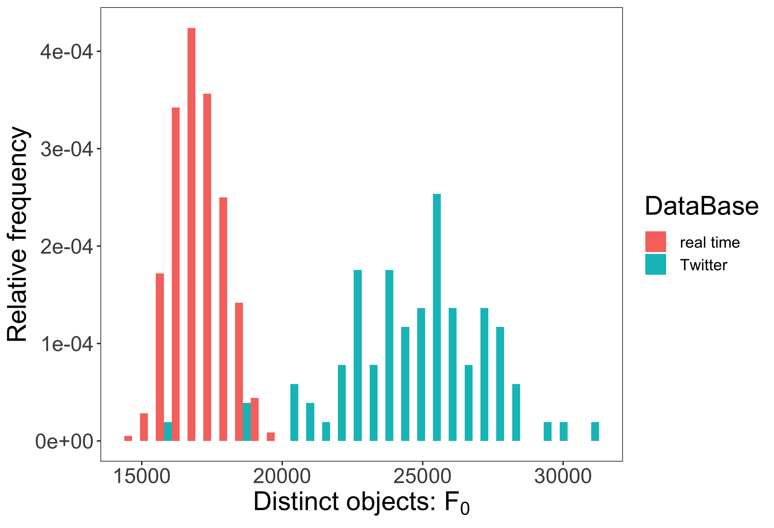
We then analyze each of the compressed files, that contains a different value of distinct object F0F_{0}. The distribution of the true F0F_{0} is plotted in Figure 5 (top-left). For each of this file, we also estimate F0F_{0} with F0^=𝕙p0−1​(λ0​𝒴)\hat{F_{0}}=\mathbbm{h}_{p_{0}}^{-1}(\lambda_{0}\mathcal{Y}), and we compute the relative accuracy of each estimation with F0^/F0\hat{F_{0}}/F_{0}. The distribution of the relative accuracy is plotted in Figure 5 (top-center) for both the databases. In Figure 5 (top-rigth), the scatterplot of the accuracy F0^/F0\hat{F_{0}}/F_{0} vs. F0F_{0} shows that there is not association between these two variables (Twitter R2=0.008839R^{2}=0.008839, p-value=0.3754\text{p-value}=0.3754, real time R2=0.0004698R^{2}=0.0004698, p-value=0.494\text{p-value}=0.494).

Refer to captionRefer to captionRefer to captionRefer to captionRefer to caption

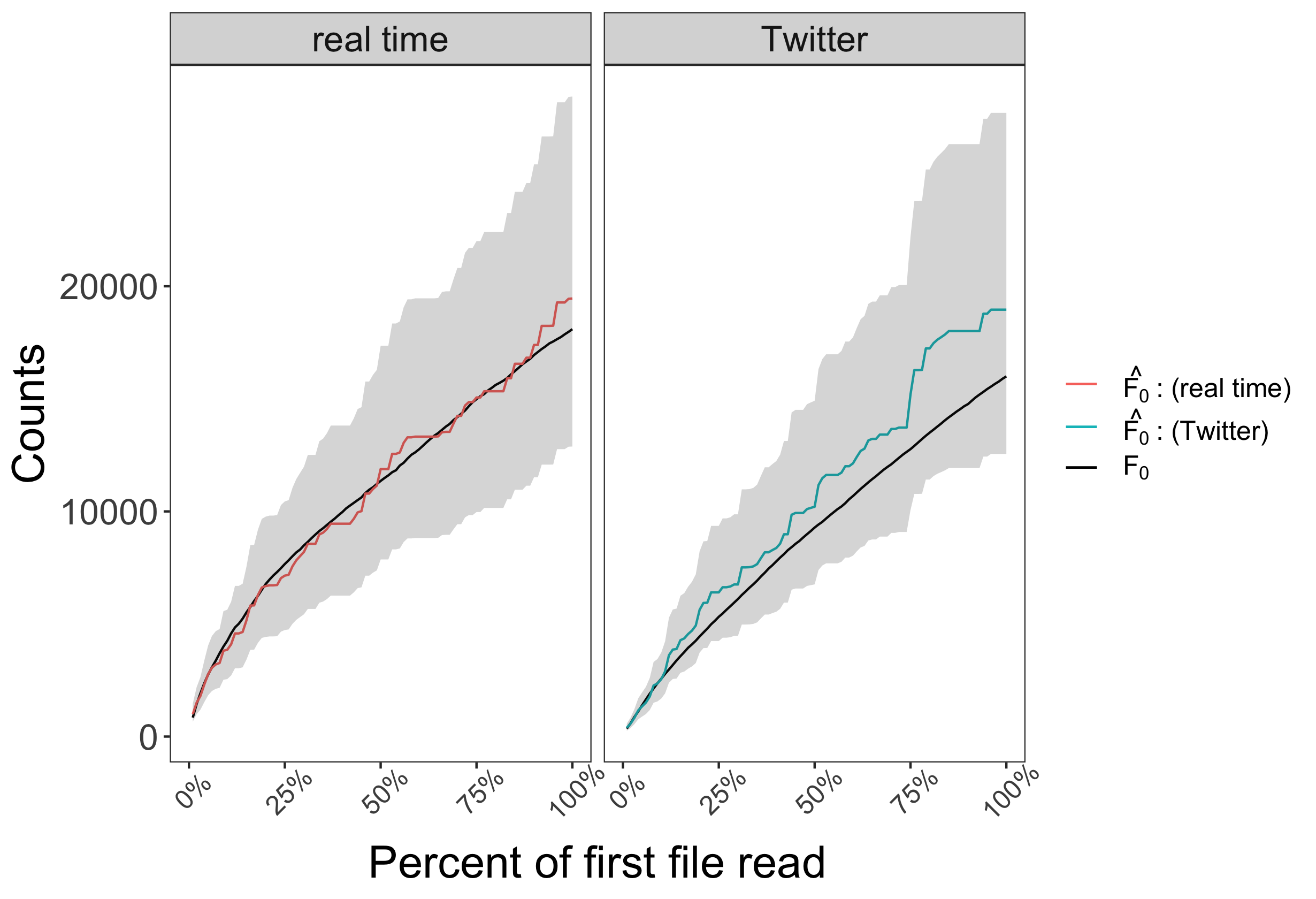
Figure 5. Analysis of accuracy of the estimations. Top-left: histogram of the number F0F_{0} of distinct object in each file. Top-center: histogram of the percent accuracy F0^/F0\hat{F_{0}}/F_{0} of the estimates of F0F_{0} made on each file. Top-right: scatterplot of the relative accuracy F0^/F0\hat{F_{0}}/F_{0} vs. the number F0F_{0} of distinct object in each file. Bottom-left: evolution of the confidence interval for F0F_{0} during the analysis of the data in the first file (in black: true value of F0F_{0}). Bottom-right: evolution of the confidence interval for F0F_{0} during the analysis of all the streaming data (in black: true value of F0F_{0}).

Finally, we analyze the data sequentially as a data stream. We check that the 90%90\% confidence interval is consistent all along the process. In Figure 5 it is shown the evolution of the confidence interval at the beginning of the stream (during the first file, bottom left) and its consistency as the number of files increases (log\log-scale, bottom left). As expected, the cold-start effect is mitigated since the approximation is not made on asymptotic properties.

7. Theoretical resolution of computational aspects

We recall that we build confidence intervals for F0F_{0} based on the output 𝕐\mathbb{Y} of Algorithm 2. For example, Algorithm 3 shows how to compute the confidence interval of the form (0,upper)(0,\mathrm{upper}) and it faces two nonlinear problems. Analogous procedures can be used to compute confidence intervals of other forms. The key computational point is the necessity of numerically solving some nonlinear equations that involve mathematical special functions.

In the following sections, we state the relevant inequalities that can be used to find the root of f⁡(x)=0f(x)=0 in our context, with the Halley’s method [24]. This iterative method is given by

xn+1=xn−2​f​(xn)​f′​(xn)2​(f′​(xn))2−f⁡(xn)​f′′​(xn),x_{n+1}=x_{n}-\frac{2f(x_{n})f^{\prime}(x_{n})}{2{\big(f^{\prime}(x_{n})\big)}^{2}-f(x_{n})f^{\prime\prime}(x_{n})},

it is essentially the Newton method applied to the function g⁡(x)=f⁡(x)|f′​(x)|g(x)=\tfrac{f(x)}{\sqrt{|f^{\prime}(x)|}}, and it achieves a cubic rate of convergence in the neighborhood of the solution, see [3].

In addition, we give accurate lower and upper bounds for the solution, that can be shown to be contained in the basin of attraction of the solution. Note that these bounds can be used also with a much simpler and robust bisection method, which has as the counterpart a linear rate of convergence.

7.1. The problem ψ⁡(x)−y=0\psi(x)-y=0

We recall here that the digamma function ψ:(0,∞)→ℝ\psi:(0,\infty)\to\mathbb{R} is defined as the logarithmic derivative of the Γ\Gamma function, see [1, §6.3], and it satisfies the relation

(8) ψ⁡(x+1)=ψ⁡(x)+1x.\psi(x+1)=\psi(x)+\tfrac{1}{x}.

In addition ψ\psi is a strictly monotone, concave function, with limt→0+ψ⁡(t)=−∞\lim_{t\to 0^{+}}\psi(t)=-\infty, ψ⁡(1)=−γ\psi(1)=-\gamma and ψ⁡(t)=log⁡(t)+o⁡(1)\psi(t)=\log(t)+o(1) when t→∞t\to\infty (see, for example, [10]). Finally, it is implemented in all the recent math packages together with its first and second derivative functions ψ1\psi_{1} and ψ2\psi_{2}.

As shown in Section S:C.1, we have

(9) ln⁡(x−12)<y<ln⁡(x),ey<x<ey+12,∀x>12,∀y=ψ⁡(x).\ln(x-\tfrac{1}{2})<y<\ln(x),\qquad e^{y}<x<e^{y}+\tfrac{1}{2},\qquad\forall x>\tfrac{1}{2},\forall y=\psi(x).

7.2. The problem 𝕙p​(x)−y=0\mathbbm{h}_{p}(x)-y=0

First note that 𝕙p​(x),𝕙p′​(x)\mathbbm{h}_{p}(x),\mathbbm{h}_{p}^{\prime}(x) and 𝕙p′′​(x)\mathbbm{h}_{p}^{\prime\prime}(x) may be computed with with arbitrary precision, because of (S:A.2) and (S:A.3) and the fact that a quad-double precision algorithm to calculate Lerch’s transcendent of real arguments have been already developed, see [2].

For p∈(0,1)p\in(0,1), as shown in [5, Section S:C.2], we have

(10) ey−γp−12≥x≥{ey−γp−e+1ln⁡(1−p)if ​y>log⁡(γ+p⁡(12−1(e−1)​ln⁡(1−p)));ey−γ−1otherwise.\frac{{e^{y-\gamma}}}{p}-\frac{1}{2}\geq x\geq\begin{cases}\frac{{e^{y-\gamma}}}{p}-e+\tfrac{1}{\ln(1-p)}&\text{if }{y}>\log\big(\gamma+p(\tfrac{1}{2}-\tfrac{1}{(e-1)\ln(1-p)})\big);\\ {e^{y-\gamma}}-1&\text{otherwise}.\end{cases}

7.3. The problem y=(x−γ)​t​(x)−ln⁡Γ⁡(1+t⁡(x))y=(x-\gamma)t(x)-\ln\Gamma(1+t(x)), where t⁡(x)=ψ−1​(x−γ)−1t(x)=\psi^{-1}(x-\gamma)-1

Note that, if g⁡(x)=(x−γ)​t​(x)−ln⁡Γ⁡(1+t⁡(x))g(x)=(x-\gamma)t(x)-\ln\Gamma(1+t(x)), then

(11) g′​(x)=t⁡(x)+t′​(x)​(x−γ−ψ⁡(1+t⁡(x)))=t⁡(x),g^{\prime}(x)=t(x)+t^{\prime}(x)(x-\gamma-\psi(1+t(x)))=t(x),

since, by definition of t⁡(x)t(x), ψ⁡(1+t⁡(x))=x−γ\psi(1+t(x))=x-\gamma. Then the formula of the derivative of the inverse function gives

g′′​(x)=t′​(x)=1ψ1​(ψ−1​(x−γ))=1ψ1​(1+t​(x)).g^{\prime\prime}(x)=t^{\prime}(x)=\frac{1}{\psi_{1}(\psi^{-1}(x-\gamma))}=\frac{1}{\psi_{1}(1+t(x))}.

As shown in [5, Section S:C.3], we have

(12) 150​y\displaystyle\sqrt{\frac{1}{50}y} <x<π​23​y,\displaystyle<x<\pi\sqrt{\frac{2}{3}y}, if y<3;\displaystyle\text{if $y<3$;}
23​(log⁡(y+12)+γ)\displaystyle\frac{2}{3}\Big(\log\Big(y+\frac{1}{2}\Big)+\gamma\Big) <x<2​(log⁡(43​y+1)+γ),\displaystyle<x<2\Big(\log\Big(\frac{4}{3}y+1\Big)+\gamma\Big), if y≥3.\displaystyle\text{if $y\geq 3$.}

7.4. The problem y=(x+γ)​t​(x)−ln⁡Γ⁡(1−t⁡(x))y=(x+\gamma)t(x)-\ln\Gamma(1-t(x)), where t⁡(x)=1−ψ−1​(−x−γ)t(x)=1-\psi^{-1}(-x-\gamma)

Note that, if g⁡(x)=(x+γ)​t​(x)−ln⁡Γ⁡(1−t⁡(x))g(x)=(x+\gamma)t(x)-\ln\Gamma(1-t(x)), then

(13) g′​(x)=t⁡(x)+t′​(x)​(x+γ−ψ⁡(1−t⁡(x)))=t⁡(x),g^{\prime}(x)=t(x)+t^{\prime}(x)(x+\gamma-\psi(1-t(x)))=t(x),

since, by definition of t⁡(x)t(x), ψ⁡(1−t⁡(x))=−x−γ\psi(1-t(x))=-x-\gamma. Then the formula of the derivative of the inverse function gives

g′′​(x)=t′​(x)=1ψ1​(ψ−1​(−x−γ))=1ψ1​(1−t​(x)).g^{\prime\prime}(x)=t^{\prime}(x)=\frac{1}{\psi_{1}(\psi^{-1}(-x-\gamma))}=\frac{1}{\psi_{1}(1-t(x))}.

As shown in [5, Section S:C.4], we have

(14) max⁡(−ln⁡(1−C)−γ,π26​C)<x<2​(y+1)2−1,\max\Big(-\ln(1-C)-\gamma,\frac{\pi^{2}}{6}C\Big)<x<2\sqrt{(y+1)^{2}-1},

where

C=1−−(y2−6+π212)+(y2−6+π212)2+4​18−π2122​18−π212∈(0,1).C=\sqrt{1-\frac{-({\tfrac{y}{2}}-{\tfrac{6+\pi^{2}}{12}})+\sqrt{({\tfrac{y}{2}}-{\tfrac{6+\pi^{2}}{12}})^{2}+4{\tfrac{18-\pi^{2}}{12}}}}{2{\tfrac{18-\pi^{2}}{12}}}}\in(0,1).

7.5. Minimum log\log-length interval

In this section, we show how to numerically compute the minimum length interval, in log\log-scale, for a given confidence α\alpha, based on the inequalities given in Theorem 4.1. The probem is set as follows: given α∈(0,1)\alpha\in(0,1), r0≥0r_{0}\geq 0, c0≥1c_{0}\geq 1, we want to solve the nonlinear minimization problem:

min⁡(hd+hu)\displaystyle\min(h_{d}+h_{u})
subject to
{α+=1−exp(−2r0c0[(hd+γ)t+−lnΓ(1−t+)]),t+=1−ψ−1(−hd−γ);α−=1−exp(−2r0c0[(hu−γ)t−−lnΓ(1+t−)]),t−=ψ−1(hu−γ)−1;α++α−≥1+α;hd,hu≥0.\displaystyle\begin{cases}{\alpha}_{+}=1-\exp\Big(-2^{{r}_{0}}c_{0}\big[(h_{d}+\gamma)t_{+}-\ln\Gamma(1-t_{+})\big]\Big),\qquad t_{+}=1-\psi^{-1}(-h_{d}-\gamma);\\ {\alpha}_{-}=1-\exp\Big(-2^{{r}_{0}}c_{0}\big[(h_{u}-\gamma)t_{-}-\ln\Gamma(1+t_{-})\big]\Big),\qquad t_{-}=\psi^{-1}(h_{u}-\gamma)-1;\\ {\alpha}_{+}+{\alpha}_{-}\geq 1+\alpha;\\ h_{d},h_{u}\geq 0.\end{cases}

The two values α+{\alpha}_{+} and α−{\alpha}_{-} are monotone functions of hdh_{d} and huh_{u}, respectively, as a consequence of (13) and (11). As a consequence, the minimum is attained when α++α−=1+α{\alpha}_{+}+{\alpha}_{-}=1+\alpha. Then, if we set x=1−α+x=1-{\alpha}_{+}, the problem above may be rewritten in terms of xx: given α∈(0,1){\alpha}\in(0,1) and a0=2r0​c0∈{1,2,…}a_{0}=2^{{r}_{0}}c_{0}\in\{1,2,\ldots\}, find

min⁡(g⁡(x))=min⁡(y+−1​(−log⁡xa0)+y−−1​(−log⁡(1−α−x)a0))\displaystyle\min(g(x))=\min\big(y_{+}^{-1}(-\tfrac{\log x}{a_{0}})+y_{-}^{-1}(-\tfrac{\log(1-{\alpha}-x)}{a_{0}})\big)
subject to
{y+(h)=(h+γ)t+−lnΓ(1−t+),t+=1−ψ−1(−h−γ);y−(h)=(h−γ)t−−lnΓ(1+t−),t−=ψ−1(h−γ)−1;0≤x≤1−α.\displaystyle\begin{cases}y_{+}(h)=(h+\gamma)t_{+}-\ln\Gamma(1-t_{+}),\qquad t_{+}=1-\psi^{-1}(-h-\gamma);\\ y_{-}(h)=(h-\gamma)t_{-}-\ln\Gamma(1+t_{-}),\qquad t_{-}=\psi^{-1}(h-\gamma)-1;\\ 0\leq x\leq 1-{\alpha}.\end{cases}

Differentiating gg with respect to xx, since y±′​(h)=t±​(h)y_{\pm}^{\prime}(h)=t_{\pm}(h) by (13) and (11), we obtain,

g′​(x)=−1a0​x​1t+​(y+−1​(−log⁡xa0))+1a0​(1−α−x)​1t−​(y−−1​(−log⁡(1−α−x)a0))g^{\prime}(x)=-\frac{1}{a_{0}x}\frac{1}{t_{+}\Big(y_{+}^{-1}\Big(-\frac{\log x}{a_{0}}\Big)\Big)}+\frac{1}{a_{0}(1-{\alpha}-x)}\frac{1}{t_{-}\Big(y_{-}^{-1}\Big(-\frac{\log(1-{\alpha}-x)}{a_{0}}\Big)\Big)}

which is null when the following equation is zero

f⁡(x)=x​t+​(y+−1​(−log⁡xa0))−(1−α−x)​t−​(y−−1​(−log⁡(1−α−x)a0))f(x)={x}{t_{+}\Big(y_{+}^{-1}\Big(-\frac{\log x}{a_{0}}\Big)\Big)}-{(1-{\alpha}-x)}{t_{-}\Big(y_{-}^{-1}\Big(-\frac{\log(1-{\alpha}-x)}{a_{0}}\Big)\Big)}

Call

t^+=t^+​(x)=t+​(y+−1​(−log⁡xa0)),t^−=t^−​(x)=t−​(y−−1​(−log⁡(1−α−x)a0)),\hat{t}_{+}=\hat{t}_{+}(x)=t_{+}\Big(y_{+}^{-1}\Big(-\frac{\log x}{a_{0}}\Big)\Big),\quad\hat{t}_{-}=\hat{t}_{-}(x)=t_{-}\Big(y_{-}^{-1}\Big(-\frac{\log(1-{\alpha}-x)}{a_{0}}\Big)\Big),

ψ1​(x)=d​ψ⁡(x)d​x\psi_{1}(x)=d\frac{\psi(x)}{dx} and ψ2​(x)=d​ψ1​(x)d​x\psi_{2}(x)=d\frac{\psi_{1}(x)}{dx}, then

d​t^+​(x)d​x=−1a0​x​1t^+​ψ1​(1−t^+),d​t^−​(x)d​x=+1a0​(1−α−x)​1t^−​ψ1​(1+t^−).d\frac{{\hat{t}_{+}}(x)}{dx}=-\frac{1}{a_{0}x}\frac{1}{\hat{t}_{+}\psi_{1}(1-\hat{t}_{+})},\qquad d\frac{{\hat{t}_{-}}(x)}{dx}=+\frac{1}{a_{0}(1-{\alpha}-x)}\frac{1}{\hat{t}_{-}\psi_{1}(1+\hat{t}_{-})}.

The problem is then to find the solution for the nonlinear problem f⁡(x)=0f(x)=0 that may be solved with the Halley’s method that involves the problems seen above, noticing that

f⁡(x)\displaystyle f(x) =x​t^+−(1−α−x)​t^−,\displaystyle={x}{\hat{t}_{+}}-{(1-{\alpha}-x)}{\hat{t}_{-}},
f′​(x)\displaystyle f^{\prime}(x) =t^+−1a0​t^+​ψ1​(1−t^+)+t^−−1a0​t^−​ψ1​(1+t^−)\displaystyle=\hat{t}_{+}-\frac{1}{a_{0}\hat{t}_{+}\psi_{1}(1-\hat{t}_{+})}+\hat{t}_{-}-\frac{1}{a_{0}\hat{t}_{-}\psi_{1}(1+\hat{t}_{-})}
f′′​(x)\displaystyle f^{\prime\prime}(x) =t+′​(1+ψ1​(1−t^+)−t^+​ψ2​(1−t^+)a0​(t^+​ψ1​(1−t^+))2)\displaystyle=t^{\prime}_{+}\Big(1+\frac{\psi_{1}(1-\hat{t}_{+})-\hat{t}_{+}\psi_{2}(1-\hat{t}_{+})}{a_{0}(\hat{t}_{+}\psi_{1}(1-\hat{t}_{+}))^{2}}\Big)
+t−′​(1+ψ1​(1+t^−)+t^+​ψ2​(1+t^−)a0​(t^−​ψ1​(1+t^−))2).\displaystyle\qquad+t^{\prime}_{-}\Big(1+\frac{\psi_{1}(1+\hat{t}_{-})+\hat{t}_{+}\psi_{2}(1+\hat{t}_{-})}{a_{0}(\hat{t}_{-}\psi_{1}(1+\hat{t}_{-}))^{2}}\Big).

and that a good starting point is given by x0=1−α2x_{0}=\tfrac{1-{\alpha}}{2}.

8. Conclusions

In this paper, we provide analytical confidence intervals for the number F0F_{0} of distinct elements in data streams by analyzing a class of FMa. While the major concern of the state of the art is algorithm’s complexity, here the new mathematical-statistical approach permits a extensive analysis of such classes of algorithms. The HyperLogLog data structure (called 𝕏\mathbb{X} in this paper) is enriched with a new data matrix of fized size (ℤ\mathbb{Z}) that helps to bound uniformly the estimators during the querying counting phase. In this phase, the Chernoff bounds may be applied analytically and gives asymptotically efficient estimators that are related to the extreme value theory. In addition, the relation E⁡(𝒴¯)=𝕙p0​(F0)λ0E(\bar{\mathcal{Y}})=\frac{\mathbbm{h}_{p_{0}}(F_{0})}{\lambda_{0}} introduces a new class of special functions 𝕙p0\mathbbm{h}_{p_{0}} used to find the confidence interval.

Since the new theoretical results are based on some analytical, computational and numerical assumptions, we have shown that these assumptions are always satisfied in real situations. First, the analytical asymptotic approximation made on Chernoff bounds is shown to be irrelevant when F0F_{0} is large. Then, statistical assumptions on the distributions of the quantities of interests are shown to be satisfied on a real dataset and the accuracy of the methodology is provided. Finally, the computational solution of the problems related to the new special functions is solved by showing the basins of attraction for a Newton based method with cubic rate of convergence.

References

  • [1] M. Abramowitz and I. A. Stegun. Handbook of mathematical functions with formulas, graphs, and mathematical tables, volume 55 of National Bureau of Standards Applied Mathematics Series. For sale by the Superintendent of Documents, U.S. Government Printing Office, Washington, D.C., 1964.
  • [2] S. V. Aksenov, M. A. Savageau, U. D. Jentschura, J. Becher, G. Soff, and P. J. Mohr. Application of the combined nonlinear-condensation transformation to problems in statistical analysis and theoretical physics. Computer Physics Communications, 150(1):1 – 20, 2003.
  • [3] G. Alefeld. On the convergence of halley’s method. The American Mathematical Monthly, 88(7):530–536, 1981.
  • [4] G. Aletti. Generation of discrete random variables in scalable frameworks. Statist. Probab. Lett., 132:99–106, 2018.
  • [5] G. Aletti. Supplementary material for “Analytical confidence intervals for the number of different objects in data streams”. arXiv:1909.11564, 2020.
  • [6] N. Alon, Y. Matias, and M. Szegedy. The space complexity of approximating the frequency moments. In Proceedings of the Twenty-eighth Annual ACM Symposium on Theory of Computing, STOC ’96, pages 20–29, New York, NY, USA, 1996. ACM.
  • [7] B. C. Arnold, N. Balakrishnan, and H. N. Nagaraja. A first course in order statistics, volume 54 of Classics in Applied Mathematics. Society for Industrial and Applied Mathematics (SIAM), Philadelphia, PA, 2008. Unabridged republication of the 1992 original.
  • [8] B. Babcock, S. Babu, M. Datar, R. Motwani, and J. Widom. Models and issues in data stream systems. In Proceedings of the Twenty-first ACM SIGMOD-SIGACT-SIGART Symposium on Principles of Database Systems, PODS ’02, pages 1–16, New York, NY, USA, 2002. ACM.
  • [9] Z. Bar-Yossef, T. S. Jayram, R. Kumar, D. Sivakumar, and L. Trevisan. Counting distinct elements in a data stream. In J. D. P. Rolim and S. Vadhan, editors, Randomization and Approximation Techniques in Computer Science, pages 1–10, Berlin, Heidelberg, 2002. Springer Berlin Heidelberg.
  • [10] H. G. Diamond and A. Straub. Bounds for the logarithm of the euler gamma function and its derivatives. Journal of Mathematical Analysis and Applications, 433(2):1072 – 1083, 2016.
  • [11] M. Durand and P. Flajolet. Loglog counting of large cardinalities (extended abstract). Lecture Notes in Computer Science (including subseries Lecture Notes in Artificial Intelligence and Lecture Notes in Bioinformatics), 2832:605–617, 2003.
  • [12] O. Ertl. New cardinality estimation algorithms for hyperloglog sketches, 2017. preprint at http://oertl.github.io/hyperloglog-sketch-estimation-paper/.
  • [13] C. Estan, G. Varghese and M. Fisk. Bitmap algorithms for counting active flows on high-speed links. IEEE/ACM Transactions on Networking, 14(5):925–937, 2006.
  • [14] P. Flajolet. Approximate counting: A detailed analysis. BIT Numerical Mathematics, 25(1):113–134, Mar 1985.
  • [15] P. Flajolet, É. Fusy, O. Gandouet, and F. Meunier. HyperLogLog: the analysis of a near-optimal cardinality estimation algorithm. In 2007 Conference on Analysis of Algorithms, AofA 07, Discrete Math. Theor. Comput. Sci. Proc., AH, pages 127–145. Assoc. Discrete Math. Theor. Comput. Sci., Nancy, 2007.
  • [16] P. Flajolet and G. N. Martin. Probabilistic counting algorithms for data base applications. Journal of Computer and System Sciences, 31(2):182–209, 1985.
  • [17] O. Gandouet and A. Jean-Marie. LogLog counting for the estimation of IP traffic. In Fourth Colloquium on Mathematics and Computer Science Algorithms, Trees, Combinatorics and Probabilities, Discrete Math. Theor. Comput. Sci. Proc., AG, pages 119–128. Assoc. Discrete Math. Theor. Comput. Sci., Nancy, 2006.
  • [18] B. Gnedenko. Sur la distribution limite du terme maximum d’une serie aleatoire. Annals of Mathematics, 44(3):423–453, 1943.
  • [19] D. M. Kane, J. Nelson, and D. P. Woodruff. An optimal algorithm for the distinct elements problem. In Proceedings of the Twenty-ninth ACM SIGMOD-SIGACT-SIGART Symposium on Principles of Database Systems, PODS ’10, pages 41–52, New York, NY, USA, 2010. ACM.
  • [20] National Institute of Standards and Technology (NIST). CRYPTOGRAPHIC TOOLKIT. online at http://csrc.nist.gov/groups/ST/toolkit/rng/.
  • [21] National Institute of Standards and Technology (NIST). Guide to NIST’s tests. online at http://csrc.nist.gov/groups/ST/toolkit/rng/stats_tests.html.
  • [22] National Institute of Standards and Technology (NIST). References. online at http://csrc.nist.gov/groups/ST/toolkit/rng/references.html.
  • [23] P. Jia, P. Wang, J. Zhao, J. Tao, Y. Yuan and X. Guan. Erasable virtual hyperloglog for approximating cumulative distribution over data streams. IEEE Transactions on Knowledge and Data Engineering, 2021.
  • [24] T. R. Scavo and J. B. Thoo. On the geometry of halley’s method. The American Mathematical Monthly, 102(5):417–426, 1995.
  • [25] K.-Y. Whang, B. T. Vander-Zanden and H. M. Taylor. A linear-time probabilistic counting algorithm for database applications. ACM Trans. Database Syst., 15(2):208–-229, 1990.
  • [26] Q. Xiao, S. Chen, Y. Zhou, M. Chen, J. Luo, T. Li and Y. Ling. Cardinality estimation for elephant flows: a compact solution based on virtual register sharing. IEEE/ACM Transactions on Networking, 25(6):3738–3752, 2017.

Supplementary Material

In this document we collect some technical results useful for [3]. Therefore, the notation and the assumptions used here are the same as those used in that paper. The reference to that paper are proceeded with a M, so that (M:11) will refer to the equation (1)(1) in [3].

Supplementary Material A Special functions used in the paper

Modification of the harmonic numbers and Lerch transcendent function

For any integer number mm, we denote by 𝕙⁡(m)\mathbbm{h}(m) the m{m}-th harmonic number. We recall here that

(A.1) 𝕙⁡(m)=ψ⁡(m+1)+γ=∑j=1m1j=∑j=0m−1∫01tj​𝑑t=∫011−tm1−t​𝑑t,\mathbbm{h}(m)=\psi(m+1)+\gamma=\sum_{j=1}^{m}\frac{1}{j}=\sum_{j=0}^{m-1}\int_{0}^{1}t^{j}\,dt=\int_{0}^{1}\frac{1-t^{m}}{1-t}\,dt,

where ψ\psi is the derivative of the logarithm of gamma function (also called digamma function). The constant γ\gamma is the Euler–Mascheroni constant throughout the whole paper. The function 𝕙\mathbbm{h} can be extended therefore to the real non-negative numbers, by setting 𝕙1​(x)=∫011−tx1−t​𝑑t\mathbbm{h}_{1}(x)=\int_{0}^{1}\frac{1-t^{x}}{1-t}\,dt, which is known as the integral representation given by Euler.

Definition A.1.

For 0≤p≤10\leq p\leq 1, x≥0x\geq 0, we define the pp-modification of the harmonic numbers 𝕙p​(x)\mathbbm{h}_{p}(x), where

𝕙p​(x)=∫011−(1−p+p​t)x1−t​𝑑t,\mathbbm{h}_{p}(x)=\int_{0}^{1}\frac{1-(1-p+pt)^{x}}{1-t}\,dt,

The function 𝕙p​(x)\mathbbm{h}_{p}(x) has the following properties

  • •

    𝕙p​(0)=0\mathbbm{h}_{p}(0)=0, 𝕙0​(x)=0\mathbbm{h}_{0}(x)=0, 𝕙p​(1)=p\mathbbm{h}_{p}(1)=p and 𝕙1​(x)=𝕙​(x)\mathbbm{h}_{1}(x)=\mathbbm{h}(x) by definition;

  • •

    with two changes of integration variable z=(1−p⁡(1−t))z=(1-p(1-t)) and z=(1−p)​e−wz=(1-p)e^{-w}, we we may rewrite 𝕙p​(x)\mathbbm{h}_{p}(x) as

    (A.2) 𝕙p​(x)\displaystyle\mathbbm{h}_{p}(x) =∫1−p11−zx1−z​𝑑z=ψ⁡(x+1)+γ−∫01−p1−zx1−z​𝑑z\displaystyle=\int_{1-p}^{1}\frac{1-z^{x}}{1-z}\,dz=\psi(x+1)+\gamma-\int_{0}^{1-p}\frac{1-z^{x}}{1-z}\,dz
    =ψ⁡(x+1)+γ+log⁡p+∫01−pzx1−z​𝑑z\displaystyle=\psi(x+1)+\gamma+\log p+\int_{0}^{1-p}\frac{z^{x}}{1-z}\,dz
    =ψ⁡(x+1)+γ+log⁡p+(1−p)x+1​∫0∞e−w⁡(x+1)1−(1−p)​e−w​𝑑w\displaystyle=\psi(x+1)+\gamma+\log p+(1-p)^{x+1}\int_{0}^{\infty}\frac{e^{-w(x+1)}}{1-(1-p)e^{-w}}\,dw
    =ψ⁡(x+1)+γ+log⁡p+(1−p)x+1​Φ​(1−p,1,x+1),\displaystyle=\psi(x+1)+\gamma+\log p+(1-p)^{x+1}\,\Phi(1-p,1,x+1),

    where Φ\Phi is the Lerch transcendent function, see [6], and the last equality is a consequence of the following equation, valid for m∈ℕm\in\mathbb{N} and z=(1−p)z=(1-p):

    Φ⁡(z,s,a)=zm​Φ​(z,s,a+m)+∑n=0m−1zn(a+n)s.\Phi\left(z,s,a\right)=z^{m}\Phi\left(z,s,a+m\right)+\sum_{n=0}^{m-1}\frac{z^{n}}{(a+n)^{s}}.
  • •

    By (A.2), 𝕙p​(x)\mathbbm{h}_{p}(x) is strictly increasing and continuous, both as a function of xx and pp. In addition, for any p>0p>0, limx→∞𝕙p​(x)=+∞\lim_{x\to\infty}\mathbbm{h}_{p}(x)=+\infty, and hence 𝕙p:[0,+∞)→[0,+∞)\mathbbm{h}_{p}:[0,+\infty)\to[0,+\infty) is an isomorphism (continuous invertible function, with continuous inverse function). Its inverse function (𝕙p)−1:[0,+∞)→[0,+∞)(\mathbbm{h}_{p})^{-1}:[0,+\infty)\to[0,+\infty) is hence well-defined and it is used in the paper.

The Lerch transcendent function appears also in the derivatives of 𝕙p\mathbbm{h}_{p}. Denote by

Φ1=Φ⁡(1−p,1,x+1),Φ2=Φ⁡(1−p,2,x+1),Φ3=Φ⁡(1−p,3,x+1),\Phi_{1}=\Phi(1-p,1,x+1),\qquad\Phi_{2}=\Phi(1-p,2,x+1),\qquad\Phi_{3}=\Phi(1-p,3,x+1),

and note that Φn+1=−n∂Φn∂x\Phi_{n+1}=-n\partial\frac{\Phi_{n}}{\partial x}; by (A.2) we get

(A.3) 𝕙p′​(x)\displaystyle\mathbbm{h}_{p}^{\prime}(x) =∂ψ⁡(x+1)+γ+log⁡p+(1−p)x+1⋅Φ⁡(1−p,1,x+1)∂x\displaystyle=\partial\frac{\psi(x+1)+\gamma+\log p+(1-p)^{x+1}\cdot\Phi(1-p,1,x+1)}{\partial x}
=ψ1​(x+1)+(1−p)x+1​(log⁡(1−p)⋅Φ1−Φ2)\displaystyle=\psi_{1}(x+1)+(1-p)^{x+1}(\log(1-p)\cdot\Phi_{1}-\Phi_{2})
𝕙p′′​(x)\displaystyle\mathbbm{h}_{p}^{\prime\prime}(x) =ψ2​(x+1)+(1−p)x+1​((log⁡(1−p))2⋅Φ1−2​log⁡(1−p)⋅Φ2+2​Φ3).\displaystyle=\psi_{2}(x+1)+(1-p)^{x+1}((\log(1-p))^{2}\cdot\Phi_{1}-2\log(1-p)\cdot\Phi_{2}+2\Phi_{3}).

Product representation and incomplete Gamma function

For what concerns the infinite product representation of the Gamma function

Γ(z)=limK→∞e−γ​zz∏k=1K(1+zk)−1ezk,z≠−1,−2,…,\Gamma(z)=\lim_{K\to\infty}\frac{e^{-\gamma z}}{z}\prod_{k=1}^{K}\left(1+\frac{z}{k}\right)^{-1}e^{\frac{z}{k}},\qquad z\neq-1,-2,\ldots,

given by Schlömilch in 1844 and Newman in 1848, if we evaluate it in z=±tz=\pm t, we obtain

(A.4) Γ⁡(1−t)​e−γ​t=∏j=1∞e−tj1−tj,t∈(0,1),Γ⁡(1+t)​eγ​t=∏j=1∞etj1+tj,t>0.\Gamma(1-t)e^{-\gamma t}=\prod_{j=1}^{\infty}\frac{e^{-\frac{t}{j}}}{1-\frac{t}{j}},\ t\in(0,1),\qquad\Gamma(1+t)e^{\gamma t}=\prod_{j=1}^{\infty}\frac{e^{\frac{t}{j}}}{1+\frac{t}{j}},\ t>0.

Finally, for x>0x>0, we denote by E1​(x)E_{1}(x) the exponential integral (or incomplete gamma function). As shown in [1, p. 229, 5.1.20], we have that

(A.5) E1​(x)=∫x∞e−tt​𝑑t<e−x​ln⁡(1+1x).E_{1}(x)=\int_{x}^{\infty}\frac{e^{-t}}{t}\,dt<e^{-x}\,\ln\!\Big(1+\frac{1}{x}\Big).

Note that, if p∈(0,1)p\in(0,1) and t=−ln⁡(1−p)​wt=-\ln(1-p)w,

E1​(x)=∫x∞e−tt​𝑑t=∫−xln⁡(1−p)∞(1−p)ww​𝑑w.E_{1}(x)=\int_{x}^{\infty}\frac{e^{-t}}{t}\,dt=\int_{-\tfrac{x}{\ln(1-p)}}^{\infty}\frac{(1-p)^{w}}{w}\,dw.

We will make use of the very well known formula −ln⁡(p)=∑j=1∞(1−p)jj-\ln(p)=\sum_{j=1}^{\infty}\frac{(1-p)^{j}}{j}. To bound the tail of the series, we immediately obtain by (A.5) that, for any x>0x>0,

(A.6) ∑j=0∞(1−p)x+j+1x+j+1≤∫x∞(1−p)ww​dw=E1​(−x​ln⁡(1−p))<ex​ln⁡(1−p)​ln⁡(1−1x​ln⁡(1−p)).\sum_{j=0}^{\infty}\frac{(1-p)^{x+j+1}}{x+j+1}\leq\int_{x}^{\infty}\frac{(1-p)^{w}}{w}\,dw=E_{1}(-x\ln({1-p}))\\ <e^{x\ln({1-p})}\,\ln\!\Big(1-\frac{1}{x\ln({1-p})}\Big).

The next representation lemma is used both in the analytical and in the numerical part of the paper.

Lemma A.2.

Let x>0x>0 be fixed. Then the functions

g+​(t)\displaystyle g_{+}(t) =(x+γ)​t−ln⁡Γ⁡(1−t),t∈(0,1)\displaystyle=(x+\gamma)t-\ln\Gamma(1-t),\qquad t\in(0,1)
g−​(t)\displaystyle g_{-}(t) =(x−γ)​t−ln⁡Γ⁡(1+t),t>0\displaystyle=(x-\gamma)t-\ln\Gamma(1+t),\qquad t>0

attain their (strictly positive) maxima at the points t+=1−ψ−1​(−x−γ)t_{+}=1-\psi^{-1}(-x-\gamma) and t−=ψ−1​(x−γ)−1t_{-}=\psi^{-1}(x-\gamma)-1, respectively.

Proof.

We give the proof for g+g_{+}, since the same arguments apply to g−g_{-}. We have

  • •

    g+​(t)g_{+}(t) is concave, since ln⁡Γ⁡(1−t)\ln\Gamma(1-t) is a convex analytic function on (0,1)(0,1);

  • •

    g+​(0)=ln⁡Γ⁡(1)=0g_{+}(0)=\ln\Gamma(1)=0, g+′​(0)=(x+γ)+ψ⁡(1)=x>0g_{+}^{\prime}(0)=(x+\gamma)+\psi(1)=x>0;

  • •

    limt→1g+​(t)=−∞\lim_{t\to 1}g_{+}(t)=-\infty;

and hence the maximum of g+g_{+} on (0,1)(0,1) is strictly positive. The maximum point t+t_{+} is attained when g+′​(t+)=0g_{+}^{\prime}(t_{+})=0, that is when (x+γ)+ψ⁡(1+t+)=0(x+\gamma)+\psi(1+t_{+})=0. ∎

Supplementary Material B Proof of some technical results of [3]

B.1. Proof of 0<Yr​c−Y¯r​c<2−z0λ00<{Y}_{r\,c}-\bar{Y}_{r\,c}<\tfrac{2^{-z_{0}}}{\lambda_{0}} in [3, Lemma 3.1]

We recall here that

2−z0​Z​(c,o)=∑z=1z0sz∗​2−z,Z¯​(o,c)=∑z=1∞sz∗​2−z2^{-z_{0}}Z(c,o)=\sum_{z=1}^{z_{0}}s^{*}_{z}2^{-z},\qquad\bar{Z}(o,c)=\sum_{z=1}^{\infty}s^{*}_{z}2^{-z}

and with

Y⁡(o,c)=X⁡(c,o)−log2⁡(1+2−z0​Z​(c,o)),Y¯​(o,c)=(X⁡(c,o)−log2⁡(1+Z¯​(o,c))CLOSE,{Y}(o,c)=X(c,o)-\log_{2}(1+2^{-z_{0}}Z(c,o)),\qquad\bar{Y}(o,c)=\big(X(c,o)-\log_{2}(1+\bar{Z}(o,c)),

by definition of Yr​c{Y}_{r\,c} and Y¯r​c\bar{Y}_{r\,c}, we get

Yr​c−Y¯r​c\displaystyle{Y}_{r\,c}-\bar{Y}_{r\,c} =max{o:R⁡(o,c)=r}(Y(o,c)−Y¯(o,c))\displaystyle=\max_{\{o\colon R(o,c)=r\}}({Y}(o,c)-\bar{Y}(o,c))
=max{o:R⁡(o,c)=r}(−log2(1+2−z0Z(c,o))+log2(1+Z¯(c,o)))\displaystyle=\max_{\{o\colon R(o,c)=r\}}\big(-\log_{2}(1+2^{-z_{0}}Z(c,o))+\log_{2}(1+\bar{Z}(c,o))\big)
=max{o:R⁡(o,c)=r}log2(1+2−z0​∑z=z0+1∞sz∗​2−z1+∑z=1z0sz∗​2−z).\displaystyle=\max_{\{o\colon R(o,c)=r\}}\log_{2}\Big(1+\frac{2^{-z_{0}}\sum_{z=z_{0}+1}^{\infty}s^{*}_{z}2^{-z}}{1+\sum_{z=1}^{z_{0}}s^{*}_{z}2^{-z}}\Big).

Now, note that

0<∑z=1∞sz∗​2−z1+∑z=1z0sz∗​2−z<10<\frac{\sum_{z=1}^{\infty}s^{*}_{z}2^{-z}}{1+\sum_{z=1}^{z_{0}}s^{*}_{z}2^{-z}}<1

and then, since ln⁡(1+x)<x\ln(1+x)<x for x>0x>0,

0<log2⁡(1+2−z0​∑z=z0+1∞sz∗​2−z1+∑z=1z0sz∗​2−z)<2−z0ln⁡(2)=2−z0λ0.0<\log_{2}\Big(1+\frac{2^{-z_{0}}\sum_{z=z_{0}+1}^{\infty}s^{*}_{z}2^{-z}}{1+\sum_{z=1}^{z_{0}}s^{*}_{z}2^{-z}}\Big)<\frac{2^{-z_{0}}}{\ln(2)}=\frac{2^{-z_{0}}}{\lambda_{0}}.

B.2. Detailed proof of [3, Theorem 4.1]

First step. By [3, Lemma 3.1], it is possible to calculate the moment-generating function of 𝒴¯\bar{\mathcal{Y}}, conditioned on {𝒎c,c=1,…,c0}\{\boldsymbol{m}_{c},c=1,\ldots,c_{0}\}. In fact, since

(B.1) Y¯r​c=maxo1,…,omr​c:R⁡(c,oj)=roj​ different objects(Y¯(oj,c)),\bar{Y}_{r\,c}=\max_{\begin{subarray}{c}o_{1},\ldots,o_{m_{r\,c}}\colon R(c,o_{j})=r\\ o_{j}\text{ different objects}\end{subarray}}\big(\bar{Y}(o_{j},c)\big),

it is well known [7] that the moment generating function of the max of exponential random variables is

E⁡(es​Y¯r​c|{𝒎c,c=1,…,c0})=∏j=1mr​c(1−sλ0​j)−1,0<s<λ0E(e^{s\bar{Y}_{r\,c}}|\{\boldsymbol{m}_{c},c=1,\ldots,c_{0}\})=\prod_{j=1}^{m_{r\,c}}(1-\tfrac{s}{\lambda_{0}j})^{-1},\qquad 0<s<\lambda_{0}

which implies, for 0<s<c0​2r0​λ00<s<{c_{0}}2^{r_{0}}\lambda_{0},

E⁡(es​𝒴¯|{𝒎c,c=1,…,c0})=E⁡(es​∑c=1c0∑r=12r0Y¯r​cc0​2r0|{𝒎c,c=1,…,c0})=∏c=1c0∏r=12r0∏j=1mr​c(1−sj​c0​2r0​λ0)−1.E(e^{s\bar{\mathcal{Y}}}|\{\boldsymbol{m}_{c},c=1,\ldots,c_{0}\})=E\Big(e^{s\sum_{c=1}^{{c_{0}}}\sum_{r=1}^{2^{r_{0}}}\tfrac{\bar{Y}_{r\,c}}{{c_{0}2^{r_{0}}}}}\Big|\{\boldsymbol{m}_{c},c=1,\ldots,c_{0}\}\Big)\\ =\prod_{c=1}^{{c_{0}}}\prod_{r=1}^{2^{r_{0}}}\prod_{j=1}^{m_{r\,c}}(1-\tfrac{s}{j{c_{0}}2^{r_{0}}\lambda_{0}})^{-1}.

Again, by (B.1)

(B.2) E⁡(Yr​c|{𝒎c,c=1,…,c0})=∑j=1mr​c1j​λ0E(Y_{r\,c}|\{\boldsymbol{m}_{c},c=1,\ldots,c_{0}\})=\sum_{j=1}^{m_{r\,c}}\frac{1}{j\lambda_{0}}

which means that

E⁡(𝒴¯|{𝒎c,c=1,…,c0})=1c0​2r0​λ0​∑c=1c0∑r=12r0∑j=1mr​c1j.E({\bar{\mathcal{Y}}}|\{\boldsymbol{m}_{c},c=1,\ldots,c_{0}\})=\frac{1}{c_{0}2^{r_{0}}\lambda_{0}}\sum_{c=1}^{{c_{0}}}\sum_{r=1}^{2^{r_{0}}}\sum_{j=1}^{m_{r\,c}}\frac{1}{j}.

Then, conditioned on {𝒎c,c=1,…,c0}\{\boldsymbol{m}_{c},c=1,\ldots,c_{0}\}, the Chernoff bound for the first inequality that concerns α+\alpha_{+} may be computed as

P⁡(𝒴¯≥E⁡(𝒴¯|{𝒎c,c=1,…,c0})+hdλ0|{𝒎c,c=1,…,c0})≤mins>0⁡e−s⁡(E⁡(𝒴¯|{𝒎c,c=1,…,c0})+hdλ0)​E​(es​𝒴¯|{𝒎c,c=1,…,c0})=mins>0⁡e−hdλ0​s​∏c=1c0∏r=12r0∏j=1mr​ce−sj​c0​2r0​λ01−sj​c0​2r0​λ0.P\Big(\bar{\mathcal{Y}}\geq E(\bar{\mathcal{Y}}|\{\boldsymbol{m}_{c},c=1,\ldots,c_{0}\})+\frac{h_{d}}{\lambda_{0}}\Big|\{\boldsymbol{m}_{c},c=1,\ldots,c_{0}\}\Big)\\ \begin{aligned} &\leq\min_{s>0}e^{-s\big({E(\bar{\mathcal{Y}}|\{\boldsymbol{m}_{c},c=1,\ldots,c_{0}\})+\frac{h_{d}}{\lambda_{0}}}\big)}E(e^{s\bar{\mathcal{Y}}}|\{\boldsymbol{m}_{c},c=1,\ldots,c_{0}\})\\ &=\min_{s>0}e^{-\tfrac{{h_{d}}}{\lambda_{0}}s}\prod_{c=1}^{{c_{0}}}\prod_{r=1}^{2^{r_{0}}}\prod_{j=1}^{m_{r\,c}}\frac{e^{-\tfrac{s}{jc_{0}2^{r_{0}}\lambda_{0}}}}{1-\tfrac{s}{j{c_{0}}2^{r_{0}}\lambda_{0}}}.\end{aligned}

Define t=sc0​2r0​λ0t=\frac{s}{{c_{0}}2^{r_{0}}\lambda_{0}}. Since exp−t1−t≥1\frac{\exp^{-t}}{1-t}\geq 1 for any t<1t<1, then for t∈(0,1)t\in(0,1), the abobe relation continues as

mins>0⁡e−hdλ0​s​∏c=1c0∏r=12r0∏j=1mr​ce−sj​c0​2r0​λ01−sj​c0​2r0​λ0\displaystyle\min_{s>0}e^{-\tfrac{{h_{d}}}{\lambda_{0}}s}\prod_{c=1}^{{c_{0}}}\prod_{r=1}^{2^{r_{0}}}\prod_{j=1}^{m_{r\,c}}\frac{e^{-\tfrac{s}{jc_{0}2^{r_{0}}\lambda_{0}}}}{1-\tfrac{s}{j{c_{0}}2^{r_{0}}\lambda_{0}}} =mint>0⁡e−t​hd​c0​2r0​∏c=1c0∏r=12r0∏j=1mr​ce−tj1−tj\displaystyle=\min_{t>0}e^{-t{h_{d}}{c_{0}}2^{r_{0}}}\prod_{c=1}^{{c_{0}}}\prod_{r=1}^{2^{r_{0}}}\prod_{j=1}^{m_{r\,c}}\frac{e^{-\tfrac{t}{j}}}{1-\tfrac{t}{j}}
≤mint>0⁡e−t​hd​c0​2r0​∏c=1c0∏r=12r0∏j=1∞e−tj1−tj\displaystyle\leq\min_{t>0}e^{-t{h_{d}}{c_{0}}2^{r_{0}}}\prod_{c=1}^{{c_{0}}}\prod_{r=1}^{2^{r_{0}}}\prod_{j=1}^{\infty}\frac{e^{-\tfrac{t}{j}}}{1-\tfrac{t}{j}}
=mint>0⁡e−t​hd​c0​2r0​∏c=1c0∏r=12r0(Γ⁡(1−t)​e−γ​t)\displaystyle=\min_{t>0}e^{-t{h_{d}}{c_{0}}2^{r_{0}}}\prod_{c=1}^{{c_{0}}}\prod_{r=1}^{2^{r_{0}}}\Big(\Gamma(1-t)e^{-\gamma t}\Big)
=exp⁡(−c0​2r0​maxt∈(0,1)​[(hd+γ)​t−ln⁡Γ⁡(1−t)]).\displaystyle=\exp\Big(-{c_{0}}2^{r_{0}}\max_{t\in(0,1)}\big[(h_{d}+\gamma)t-\ln\Gamma(1-t)\big]\Big).

The relevant aspect of the last expression is that it does not depend on {𝒎c,c=1,…,c0}\{\boldsymbol{m}_{c},c=1,\ldots,c_{0}\}, and what remains to prove is that the maximum of (hd+γ)​t−ln⁡Γ⁡(1−t)(h_{d}+\gamma)t-\ln\Gamma(1-t) on (0,1)(0,1) is attained at t+=1−ψ−1​(−hd−γ)t_{+}=1-\psi^{-1}(-h_{d}-\gamma). This is obvious, since −ln⁡Γ⁡(1−t)-\ln\Gamma(1-t) is a concave function with derivative in zero equal to −γ-\gamma, its limit is −∞-\infty as it approches 1−1^{-} and the digamma function ψ\psi is the derivative of the logarithm of the gamma function.

The proof of the second inequality that concerns α−\alpha_{-} may be done with the same ideas. In fact, the Chernoff bound may be uniformly bounded by

P⁡(𝒴¯≤E⁡(𝒴¯|{𝒎c,c=1,…,c0})−huλ0|{𝒎c,c=1,…,c0})≤mint>0⁡exp⁡(−c0​2r0​maxt>0​[(hu−γ)​t−ln⁡Γ⁡(1+t)]).P\Big(\bar{\mathcal{Y}}\leq E(\bar{\mathcal{Y}}|\{\boldsymbol{m}_{c},c=1,\ldots,c_{0}\})-\frac{h_{u}}{\lambda_{0}}\Big|\{\boldsymbol{m}_{c},c=1,\ldots,c_{0}\}\Big)\\ \leq\min_{t>0}\exp\Big(-{c_{0}}2^{r_{0}}\max_{t>0}\big[(h_{u}-\gamma)t-\ln\Gamma(1+t)\big]\Big).

Now, it is sufficient to note that −ln⁡Γ⁡(1+t)-\ln\Gamma(1+t) is a concave function with derivative in zero equal to γ\gamma, its limit is −∞-\infty as it approches +∞+\infty and the digamma function ψ\psi is again the derivative of the logarithm of the gamma function.

Second step. Starting from (B.2), note that the mr​cm_{r\,c}-armonic number may be represented in the following way:

∑j=1mr​c1j=∫011−vmr​c1−v​𝑑v=𝕙1​(mr​c).\sum_{j=1}^{m_{r\,c}}\frac{1}{j}=\int_{0}^{1}\frac{1-v^{m_{r\,c}}}{1-v}\,dv=\mathbbm{h}_{1}(m_{r\,c}).

Recall that, by [3, Lemma 3.1], mr​cm_{r\,c} is distributed as a binomial distribution, with F0F_{0} trials and probability p0=2−r0p_{0}={2^{-{r}_{0}}}. Then

λ0​E​(Yr​c)\displaystyle\lambda_{0}E(Y_{r\,c}) =λ0​E​(E⁡(Yr​c|{𝒎c,c=1,…,c0}))=E⁡(𝕙1​(mr​c))\displaystyle=\lambda_{0}E(E(Y_{r\,c}|\{\boldsymbol{m}_{c},c=1,\ldots,c_{0}\}))=E(\mathbbm{h}_{1}(m_{r\,c}))
=∑m=0F0𝕙1​(m)​(F0m)​p0m​(1−p0)F0−m\displaystyle=\sum_{m=0}^{F_{0}}\mathbbm{h}_{1}(m)\binom{{F_{0}}}{m}{p_{0}}^{m}(1-{p_{0}})^{{F_{0}}-m}
=∑m=0F0(∫011−vm1−v​𝑑v)​(F0m)​p0m​(1−p0)F0−m\displaystyle=\sum_{m=0}^{F_{0}}\Big(\int_{0}^{1}\frac{1-v^{m}}{1-v}\,dv\Big)\binom{{F_{0}}}{m}{p_{0}}^{m}(1-{p_{0}})^{{F_{0}}-m}
=∫0111−v​(∑m=0F0(1−vm)​(F0m)​p0m​(1−p0)F0−m)​𝑑v\displaystyle=\int_{0}^{1}\frac{1}{1-v}\Big(\sum_{m=0}^{F_{0}}(1-v^{m})\binom{{F_{0}}}{m}{p_{0}}^{m}(1-{p_{0}})^{{F_{0}}-m}\Big)dv
=∫0111−v​(∑m=0F0(F0m)​p0m​(1−p0)F0−mCLOSE\displaystyle=\int_{0}^{1}\frac{1}{1-v}\Big(\sum_{m=0}^{F_{0}}\binom{{F_{0}}}{m}{p_{0}}^{m}(1-{p_{0}})^{{F_{0}}-m}
−∑m=0F0(F0m)(p0v)m(1−p0)F0−m)dv\displaystyle\qquad\qquad-\sum_{m=0}^{F_{0}}\binom{{F_{0}}}{m}({p_{0}}v)^{m}(1-{p_{0}})^{{F_{0}}-m}\Big)dv
=∫011−(1−p0+p0​v)F01−v​𝑑v=𝕙p0​(F0).\displaystyle=\int_{0}^{1}\frac{1-(1-{p_{0}}+{p_{0}}v)^{F_{0}}}{1-v}\,dv=\mathbbm{h}_{p_{0}}(F_{0}).

Then, by linearity, we conclude that E⁡(𝒴¯)=𝕙p0​(F0)λ0E(\bar{\mathcal{Y}})=\frac{\mathbbm{h}_{p_{0}}(F_{0})}{\lambda_{0}}.

Supplementary Material C Lower and upper bounds of some numerical problems

C.1. Bounds of y=ψ⁡(x)y=\psi(x)

As shown in [4, Example 2.1], we may bound ψ\psi from below in the following way. The Jensen inequality for U∼U⁡(x−12,x+12)U\sim U({x-\tfrac{1}{2}},{x+\tfrac{1}{2}}) shows that, for x>12x>\tfrac{1}{2},

1x=1E⁡[U]<E⁡[1U]=∫x−12x+121t​𝑑t=ln⁡(x+12)−ln⁡(x−12).\frac{1}{x}=\frac{1}{E[U]}<E\Big[\frac{1}{U}\Big]=\int_{x-\tfrac{1}{2}}^{x+\tfrac{1}{2}}\frac{1}{t}\,dt=\ln(x+\tfrac{1}{2})-\ln(x-\tfrac{1}{2}).

By (M:8), we than have that, for x>12x>\tfrac{1}{2},

ψ⁡(x)−ln⁡(x−12)>ψ⁡(x+1)−ln⁡(x+12)>⋯>liminft→∞⁡(ψ⁡(t)−ln⁡(t−12)),\psi(x)-\ln(x-\tfrac{1}{2})>\psi(x+1)-\ln(x+\tfrac{1}{2})>\cdots>\mathop{\lim\inf}_{t\to\infty}(\psi(t)-\ln(t-\tfrac{1}{2})),

and since ψ⁡(t)=log⁡(t)+o⁡(1)=log⁡(t−12)+o⁡(1)\psi(t)=\log(t)+o(1)=\log(t-\tfrac{1}{2})+o(1), the last expression is zero, and hence

y=ψ⁡(x)>ln⁡(x−12),for any ​x>12.y=\psi(x)>\ln(x-\tfrac{1}{2}),\qquad\text{for any }x>\tfrac{1}{2}.

With the same spirit of this example, since

ln⁡(x+1)−ln⁡(x)=∫xx+11t​𝑑t<1x,∀x>0,\ln(x+1)-\ln(x)=\int_{x}^{x+1}\frac{1}{t}\,dt<\frac{1}{x},\qquad\forall x>0,

we obtain that

ψ⁡(x)−ln⁡(x)<ψ⁡(x+1)−ln⁡(x+1)<⋯<limsupt→∞⁡(ψ⁡(t)−ln⁡(t))=0,\psi(x)-\ln(x)<\psi(x+1)-\ln(x+1)<\cdots<\mathop{\lim\sup}_{t\to\infty}(\psi(t)-\ln(t))=0,

and hence, we may state that

ln⁡(x−12)<y<ln⁡(x),ey<x<ey+12,∀x>12,∀y=ϕ⁡(x).\ln(x-\tfrac{1}{2})<y<\ln(x),\qquad e^{y}<x<e^{y}+\tfrac{1}{2},\qquad\forall x>\tfrac{1}{2},\forall y=\phi(x).

C.2. Bounds of y=𝕙p​(x)y=\mathbbm{h}_{p}(x)

For what concerns the bounds for 𝕙p\mathbbm{h}_{p}, by (A.2), we immediately get

ψ⁡(x+1)+γ+ln⁡p≤𝕙p​(x)≤ψ⁡(x+1)+γ,\psi(x+1)+\gamma+\ln p\leq\mathbbm{h}_{p}(x)\leq\psi(x+1)+\gamma,

and hence, by (M:9),

(C.1) exp⁡(𝕙p​(x)−γ)p−12≥x≥exp⁡(𝕙p​(x)−γ)−1.\frac{\exp(\mathbbm{h}_{p}(x)-\gamma)}{p}-\frac{1}{2}\geq x\geq\exp(\mathbbm{h}_{p}(x)-\gamma)-1.

A better estimation for the lower bound can be found for x>−1(e−1)​ln⁡(1−p)x>-\tfrac{1}{(e-1)\ln(1-p)}. To simplify the notations, set d0=−ln⁡(1−p)d_{0}=-{\ln(1-p)}, so that the assumption x>−1(e−1)​ln⁡(1−p)x>-\tfrac{1}{(e-1)\ln(1-p)} becomes the more readable x​d0>1e−1xd_{0}>\tfrac{1}{e-1}. We are going to show that, under this hypothesis, we have

(C.2) Ap−12≥x≥{Ap−e+1ln⁡(1−p)if ​A>p⁡(12−1(e−1)​ln⁡(1−p));A−1otherwise;\frac{A}{p}-\frac{1}{2}\geq x\geq\begin{cases}\frac{A}{p}-e+\tfrac{1}{\ln(1-p)}&\text{if }A>p(\tfrac{1}{2}-\tfrac{1}{(e-1)\ln(1-p)});\\ A-1&\text{otherwise};\end{cases}

where A=exp⁡(𝕙p​(x)−γ)A=\exp(\mathbbm{h}_{p}(x)-\gamma). To prove (C.2), we use the relation 11−z=∑j=0∞zj\frac{1}{1-z}=\sum_{j=0}^{\infty}z^{j}, valid for |z|<1|z|<1, in (A.2). We obtain

𝕙p​(x)\displaystyle\mathbbm{h}_{p}(x) =ψ⁡(x+1)+γ+log⁡p+∫01−pzx1−z​𝑑z\displaystyle=\psi(x+1)+\gamma+\log p+\int_{0}^{1-p}\frac{z^{x}}{1-z}\,dz
=ψ⁡(x+1)+γ+log⁡p+∫01−p∑j=0∞zx+j​𝑑z\displaystyle=\psi(x+1)+\gamma+\log p+\int_{0}^{1-p}\sum_{j=0}^{\infty}z^{x+j}\,dz
=ψ⁡(x+1)+γ+log⁡p+∑j=0∞(1−p)x+j+1x+j+1​d​z,\displaystyle=\psi(x+1)+\gamma+\log p+\sum_{j=0}^{\infty}\frac{(1-p)^{x+j+1}}{x+j+1}\,dz,

which can be combined with (A.6), yielding

(C.3) 𝕙p​(x)−(ψ⁡(x+1)+γ+log⁡p)<ex​ln⁡(1−p)​ln⁡(1−1x​ln⁡(1−p))<ex​ln⁡(1−p)≤11−x​ln⁡(1−p),\mathbbm{h}_{p}(x)-(\psi(x+1)+\gamma+\log p)<e^{x\ln({1-p})}\,\ln\!\Big(1-\frac{1}{x\ln({1-p})}\Big)\\ <e^{x\ln({1-p})}\leq\frac{1}{1-x\ln({1-p})},

where the last inequality is a consequence of the fact that exp⁡(x)≤11−x\exp(x)\leq\tfrac{1}{1-x} for x<1x<1.

Now, we define the positive quantity d1=e−1+1d0>0d_{1}=e-1+\tfrac{1}{d_{0}}>0 and we note that the function g:[1d0​(e−1),∞)→ℝg:[\frac{1}{d_{0}(e-1)},\infty)\to\mathbb{R} so defined

g⁡(x)=d1d1+1+x−11+x​d0=x⁡(d0​d1−1)−1(d1+1+x)​(1+x​d0)g(x)=\frac{d_{1}}{d_{1}+1+x}-\frac{1}{1+xd_{0}}=\frac{x(d_{0}d_{1}-1)-1}{(d_{1}+1+x)(1+xd_{0})}

is strictly positive whenever x⁡(d0​d1−1)−1>0x(d_{0}d_{1}-1)-1>0, or, in other terms, when d1>1+xd0​xd_{1}>\tfrac{1+x}{d_{0}x}. We now prove that this fact implies that g⁡(x)>0g(x)>0 under our assumption x>1d0​(e−1)x>\tfrac{1}{d_{0}(e-1)}.

In fact, since 1+yd0​y\tfrac{1+y}{d_{0}y} is decreasing in y>0y>0, then, as x>1d0​(e−1)x>\tfrac{1}{d_{0}(e-1)} we have

x>1d0​(e−1)⟹d1=d0​(e−1)+1d0=1+1d0​(e−1)d0​1d0​(e−1)>1+xd0​x⟹g⁡(x)>0,x>\tfrac{1}{d_{0}(e-1)}\quad\Longrightarrow\quad d_{1}=\tfrac{d_{0}(e-1)+1}{d_{0}}=\frac{1+\tfrac{1}{d_{0}(e-1)}}{d_{0}\tfrac{1}{d_{0}(e-1)}}>\tfrac{1+x}{d_{0}x}\quad\Longrightarrow\quad g(x)>0,

or, in other terms,

x>1d0​(e−1)⟹d1d1+1+x>11+x​d0=11−x​log⁡(1−p).x>\tfrac{1}{d_{0}(e-1)}\quad\Longrightarrow\quad\frac{d_{1}}{d_{1}+1+x}>\frac{1}{1+xd_{0}}=\frac{1}{1-x\log(1-p)}.

Since x1+x<ln⁡(1+x)\frac{x}{1+x}<\ln(1+x) for x>0x>0, we then have that, when x>1d0​(e−1)x>\tfrac{1}{d_{0}(e-1)},

(C.4) 11−x​ln⁡(1−p)<d1d1+1+x=d1x+11+d1x+1<log⁡(1+d1x+1)=ln⁡(x+1+d1x+1)=ln⁡(x+e−1ln⁡(1−p))−ln⁡(x+1).\frac{1}{1-x\ln({1-p})}<\frac{d_{1}}{d_{1}+1+x}=\frac{\frac{d_{1}}{x+1}}{1+\frac{d_{1}}{x+1}}<\log\Big(1+\frac{d_{1}}{x+1}\Big)\\ =\ln\Big(\frac{x+1+d_{1}}{x+1}\Big)=\ln({x+e-\tfrac{1}{\ln(1-p)}})-\ln({x+1}).

By combining together (C.3) and (C.4) we obtain

𝕙p​(x)−(ψ⁡(x+1)+γ+log⁡p)<ln⁡(x+e−1ln⁡(1−p))−ln⁡(x+1),\mathbbm{h}_{p}(x)-(\psi(x+1)+\gamma+\log p)<\ln({x+e-\tfrac{1}{\ln(1-p)}})-\ln({x+1}),

that together with (M:9) yields

𝕙p​(x)−γ−log⁡p\displaystyle\mathbbm{h}_{p}(x)-\gamma-\log p <ψ⁡(x+1)−ln⁡(x+1)+ln⁡(x+e−1ln⁡(1−p))\displaystyle<\psi(x+1)-\ln({x+1})+\ln({x+e-\tfrac{1}{\ln(1-p)}})
<ln⁡(x+e−1ln⁡(1−p)).\displaystyle<\ln({x+e-\tfrac{1}{\ln(1-p)}}).

Set A=exp⁡(𝕙p​(x)−γ)A=\exp(\mathbbm{h}_{p}(x)-\gamma). The above inequality, exponentiated, gives

Ap−e+1ln⁡(1−p)<x,\frac{A}{p}-e+\tfrac{1}{\ln(1-p)}<x,

that, again by (C.1), is valid at least when

x>−1(e−1)​ln⁡(1−p)⟹A>p⁡(x+12)>p⁡(12−1(e−1)​ln⁡(1−p)).x>-\tfrac{1}{(e-1)\ln(1-p)}\quad\Longrightarrow\quad A>p(x+\tfrac{1}{2})>p(\tfrac{1}{2}-\tfrac{1}{(e-1)\ln(1-p)}).

C.3. Bounds of y=(x−γ)​t​(x)−ln⁡Γ⁡(1+t⁡(x))y=(x-\gamma)t(x)-\ln\Gamma(1+t(x)), where t⁡(x)=ψ−1​(x−γ)−1t(x)=\psi^{-1}(x-\gamma)-1

For what concerns the bounds in this problem, we start by recalling that, as shown in [5] (see also [7, Equation (3.112)]), for any t>0t>0,

(C.5) −γ​t<ln⁡Γ⁡(1+t)<t​ψ​(t+1).-\gamma t<\ln\Gamma(1+t)<t\psi(t+1).

When this chain of inequalities is evaluated in t=t⁡(x)t=t(x), we obtain

(C.6) −γ​t​(x)−ln⁡Γ⁡(1+t⁡(x))<0\displaystyle-\gamma t(x)-\ln\Gamma(1+t(x))<0 ⟹y<x​t​(x)\displaystyle\quad\Longrightarrow\quad y<xt(x)
ln⁡Γ⁡(1+t⁡(x))<t​ψ​(ψ−1​(x−γ)−1+1)\displaystyle\ln\Gamma(1+t(x))<t\psi(\psi^{-1}(x-\gamma)-1+1) ⟹y>0.\displaystyle\quad\Longrightarrow\quad y>0.

The upper bounds for xx may be found in the following way. We recall that Lemma A.2 states that

y=maxt>0⁡[(x−γ)​t−ln⁡Γ⁡(1+t)].y=\max_{t>0}\big[(x-\gamma)t-\ln\Gamma(1+t)\big].

Then, by (C.5),

(C.7) y>maxt>0⁡[(x−γ−ψ⁡(t+1))​t].y>\max_{t>0}\big[(x-\gamma-\psi(t+1))t\big].

The second expression may be evaluated in t0=ψ−1​(−γ+x2)−1t_{0}=\psi^{-1}(-\gamma+\tfrac{x}{2})-1, so that we get

y\displaystyle y >(x−γ−ψ⁡(t0+1))​t0\displaystyle>(x-\gamma-\psi(t_{0}+1))t_{0}
(C.8) =x2​(ψ−1​(−γ+x2)−1)\displaystyle=\frac{x}{2}\big(\psi^{-1}(-\gamma+\tfrac{x}{2})-1\big)
=x2​(ψ−1​(−γ+x2)−ψ−1​(−γ)).\displaystyle=\frac{x}{2}\big(\psi^{-1}(-\gamma+\tfrac{x}{2})-\psi^{-1}(-\gamma)\big).

The Mean Value Theorem ensures the existence of x0∈(0,x2)x_{0}\in(0,\tfrac{x}{2}) such that

ψ−1​(−γ+x2)−ψ−1​(−γ)=x2​d​ψ−1​(−γ+t)d​t|t=x0,\psi^{-1}(-\gamma+\tfrac{x}{2})-\psi^{-1}(-\gamma)=\frac{x}{2}{d\frac{\psi^{-1}(-\gamma+t)}{dt}\Big|_{t=x_{0}}},

and by the the formula of the derivative of the inverse function, since the Trigamma function ψ1​(t)=d​ψ⁡(t)d​t\psi_{1}(t)=d\frac{\psi(t)}{dt} is a decreasing function with ψ1​(1)=π26\psi_{1}(1)=\frac{\pi^{2}}{6},

d​ψ−1​(−γ+t)d​t|t=x0=1ψ1​(ψ−1​(−γ+x0))>1ψ1​(ψ−1​(−γ))=1ψ1​(1)=1π26.{d\frac{\psi^{-1}(-\gamma+t)}{dt}\Big|_{t=x_{0}}}=\frac{1}{\psi_{1}(\psi^{-1}(-\gamma+x_{0}))}>\frac{1}{\psi_{1}(\psi^{-1}(-\gamma))}=\frac{1}{\psi_{1}(1)}=\frac{1}{\frac{\pi^{2}}{6}}.

Summing up,

(C.9) y>x2​(x2​1π26)=32​x2π2⟹x<π​23​y.y>\frac{x}{2}\Big(\frac{x}{2}\frac{1}{\frac{\pi^{2}}{6}}\Big)=\frac{3}{2}\frac{x^{2}}{\pi^{2}}\quad\Longrightarrow\quad x<\pi\sqrt{\frac{2}{3}y}.

For x≥32x\geq\frac{3}{2}, which is always true if y≥32⋅t⁡(32)=3y\geq\frac{3}{2}\cdot t(\frac{3}{2})=3 by (C.6), a better estimates may be found if we bound the second part of (C.8). In fact, since x2≥34\frac{x}{2}\geq\frac{3}{4}, by (M:9) we obtain

y>34​(ψ−1​(−γ+x2)−1)>34​(e−γ+x2−1)y>\frac{3}{4}\big(\psi^{-1}(-\gamma+\tfrac{x}{2})-1\big)>\frac{3}{4}\big(e^{-\gamma+\tfrac{x}{2}}-1\big)

which completes the upper bound for xx given in (C.9), obtaining

(C.10) x<{π​23​y,if y<3;2​(log⁡(43​y+1)+γ),if y≥3.x<\begin{cases}\pi\sqrt{\frac{2}{3}y},&\text{if $y<3$;}\\ 2(\log(\frac{4}{3}y+1)+\gamma),&\text{if $y\geq 3$.}\end{cases}

The upper bounds for xx may be found with similar ideas in both the cases y≥3y\geq 3 and y<3y<3. By (C.6), the Mean Value Theorem ensures the existence of x0∈(0,x)x_{0}\in(0,x) such that, when y<3y<3

0<y<x​t​(x)=x⁡(ψ−1​(x−γ)−1)=x2​1ψ1​(ψ−1​(x0−γ))<x2​1ψ1​(ψ−1​(π​2−γ)),0<y<xt(x)=x(\psi^{-1}(x-\gamma)-1)=x^{2}\frac{1}{\psi_{1}(\psi^{-1}(x_{0}-\gamma))}<x^{2}\frac{1}{\psi_{1}(\psi^{-1}(\pi\sqrt{2}-\gamma))},

the last inequality being a consequence of (C.10), since, for y<3y<3, we have x≤π​2x\leq\pi\sqrt{2}. For y≥3y\geq 3, starting from (C.6), by (9), we obtain

0<y<x​t​(x)=x⁡(ψ−1​(x−γ)−1)<x⁡(exp⁡(x−γ)−12)<(exp⁡(32​x−γ)−12),0<y<xt(x)=x(\psi^{-1}(x-\gamma)-1)<x\Big(\exp(x-\gamma)-\frac{1}{2}\Big)<\Big(\exp(\tfrac{3}{2}x-\gamma)-\frac{1}{2}\Big),

which gives the lower bound for xx in (M:12) for y≥3y\geq 3.

C.4. Bounds of y=(x+γ)​t​(x)−ln⁡Γ⁡(1−t⁡(x))y=(x+\gamma)t(x)-\ln\Gamma(1-t(x)), where t⁡(x)=1−ψ−1​(−x−γ)t(x)=1-\psi^{-1}(-x-\gamma)

The inversion formula for the Gamma function, valid for t∈(0,1)t\in(0,1), gives

Γ(1−t)Γ(t)t=πsin⁡(π​t)t⟺lnΓ(1−t)=ln(π​tsin⁡(π​t))−lnΓ(1+t),\Gamma(1-t)\Gamma(t)t={\pi\over\sin{(\pi t)}}t\qquad\Longleftrightarrow\qquad\ln\Gamma(1-t)=\ln\Big({\pi t\over\sin{(\pi t)}}\Big)-\ln\Gamma(1+t),

that, together with (C.5), yealds

(C.11) −t​ψ​(t+1)+ln⁡(π​tsin⁡(π​t))<ln⁡Γ⁡(1−t)<ln⁡(π​tsin⁡(π​t))+γ​t.-t\psi(t+1)+\ln\Big({\pi t\over\sin{(\pi t)}}\Big)<\ln\Gamma(1-t)<\ln\Big({\pi t\over\sin{(\pi t)}}\Big)+\gamma t.

We recall that Lemma A.2 states that

y=maxt∈(0,1)⁡[(x+γ)​t−ln⁡Γ⁡(1+t)],y=\max_{t\in(0,1)}\big[(x+\gamma)t-\ln\Gamma(1+t)\big],

that, combined with the right-hand inequality of (C.11) gives

y>maxt∈(0,1)⁡[x​t+ln⁡(sin⁡(π​t)π​t)].y>\max_{t\in(0,1)}\big[xt+\ln\Big({\sin(\pi t)\over\pi t}\Big)\big].

Since ln⁡(y)>y−1y\ln(y)>\tfrac{y-1}{y} and (see [2]),

πsin⁡(π​t)=1t+∑n=1∞(−1)n​ 2​tt2−n2,\frac{\pi}{\sin(\pi t)}=\frac{1}{t}+\sum_{n=1}^{\infty}\frac{(-1)^{n}\,2t}{t^{2}-n^{2}},

then

y>maxt∈(0,1)⁡(x​t−2​t21−t2).y>\max_{t\in(0,1)}\big(xt-\frac{2t^{2}}{1-t^{2}}\big).

Let t0=t0​(x)∈(0,1)t_{0}=t_{0}(x)\in(0,1) be defined in the following way:

x2=2​t01−t02⟺t0=2(x2)2+1−1x,\frac{x}{2}=\frac{2t_{0}}{1-t_{0}^{2}}\qquad\Longleftrightarrow\qquad t_{0}=2\frac{\sqrt{\big(\frac{x}{2}\big)^{2}+1}-1}{x},

then

y>x​t0−t0​2​t01−t02=x​t02=(x2)2+1−1,y>xt_{0}-t_{0}\frac{2t_{0}}{1-t_{0}^{2}}=x\frac{t_{0}}{2}=\sqrt{\Big(\frac{x}{2}\Big)^{2}+1}-1,

and hence

(C.12) x<2​(y+1)2−1.x<2\sqrt{(y+1)^{2}-1}.

For what concerns the lower bound for xx, if we take into account the reflection formula for the digamma function

ψ⁡(1−t)−ψ⁡(t)=π​cot⁡π​t⟹ψ⁡(1+t)=ψ⁡(t)+1t=ψ⁡(1−t)−π​cot⁡(π​t)+1t\psi(1-t)-\psi(t)=\pi\cot\pi t\qquad\Longrightarrow\qquad\psi(1+t)=\psi(t)+\frac{1}{t}=\psi(1-t)-\pi\cot(\pi t)+\frac{1}{t}

together with the left inequality in (C.11), we obtain

ln⁡Γ⁡(1−t)\displaystyle\ln\Gamma(1-t) >−t​ψ​(t+1)+ln⁡(π​tsin⁡(π​t))\displaystyle>-t\psi(t+1)+\ln\Big({\pi t\over\sin{(\pi t)}}\Big)
=−t⁡(ψ⁡(1−t)−π​cot⁡(π​t)+1t)+ln⁡(π​tsin⁡(π​t)).\displaystyle=-t\Big(\psi(1-t)-\pi\cot(\pi t)+\frac{1}{t}\Big)+\ln\Big({\pi t\over\sin{(\pi t)}}\Big).

We will make use of this inequality, motivated by the fact that our problem is

y=(x+γ)​t​(x)−ln⁡Γ⁡(1−t⁡(x)),−ψ⁡(1−t⁡(x))=(x+γ),y=(x+\gamma)t(x)-\ln\Gamma(1-t(x)),\qquad-\psi(1-t(x))=(x+\gamma),

which implies

y\displaystyle y =(x+γ)​t​(x)−ln⁡Γ⁡(1−t⁡(x))\displaystyle=(x+\gamma)t(x)-\ln\Gamma(1-t(x))
=−ψ⁡(1−t⁡(x))​t​(x)−ln⁡Γ⁡(1−t⁡(x))\displaystyle=-\psi(1-t(x))t(x)-\ln\Gamma(1-t(x))
(C.13) <1−π​t​(x)​cot⁡(π​t​(x))+ln⁡(sin⁡(π​t​(x))π​t​(x)).\displaystyle<1-\pi t(x)\cot(\pi t(x))+\ln\Big({\sin{(\pi t(x))}\over\pi t(x)}\Big).

Now, for t∈(0,1)t\in(0,1), the following identities hold

sin⁡(π​t)π​t=∏1∞(1−t2n2),π⋅cot⁡(π​t)=1t+∑n=1∞2​tt2−n2,{\sin{(\pi t)}\over\pi t}=\prod_{1}^{\infty}\Big(1-\frac{t^{2}}{n^{2}}\Big)\,,\qquad\pi\cdot\cot(\pi t)=\frac{1}{t}+\sum_{n=1}^{\infty}\frac{2t}{t^{2}-n^{2}}\,,

(see [2]). The first identy may be used to bound the last term in (C.13):

ln⁡(sin⁡(π​t)π​t)=ln⁡(1−t2)+∑n=2∞ln⁡(1−t2n2)<ln⁡(1−t2)+t2−∑n=1∞t2n2=ln⁡(1−t2)+t2​(1−π26).\ln\Big({\sin{(\pi t)}\over\pi t}\Big)=\ln(1-t^{2})+\sum_{n=2}^{\infty}\ln\Big(1-\frac{t^{2}}{n^{2}}\Big)<\ln(1-t^{2})+t^{2}-\sum_{n=1}^{\infty}\frac{t^{2}}{n^{2}}\\ =\ln(1-t^{2})+t^{2}\Big(1-\frac{\pi^{2}}{6}\Big).

For what concerns the term 1−π​t​cot⁡(π​t)1-\pi t\cot(\pi t) in (C.13), we obtain

1−π​t​cot⁡(π​t)=2​t2​∑n=1∞1n2−t2=2​t2​(11−t2+∑n=2∞1n2−t2)<2​t2​(11−t2+∑m=1∞1(m+1)2−1)=2​t2​(11−t2+12​∑m=1∞2m⁡(m+2))=2​t2​(11−t2+12​∑m=1∞(1m−1m+2))=2​t21−t2+3​t2.1-\pi t\cot(\pi t)=2t^{2}\sum_{n=1}^{\infty}\frac{1}{n^{2}-t^{2}}=2t^{2}\Big(\frac{1}{1-t^{2}}+\sum_{n=2}^{\infty}\frac{1}{n^{2}-t^{2}}\Big)\\ <2t^{2}\Big(\frac{1}{1-t^{2}}+\sum_{m=1}^{\infty}\frac{1}{(m+1)^{2}-1}\Big)=2t^{2}\Big(\frac{1}{1-t^{2}}+\frac{1}{2}\sum_{m=1}^{\infty}\frac{2}{m(m+2)}\Big)\\ =2t^{2}\Big(\frac{1}{1-t^{2}}+\frac{1}{2}\sum_{m=1}^{\infty}\big(\frac{1}{m}-\frac{1}{m+2}\big)\Big)=\frac{2t^{2}}{1-t^{2}}+3t^{2}.

Combining these two last inequalities in (C.13), since log⁡y≤y−1\log y\leq y-1, we obtain

y<2​t​(x)21−t​(x)2+3​t​(x)2+ln⁡(1−t​(x)2)+t​(x)2​(1−π26)<21−t​(x)2−2+t​(x)2​(3−π26),y<\frac{2t(x)^{2}}{1-t(x)^{2}}+3t(x)^{2}+\ln(1-t(x)^{2})+t(x)^{2}\Big(1-\frac{\pi^{2}}{6}\Big)<\frac{2}{1-t(x)^{2}}-2+t(x)^{2}\Big(3-\frac{\pi^{2}}{6}\Big),

and hence, if we define

z=1−t​(x)2∈(0,1),A=3−π262∈(0,1),B=y2>0z=1-t(x)^{2}\in(0,1),\qquad A=\frac{3-\frac{\pi^{2}}{6}}{2}\in(0,1),\qquad B=\frac{y}{2}>0

we obtain

A​z2+(B+(1−A))​z−1<0,z∈(0,1)Az^{2}+(B+(1-A))z-1<0,\qquad z\in(0,1)

which is solved for

0<z<−(B+(1−A))+(B+(1−A))2+4​A2​A.0<z<\frac{-(B+(1-A))+\sqrt{(B+(1-A))^{2}+4A}}{2A}.

Note that, for B∈(0,∞)B\in(0,\infty), the right-hand side of the inequality above belongs to (0,1)(0,1). Then, if we define

C=1−−(B+(1−A))+(B+(1−A))2+4​A2​A∈(0,1),C=\sqrt{1-\frac{-(B+(1-A))+\sqrt{(B+(1-A))^{2}+4A}}{2A}}\in(0,1),

we have t⁡(x)=1−z>Ct(x)=\sqrt{1-z}>C, or explicitely

(C.14) 1−ψ−1​(−x−γ)>C.1-\psi^{-1}(-x-\gamma)>C.

Two inequalities on xx are consequence of (C.14) as follows. By (M:9) we imediately obtain a lower bound

1−exp⁡(−(x+γ))>1−ψ−1​(−x−γ)>C⟹x>−ln⁡(1−C)−γ,1-\exp(-(x+\gamma))>1-\psi^{-1}(-x-\gamma)>C\qquad\Longrightarrow\qquad x>-\ln(1-C)-\gamma,

which is meaningful only for C≥1−exp⁡(−γ)C\geq 1-\exp(-\gamma). For smaller CC, we make use of the Mean Value Theorem, that ensures the existence of x0∈(0,x)x_{0}\in(0,x) such that

t⁡(x)=ψ−1​(−γ)−ψ−1​(−γ−x)=−x​d​ψ−1​(−γ−t)d​t|t=x0.t(x)=\psi^{-1}(-\gamma)-\psi^{-1}(-\gamma-x)=-x\,{d\frac{\psi^{-1}(-\gamma-t)}{dt}\Big|_{t=x_{0}}}.

The formula of the derivative of the inverse function gives

−d​ψ−1​(−γ−t)d​t|t=x0=1d​ψ⁡(t)d​t|t=ψ−1​(−γ−x0)<1d​ψ⁡(t)d​t|t=ψ−1​(−γ)=1π26,-{d\frac{\psi^{-1}(-\gamma-t)}{dt}\Big|_{t=x_{0}}}=\frac{1}{d\frac{\psi(t)}{dt}\big|_{t=\psi^{-1}(-\gamma-x_{0})}}<\frac{1}{d\frac{\psi(t)}{dt}\big|_{t=\psi^{-1}(-\gamma)}}=\frac{1}{\frac{\pi^{2}}{6}},

so that

x>π26​C.x>\frac{\pi^{2}}{6}C.

Summing up

(C.15) x>max⁡(−ln⁡(1−C)−γ,π26​C),x>\max\Big(-\ln(1-C)-\gamma,\frac{\pi^{2}}{6}C\Big),

that completes (M:14) with the upper bounds for xx given in (C.12).

References

  • [1] M. Abramowitz and I. A. Stegun. Handbook of mathematical functions with formulas, graphs, and mathematical tables, volume 55 of National Bureau of Standards Applied Mathematics Series. For sale by the Superintendent of Documents, U.S. Government Printing Office, Washington, D.C., 1964.
  • [2] M. Aigner and G. M. Ziegler. Cotangent and the Herglotz trick, pages 149–154. Springer Berlin Heidelberg, Berlin, Heidelberg, 2010.
  • [3] G. Aletti. Analytical confidence intervals for the number of different objects in data streams. arXiv:1909.11564, 2020.
  • [4] H. G. Diamond and A. Straub. Bounds for the logarithm of the euler gamma function and its derivatives. Journal of Mathematical Analysis and Applications, 433(2):1072 – 1083, 2016.
  • [5] A. Laforgia and P. Natalini. On some inequalities for the gamma function. Advances in Dynamical Systems and Applications, 8(2):261–267, 2013.
  • [6] F. W. Olver, D. W. Lozier, R. F. Boisvert, and C. W. Clark. NIST Handbook of Mathematical Functions. Cambridge University Press, New York, NY, USA, 1st edition, 2010.
  • [7] F. Qi. Bounds for the ratio of two gamma functions. Journal of Inequalities and Applications, 2010(1):493058, Mar 2010.